arX

iv:0

811.

1112

v3 [

cs.IT

] 28

Aug

200

91

Resource Allocation for Downlink Cellular

OFDMA Systems: Part II—Practical

Algorithms and Optimal Reuse FactorNassar Ksairi(1), Pascal Bianchi(2), Philippe Ciblat(2), Walid Hachem(2)

Abstract

In a companion paper (see Resource Allocation for Downlink Cellular OFDMA Systems: Part I —

Optimal Allocation), we characterized the optimal resource allocation in terms of power control and

subcarrier assignment, for a downlink sectorized OFDMA system impaired by multicell interference. In

our model, the network is assumed to be one dimensional (linear) for the sake of analysis. We also

assume that a certain part of the available bandwidth is likely to be reused by different base stations

while that the other part of the bandwidth is shared in an orthogonal way between these base stations.

The optimal resource allocation characterized in Part I is obtained by minimizing the total power spent

by the network under the constraint that all users’ rate requirements are satisfied. It is worth noting that

when optimal resource allocation is used, any user receivesdata either in the reused bandwidth or in the

protected bandwidth, but not in both (except for at most one pivot-user in each cell). We also proposed

an algorithm that determines the optimal values of users’ resource allocation parameters.

As a matter of fact, the optimal allocation algorithm proposed in Part I requires a large number of

operations. In the present paper, we propose a distributed practical resource allocation algorithm with low

complexity. We study the asymptotic behavior of both this simplified resource allocation algorithm and

the optimal resource allocation algorithm of Part I as the number of users in each cell tends to infinity.

Our analysis allows to prove that the proposed simplified algorithm is asymptotically optimali.e., it

achieves the same asymptotic transmit power as the optimal algorithm as the number of users in each

cell tends to infinity. As a byproduct of our analysis, we characterize the optimal value of the frequency

(1)Supelec, Plateau de Moulon 91192 Gif-sur-Yvette Cedex, France (nassar.ksairi@supelec.fr). Phone: +33 1 69 85 14 54,

Fax: +33 1 69 85 14 69.(2)CNRS / Telecom ParisTech (ENST), 46 rue Barrault 75634 ParisCedex 13, France (bianchi@telecom-

paristech.fr,ciblat@telecom-paristech.fr,walid.hachem@enst.fr). Phone: +33 1 45 81 83 60, Fax: +33 1 45 81 71 44.

June 22, 2018 DRAFT

2

reuse factor. Simulations sustain our claims and show that substantial performance improvements are

obtained when the optimal value of the frequency reuse factor is used.

Index Terms

OFDMA, Multicell Resource Allocation, Distributed Resource Allocation, Asymptotic Analysis.

I. INTRODUCTION

In a companion paper [1], we introduced the problem of joint power control and subcarrier assignment

in the downlink of a one-dimensional sectorized two-cell OFDMA system. Resource allocation parameters

have been characterized in such a way thati) the total transmit power of the network is minimum and

ii) all users’ rate requirements are satisfied. Similarly to [2], we investigate the case where the channel

state information at the Base Station (BS) side is limited tosome channel statistics. However, contrary

to [2], our model assumes that the available bandwidth is divided into two bands: the first one is reused

by different base stations (and is thus subject to multicellinterference) while the second one is shared in

an orthogonal way between the adjacent base stations (and isthus protected from multicell interference).

The number of subcarriers in each band is directly related tothe frequency reuse factor. We also assume

that each user is likely to modulate subcarriers in each of these two bands and thus we do not assumea

priori a geographical separation of users modulating in the two different bands. The solution to the above

resource allocation problem is given in the first part of thiswork. This solution turns out to be “binary”:

except for at most one pivot-user, users in each cell must be divided into two groups, the nearest users

modulating subcarriers only in the reused band and the farthest users modulating subcarriers only in the

protected band. An algorithm that determines the optimal values of users’ resource allocation parameters

is also proposed in the first part.

It is worth noting that this optimal allocation algorithm isstill computationally demanding, especially

when the number of users in each cell is large. One of the computationally costliest operations involved

in the optimal allocation is the determination of the pivot-user in each cell. In the present paper, we

propose a distributed simplified resource allocation algorithm with low computational complexity, and

we discuss its performance as compared to the optimal resource allocation algorithm of Part I. This

simplified algorithm assumes a pivot-distance that is fixed in advance prior to the resource allocation

process. Of course, this predefined pivot-distance should be relevantly chosen. For that sake, we show

that when the fixed pivot-distance of the simplified algorithm is chosen according to a certain asymptotic

analysis of the optimal allocation scheme, the performanceof the simplified algorithm is close to the

DRAFT June 22, 2018

3

optimal one, provided that the number of users in the networkis large enough. Therefore, following

the approach of [2], we propose to characterize the limit of the total transmit power which results from

the optimal resource allocation policy as the number of users in each cell tends to infinity. Several

existing works on resource allocation resorted to this kindof asymptotic analysis, principally in order to

get tractable formulations of the optimization problem that can be solved analytically. For example, the

asymptotic analysis was used in [3] and [4] in the context of downlink and uplink single cell OFDMA

systems respectively, as well as in [5] in the context ofCode Division Multiple Access(CDMA) systems

with fading channels. Another application of the asymptotic analysis can be found in [6]. The authors

of the cited work addressed the optimization of the sum rate performance in a multicell network. In this

context, the authors proposed a decentralized algorithm that maximizes an upper-bound on the network

sum rate. Interestingly, this upper-bound is proved to be tight in the asymptotic regime when the number

of users per cell is allowed to grow to infinity. However, the proposed algorithm does not guaranty

fairness among the different users.

In this paper, we use the asymptotic analysis in order to obtain a compact form of the (asymptotic)

power transmitted by the network for the optimal resource allocation algorithm, and we use this result

to propose relevant values of the fixed pivot-distance associated with the simplified allocation algorithm.

We prove in particular that when this fixed pivot-distance ischosen equal to the asymptotic optimal

pivot-distance, then the power transmitted when using the proposed simplified resource allocation is

asymptotically equivalent to the minimum power associatedwith the optimal algorithm. This limiting

expression no longer depends on the particular network configuration, but on an asymptotic, or “aver-

age”, state of the network. More precisely, the asymptotic transmit power depends on the average rate

requirement and on the density of users in each cell. It also depends on the valueα of the frequency

reuse factor. As a byproduct of our asymptotic analysis, we are therefore able to determine an optimal

value of the latter reuse factor. This optimal value is defined as the value ofα which minimizes the

asymptotic power.

The rest of this paper is organized as follows. In Section II we recall the system model as well as

the joint resource allocation problem. In Section III, we propose a novel suboptimal distributed resource

allocation algorithm. Section IV is devoted to the asymptotic analysis of the performance of this simplified

allocation algorithm as well as the performance of the optimal resource allocation scheme of Part I when

the number of users tends to infinity. Theorem 1 characterizes the asymptotic behavior of the optimal

joint allocation scheme. The results of this theorem are used in Subsection IV-D in order to determine

relevant values of the fixed pivot-distances associated with the simplified allocation algorithm. Provided

June 22, 2018 DRAFT

4

that these relevant values are used, Proposition 2 states that the simplified algorithm is asymptotically

optimal. Section VI addresses the selection of the best frequency reuse factor. Finally, Section VII is

devoted to the numerical illustrations of our results.

II. SYSTEM MODEL AND PREVIOUS RESULTS

A. System Model

We consider a sectorized downlink OFDMA cellular network. We focus on two neighboring one-

dimensional (linear) cells, say CellA and CellB, as illustrated by Figure 1. Denote byD the radius of

Figure 1. Two-Cell System model

each cell. We denote byKA the number of users of CellA and byKB the number of users of CellB. The

total number of available subcarriers in the system is denoted byN . For a given userk ∈ 1, 2, . . . ,Kc

in Cell c (c ∈ {A,B}), we denote byxk the distance that separates him/her from BSc, and byNk the

set of indices corresponding to the subcarriers modulated by k. Nk is a subset of{0, 1, . . . , N − 1}. The

signal received by userk at thenth subcarrier (n ∈ Nk) and at themth OFDM block is given by

yk(n,m) = Hk(n,m)sk(n,m) + wk(n,m), (1)

wheresk(n,m) represents the data symbol transmitted by BSc. Processwk(n,m) is an additive noise

which encompasses the thermal noise and the possible multicell interference. CoefficientHk(n,m) is

the frequency response of the channel at the subcarriern and the OFDM blockm. Random variables

Hk(n,m) are assumed Rayleigh distributed with varianceρck = E[|Hk(n,m)|2]. Channel coefficients

DRAFT June 22, 2018

5

are supposed to be perfectly known at the receiver side, and unknown at the BS side. We assume that

ρk vanishes with the distancexk based on a given path loss model. The set of available subcarriers is

partitioned into three subsets:I containing the reused subcarriers shared by the two cells;PA andPB

containing the protected subcarriers only used by users in Cell A andB respectively. Thereuse factor

α is defined as the ratio between the number of reused subcarriers and the total number of subcarriers:

α =card(I)N

so thatI containsαN subcarriers. If userk modulates a subcarriern ∈ I, the additive noise contains both

thermal noise of varianceσ2 and interference. Therefore, the varianceσ2k of this noise-plus-interference

process depends onk and coincides withσ2k = E

[

|Hk(n,m)|2]

QB1 + σ2, whereHk(n,m) represents

the channel between BSB and userk of Cell A at frequencyn and OFDM blockm, and whereQB1 =∑KB

k=1 γBk,1P

Bk,1 is the average power transmitted by BSB in the interference bandwidthI. The remaining

(1−α)N subcarriers are shared by the two cells, CellA andB , in an orthogonal way. If userk modulates

such a subcarriern ∈ Pc, the additive noisewk(n,m) contains only thermal noise. In other words,

subcarriern does not suffer from multicell interference. Then we simplywrite E[|wk(n,m)|2] = σ2. The

resource allocation parameters for userk are:P ck,1 the power transmitted on each of the subcarriers of

the non protected bandI allocated to him,γck,1 his share ofI, P ck,2 the power transmitted on each of the

subcarriers of the protected bandPc allocated to him andγck,2 his share ofPc. In other words,

γck,1 = card(I ∩Nk)/N γck,2 = card(Pc ∩Nk)/N .

As a consequence,∑Kc

k=1 γck,1 = α and

∑Kc

k=1 γck,2 =

1−α2 for each cellc. Moreover, letgk,1 (resp.gk,2)

be the channel Gain to Noise Ratio (GNR) in bandI (resp.Pc), namelygk,1 = ρk/σ2k (resp.gk,2 = ρk/σ

2).

“Setting a resource allocation for cellc” means setting a value for parameters{γck,1, γck,2, P

ck,1, P

ck,2}k=1...Kc .

B. Joint Resource Allocation for CellsA andB

Assume that each userk has a rate requirement ofRk nats/s/Hz. In the first Part of this work [1], our

aim was to jointly optimize the resource allocation for the two cells which i) allows to satisfy all target

ratesRk of all users, and ii) minimizes the power used by the two base stations in order to achieve these

rates. For each cellc ∈ {A,B}, denote byc the adjacent cell (A = B andB = A). The ergodic capacity

associated with a userk in Cell c is given by

Ck = γck,1E[

log(

1 + gk,1(Qc1)P

ck,1Z

)]

+ γck,2E[

log(

1 + gk,2Pck,2Z

)]

, (2)

June 22, 2018 DRAFT

6

whereZ is a standard exponentially distributed random variable, and where coefficientgk,1(Qc1) is given

by

gk,1(Qc1) =

ρk

E

[

|Hk(n,m)|2]

Qc1 + σ2, (3)

whereHk(n,m) represents the channel between BSc and userk of Cell c at frequencyn and OFDM

block m. Coefficientgk,1(Qc1) represents the signal to interference plus noise ratio in the interference

band I. We assume that users are numbered from the nearest to the BS to the farthest. As in [1],

the following problem will be referred to as the joint resource allocation problem for CellsA andB:

Minimize the total power spent by both base stationsQ(K)T =

∑

c=A,B

Kc

∑

k=1

(γck,1Pck,1+γ

ck,2P

ck,2) with respect

to {γck,1, γck,2, P

ck,1, P

ck,2} c=A,B

k=1...Kc

under the following constraint that all users’ rate requirementsRk are

satisfiedi.e., for each userk in any cellc, Rk ≤ Ck. The solution to this problem has been determined in

the first part of this work [1]. As a noticeable point, the results of [1] indicate the existence in each cell

of a pivot-user that separates two groups of users: the “protected” users and the “non protected” users.

The following proposition states this binary property of the solution.

Proposition 1 ([1]). Any global solution to the joint resource allocation problem is “binary” i.e., there

exists a userLc in each Cellc such thatγk,2 = 0 for closest usersk < Lc, and γk,1 = 0 for farthest

usersk > Lc.

In the sequel, we denote bydc,(K) the position of the pivot-userLc in Cell c i.e., dc,(K) = xLc . A

resource allocation algorithm is also proposed in [1]. Thisalgorithm turns out to have a high computational

complexity and the determination of the optimal value of thepivot-distancedc,(K) turns out to be one

of the costliest operations involved in this algorithm. This is why we propose in the follwing section of

the present paper a suboptimal simplified allocation algorithm that assumes a predefined pivot-distance.

III. PRACTICAL RESOURCEALLOCATION ALGORITHM

A. Motivations and Main idea

Proposition 1 provides the general form of the optimal resource allocation, showing in particular the

existence of pivot-usersLA, LB in both CellsA, B, separating the users who modulate in bandI from the

users who modulate in bandsPA andPB . As a matter of fact, the determination of pivot-usersLA, LB is

one of the costliest operations of this optimal allocation (see [1] for a detailed computational complexity

analysis). Thus, it would be convenient to propose an allocation procedure for which the pivot-position

would befixed in advanceto a constant rather than systematically computed/optimized. We propose a

DRAFT June 22, 2018

7

simplified resource allocation algorithm based on this idea. Furthermore, we prove that when the value

of the fixed pivot-distances is relevantly chosen, the proposed algorithm is asymptotically optimal as the

number of users increases. In other words, the total power spent by the network for largeK when using

our suboptimal algorithm does not exceed the minimum power that would have been spent by using the

optimal resource allocation. The proposed algorithm is based on the following idea.

Recall the definition ofdA,(K) anddB,(K) as the respective position of the optimal pivot-usersLA and

LB defined by Proposition 1. As the optimal pivot-positionsdA,(K) anddB,(K) are difficult to compute

explicitly and depend on the particular rates and users’ positions, we propose to replacedA,(K) anddB,(K)

with predefined valuesdAsubopt anddBsubopt fixed before the resource allocation process. In our suboptimal

algorithm, all users in Cellc whose distance to the BS is less thandcsubopt modulate in the interference

bandI. Users farther thandcsuboptmodulate in the protected bandPc. Of course, we still need to determine

the pivot-distancesdAsuboptanddBsubopt. A procedure that permits the relevant selection ofdA

subopt, dB

subopt

is given in Section IV-C.

B. Detailed Description

Assume that the values ofdAsuboptanddBsubopthave been fixed beforehand prior to the resource allocation

process. For each Cellc, define byKcI the subset of{1, . . . Kc} corresponding to the users whose distance

to BS c is less thandcsubopt. Define byKcP the set of users whose distance to BSc is larger thandcsubopt.

1) Resource allocation for protected users:Focus for instance on CellA. For eachk ∈ KAP , we

arbitrarily setγAk,1 = PAk,1 = 0 i.e., userk is forced to modulate in the protected bandPA only. For

such users, the remaining resource allocation parametersγAk,2, PAk,2 are obtained by solving the following

classical single cell problem w.r.t.(γAk,2, PAk,2)k∈KA

P:

“Minimize the transmitted power∑

k∈KAPγAk,2P

Ak,2 under rate constraintRk < Ck for eachk ∈ KA

P ”.

The above problem is a simple particular case of the single cell problem addressed in [1]. Define the

functionsf(x) = E[log(1+xZ)]

E[ Z

1+xZ]

− x andC(x) = E[log(1 + f−1(x)Z)] on R+. The solution is given by

PAk,2 = g−1k,2f

−1(gk,2β2)

γAk,2 =Rk

E

[

log(

1 + gk,2PAk,2Z

)] ,

June 22, 2018 DRAFT

8

where parameterβ2 is obtained by writing that constraint∑

k γAk,2 = 1−α

2 holds or equivalently,β2 is

the unique solution to:

∑

k∈KAP

Rk

C(gk,2β2)=

1− α

2.

We proceed similarly for CellB.

2) Resource allocation for interfering users:We now focus on usersk ∈ KcI for each cellc = A,B. For

such users, we arbitrarily setγck,2 = P ck,2 = 0 i.e., users inKcI are forced to modulate in the interference

bandI only, for each cellc. The remaining resource allocation parametersγAk,1, PAk,1, γ

Bk,1, P

Bk,1 are obtained

by solving the following simplified multicell problem.

Problem 1. [Multicell] Minimize∑

c=A,B

∑

k∈KcI

γck,1Pck,1 w.r.t. (γAk,1, P

Ak,1, γ

Bk,1, P

Bk,1)k under the following

constraints for each cellc ∈ {A,B}:

C1 : ∀c, ∀k ∈ KcI , Rk ≤ Ck C2 : ∀c,

∑

k∈KcI

γck,1 = α C3 : γck,1 ≥ 0 .

Clearly, the above Problem can be interpreted as a particular case of the initial resource allocation

(Problem 2 in [1]) addressed in Section II-B of the present paper. The main difference is that the initial

multicell problem jointly involves the resource allocation parameters in three bandsI, PA andPB whereas

the present problem only optimizes the resource allocationparameters corresponding to bandI, while

arbitrarily setting the others to zero. Therefore, the results of Part I [1], Theorem 2 of [1] in particular,

can directly be used to determine the global solution to Problem 1.

Remark 1 (Feasibility). Recall that the initial joint resource allocation Problem (Problem 2 in [1])

described in Section II-B in the present paper was always feasible. Intuitively, this was due to the fact

that any user was likely to modulate in the protected band if needed, so that any rate requirementRk

was likely to be satisfied by simply increasing the power in the protected band. In the present case, the

protected band is by definition forbidden to users inKcI . Theoretically speaking, Problem 1 might not be

feasible due to multicell interference. Fortunately, we will see this case does not happen, at least for a

sufficiently large number of users, if the values of the pivot-distancesdAsubopt and dBsubopt are well chosen.

This point will be discussed in more detail in Section V.

DefineQc1 =∑

k∈KcIγck,1P

ck,1 as the average power transmitted by BSc in the interference bandwidthI.

DRAFT June 22, 2018

9

By straightforward application of Theorem 2, we obtain thatfor each Cellc and for each userk ∈ KcI ,

P ck,1 = g−1k,1(Q

c1)f

−1(gk,1(Qc1)β

c1) (4)

γck,1 =Rk

E

[

log(

1 + gk,1(Qc1)P

ck,1Z

)] , (5)

where for eachc = A,B and for a fixed value ofQc1, parameters(βc1, Qc1) are the unique solution to the

following system of equations:

∑

k∈KcI

Rk

C(gk,1(Qc1)β

c1)

= α (6)

Qc1 =∑

k∈KcI

Rkg−1k,1(Q

c1)f

−1(gk,1(Qc1)β

c1)

C(gk,1(Qc1)β

c1)

. (7)

Note that the first equation is nothing else that the constraint C2:∑

k γck,1 = α. The second equation

is nothing else than the definitionQc1 =∑

k∈KcIγck,1P

ck,1. We now prove that the system of four

equations (6)-(7) forc = A,B admits a unique solutionβA1 , QA1 , β

B1 , Q

B1 and we provide a simple

algorithm allowing to determine this solution.

Focus on a given Cellc and consider any fixed valueQc1. Denote byIc(Qc1) the rhs of equation (7)

whereβc1 is defined as the unique solution to (6). Since (7) should be satisifed for bothc = A andc = B,

the following two equations hold

QA1 = IA(QB1 ), QB1 = IB(QA1 ) .

The couple(QA1 , QB1 ) is therefore clearly a fixed point of the vector-valued function I(QA1 , Q

B1 ) =

(IA(QB1 ), IB(QA1 )).

(QA1 , QB1 ) = I(QA1 , Q

B1 ) . (8)

As a matter of fact, it can be shown that such a fixed point ofI is unique. This claim can be proved

using the approach previously proposed by [12].

Lemma 1. Function I is such that the following properties hold.

1) Positivity: I(QA, QB) > 0.

2) Monotonicity: IfQA ≥ QA′, QB ≥ QB

′, then I(QA, QB) ≥ I(QA

′, QB

′).

3) Scalability: for all t > 1, tI(QA, QB) > I(tQA, tQB).

The proof of Lemma 1 uses arguments which are very similar to the proof of Theorem 1 in [11]. It is

thus omitted from this paper and provided in [13]. FunctionI is then astandard interference function,

June 22, 2018 DRAFT

10

using the terminology of [12]. Therefore, as stated in [12],such a functionI admits at most one fixed

point. On the other hand, the existence of a fixed point is ensured by the feasibility of Problem 1 and by

the fact that (8) holds for any global solution. In other words, if Problem 1 is feasible, then functionI

does admit a fixed point and this fixed point is unique. Puttingall pieces together, there exists a unique

solution to (8), which can be obtained thanks to a simple fixedpoint algorithm. In practice, resource

allocation in bandI can be achieved by the following procedure.

Ping-pong algorithm for interfering users

1) Initialization:QB1 = 0.

2) Cell A: Given the current value of the powerQB1 transmitted by base station B in the interference

bandwidth, computeβA1 , QA1 as the unique solution to (6)-(7) withc = A.

3) Cell B: Given the current value ofQA1 , computeβB1 , QB1 by (6)-(7).

4) Go back to step 2 until convergence.

5) Define resource allocation parameters by (4)-(5).

Comments

1) Convergence of the ping-pong algorithm.We stated earlier that Problem 1 is either feasible or

infeasible, depending on the value of(dAsubopt, dBsubopt). If the latter problem is feasible, then function

I will heve a unique fixed point due to Lemma 1 and the ping-pong algorithm will converge to

this fixed point. If Problem 1 is infeasible, then functionI will have no fixed points and the the

ping-pong algorithm will diverge. One of the main purposes of Section IV-C is to provide relevant

values of(dAsubopt, dBsubopt) such that convergence of the ping-pong algorithm holds for sufficiently

large numberK of users.

2) Note that the only information needed by Base Stationc about Cell c is the current value of

the powerQc1 transmitted by Base Stationc in the interference bandI. This value cani) either

be measured by Base Stationc at each iteration of the ping-pong algorithm, orii) it can be

communicated to it by Base Stationc over a dedicated link. In the first case, no message passing

is required, and in the second case only few information is exchanged between the base stations.

The ping-pong algorithm can thus be implemented in a distributed fashion.

C. Complexity Analysis

We showed earlier that allocation for protected users can bereduced to the determination in each cell

of the value ofβc2, which is the unique solution to the equation∑

k∈KAP

Rk

C(gk,2βc2)

= 1−α2 . We argued

in [1] that solving this kind of equations requires a computational complexity proportional to the number

DRAFT June 22, 2018

11

of terms in the lhs of the equation, which is itself of orderO(K). Using similar arguments, we can

show that each iteration of the ping-pong algorithm for non protected users can be performed with a

complexity of orderO(K). Let J designate the number of iterations needed till convergence. The overall

computational complexity of the ping-pong algorithm, and hence of the simplified resource allocation

scheme as well, is thus of the order ofO(JK). Our simulations showed that the ping-pong algorithm

converges relatively quickly in most of the cases. Indeed, no more thanJ = 15 iterations were needed in

almost all the simulations settings to reach convergence within a very reasonable accuracy. The complexity

of the simplified algorithm is to be compared with the computational complexity of the optimal algorithm

which was shown in [1] to be of the order ofO(MK log2K), whereM is the number of points inside

a certain 2D search grid.

IV. A SYMPTOTIC OPTIMALITY OF THE SIMPLIFIED RESOURCEALLOCATION SCHEME

The aim of this section is to evaluate the performance of the proposed simplified algorithm. The

relevant performance metric in the context of this paper is the total power that must be transmitted by

the base stations. Since the simplified algorithm assumes predefined pivot-distances(dAsubopt, dBsubopt) fixed

prior to the resource allocation process, the performance of the proposed algorithm depends on the choice

of these fixed pivot-distances. One must therefore determine what relevant value should be selected for

(dAsubopt, dBsubopt). A possible method is addressed in this section and consistsin studying the case where

the number of users tends to infinity.

A. Main Tools: Asymptotic analysis

We study first the performance of theoptimal allocation algorithm proposed in Part I [1] when the

number of users in each cell tends to infinity. From the results of this asymptotic study, we conclude the

asymptotic behaviour of the optimal pivot-distances(

dA,(K), dB,(K))

. It turns out that when the number

K of users increases, the optimal pivot-distances as well as the total transmitted power no longer depend

on the particular cell configuration, but on an asymptotic state of the network, such as the average rate

requirement and the density of users in each cell. Thanks to this result, we can now choose the fixed

pivot-distances associated with the simplified algorithm to be equal to the asymptotic pivot-distances.

In this case, one can show that the performance gap between the simplified and the optimal allocation

schemes vanishes for high numbers of users. We introduce nowthe mathematical assumptions and tools

that we use for defining the asymptotic regime.

June 22, 2018 DRAFT

12

1) Notations and Basic Assumptions:In the sequel, we denote byB the total bandwidth of the system

in Hz. We consider the asymptotic regime where the number of users in each cell tends to infinity. We

denote byrk = BRk the data rate requirement of userk in nats/s, and we recall thatRk is the data rate

requirement of userk in nats/s/Hz. Notice that the total rate∑Kc

k=1 rk which should be delivered by BSc

tends to infinity as well. Thus, we need to let the bandwidthB grow to infinity in order to satisfy the

growing data rate requirement. Recalling thatK = KA +KB denotes the total number of users in both

cells, the asymptotic regime will be characterized byK → ∞, B → ∞ andK/B → t wheret is a positive

real number. We assume on the other hand thatKc/K (c ∈ {A,B}) tends to some positive constant as

K tends to infinity. Without restrictions, this constant is assumed in the sequel to be equal to 1/2i.e.,

the number of users becomes equivalent in each cell. In orderto simplify the proofs of our results, we

assume without restriction that for eachk, the rate requirementrk is upper-bounded by a certain constant

rmax, rk ≤ rmax, wherermax can be chosen as large as needed, and that users of each cell are located

in the interval[ǫ,D] whereǫ > 0 can be chosen as small as needed. Recall thatxk denotes the position

of each userk i.e., the distance between the user and the BS. The variance of the channel gain of user

k will be written asρk = ρ(xk) whereρ(x) models the path loss. Typically, functionρ(x) has the form

ρ(x) = λx−s whereλ is a certain gain and wheres is the path-loss coefficient,s ≥ 2. In the sequel, we

denote byg2(x) =ρ(x)σ2 the received gain to noise ratio in the protected bandwidth,for a user at position

x. This way,g2(xk) = gk,2. Similarly, we define for each userk in cell A, g1(xk, QB1 ) = gk,1(QB1 ).

More generally,g1(x,Q) denotes the gain-to-interference-plus-noise ratio in theinterference bandwidth

at positionx when the interfering cell is transmitting with powerQ in bandI. Functionsg1(x, .) and

g2(x) are assumed to be continuous functions ofx. It is worth noting that for eachx, g2(x) = g1(x, 0).

Finally, recall that coefficientγck,1 (resp.γck,2) is defined as the ratio between the part of the interference

bandwidthI (resp. protected bandwidthPc) and the total bandwidth. Thus,γck,1 andγck,2 tend to zero as

the total bandwidthB tends to infinity for eachk.

2) Statistical Tools and Main Ideas of the Asymptotic Study:Theorem 2 of Part I [1] reduces the

determination of the whole set of resource allocation parameters in both cells to the determination of

ten unknown parameters{Qc1, βci , L

c, ξc}c=A,B, i=1,2. ParameterQc1 in particular represents the power

transmitted by Cellc in the non protected bandI. Consider now one of the two Cellsc ∈ {A,B}, and

denote byc the second (adjacent) cell. In the sequel, we use the notation Qc,(K)1 (resp.Qc,(K)

2 ) instead of

Qc1 (resp.Qc2) to designate the power transmitted by BSc in the non protected bandI (resp. the protected

DRAFT June 22, 2018

13

bandPc) when the optimal solution characterized by Proposition 1 is used.

Qc,(K)1 =

Lc

∑

k=1

γck,1Pck,1 (9)

Qc,(K)2 =

Kc

∑

k=Lc

γck,2Pck,2 . (10)

The new notationQc,(K)1 , Q

c,(K)2 is used to indicate the dependency of the results on the number of users

K. For the same reason, parametersLc, βc1, βc2, ξ

c will be denoted in the sequel byLc,(K), βc,(K)1 , βc,(K)

2 ,

ξc,(K) respectively. Our goal now is to characterize the behavior of the resource allocation strategy as

K,B → ∞ and, in particular, the behavior of powersQc,(K)1 , Qc,(K)

2 . By straightforward application of

Theorem 2 of Part I,Qc,(K)1 =

∑Lc

k=1 γck,1P

ck,1 can be written as

Qc,(K)1 =

∑

k<Lc,(K)

RkF(xk, βc,(K)1 , Q

c,(K)1 , ξc,(K)) +W c

Lc,(K),1 , (11)

whereW cLc,(K),1 = γc

Lc,(K),1PcLc,(K),1 denotes the power transmitted to the pivot-userLc,(K) in the inter-

ference bandI, and where functionF is defined by

F(x, β,Q, ξ) =f−1

(

g1(x,Q)1+ξ β

)

g1(x,Q)C(

g1(x,Q)1+ξ β

) (12)

for eachx, β,Q. The first term in the rhs of (11) represents the total power allocated to all usersk < Lc,(K).

It is quite intuitive that the power allocated to one userW cLc,(K),1 is negligible when compared to the

power allocated to all usersk < Lc,(K). Indeed, it will be shown in Appendix A that the first term of (11)

is bounded asK → ∞ wherasW cLc,(K),1 tends to zero. In the sequel, we use notationW c

Lc,(K),1 = oK(1),

whereoK(1) stands for any term which converges to zero asK → ∞. In order to study the limit of

this expression asK tends to infinity, we introduce for each one of the two cells the following measure

νc,(K) defined on the Borel sets ofR+ ×R+ as follows

νc,(K)(I, J) =1

Kc

Kc

∑

k=1

δrk,xk(I, J) (13)

whereI andJ are any intervals ofR+ and whereδrk,xkis the Dirac measure at point(rk, xk). In order

to have more insights on the meaning of this tool, it is usefulto remark thatνc,(K)(I, J) is equal to

νc,(K)(I, J) =number of users located inJ and requiring a rate (in nats/s) in intervalI

total number of users.

Thus, measureνc,(K) can be interpreted as the distribution of the set of couples(rk, xk) of Cell c. The

introduction of the above measure simplifies considerably the asymptotic study of the transmit power.

June 22, 2018 DRAFT

14

Indeed, replacingRk (in nats/s/Hz) byrk (nats/s)B

in equation (11), we obtain

Qc,(K)1 =

1

B

∑

k<Lc,(K)

rkF(xk, βc,(K)1 , Q

c,(K)1 , ξc,(K)) + oK(1)

=Kc

B

∫∫

∆c,(K)1

rF(x, βc,(K)1 , Q

c,(K)1 , ξc,(K))dνc,(K)(r, x) + oK(1) , (14)

where integration is considered with respect to the set∆c,(K)1 = [0, rmax] × [ǫ, dc,(K)], wheredc,(K) =

xLc,(K) is the position of pivot-userLc,(K) and whereǫ can be chosen, as stated earlier in this section, as

small as needed. It is quite intuitive that the asymptotic power limK→∞Qc,(K)1 can be obtained from (14)

by replacingKc

B= K

B× Kc

Kby t × 1

2 and the distributionνc,(K) by the asymptotic distributionνc of

couples(rk, xk) asK tends to infinity. The existence and the definition of this asymptotic distribution

is provided by the following assumption.

Assumption 1. AsK tends to infinity, measureνc,(K) converges weakly to a measureνc.

We refer to [7] for the materials on the convergence of measures. In order to have some insight

on the behavior of equation (14) in the asymptotic regime, imagine for the sake of simplicity that

sequencesdA,(K), dB,(K), QA,(K)1 , QB,(K)

1 , βA,(K)1 , β

B,(K)1 , ξA,(K), ξB,(K) are convergent and that they

converge respectively todA, dB , QA1 , QB1 , βA1 , β

B1 , ξ

A, ξB . This assumption is of course arbitrary for the

moment, but it allows to better understand the main ideas of our asymptotic analysis. More rigorous

considerations on the convergence of these sequences will be discussed later on. Ignoring at first such

technical issues, it is intuitive from equation (14) thatQc,(K)1 converges to a constantQc1 defined by

Qc1 =t

2

∫∫

∆c1

rF(x, βc1, Qc1, ξ

c)dνc(r, x) , (15)

where∆c1 = [0, rmax] × [ǫ, dc]. In other words, we manage to express the limit of the powerQ

c,(K)1

transmitted by stationc in the interference band as a function of the asymptotic cellconfiguration. In

order to further simplify the above expression, it is also realistic to assume that measureνc is the measure

product of a limit rate distribution times a limit location distribution. Assumption 2 below is motivated

by the observation that in practice, the rate requirementrk of a given user is usually not related to the

positionxk of the user in each cell.

Assumption 2. Measureνc is such thatdνc(r, x) = dζc(r) × dλc(x) whereζc is the limit distribution

of rates andλc is the limit distribution of the users’ locations. Here× denotes the product of measures.

Measuresζ andλ respectively correspond to the distributions of the rates and the positions of the users

within one cell. For instance, the valuerc = t2

∫ rmax

0 r dζc(r) represents the average rate requirement per

DRAFT June 22, 2018

15

channel use in Cellc. We furthermore assume that measuresλA andλB are absolutely continuous with

respect to the Lebesgue measure on[ǫ,D]. Using Assumption 2, equation (15) becomes

Qc1 = rc∫ dc

ǫ

F(x, βc1, Qc1, ξ

c) dλc(x). (16)

Of course, a similar result can be obtained forQc,(K)2 i.e., the power transmitted by base stationc in

the protected bandPc. To that end, we simply note that functiong2(x) satisfiesg2(x) = g1(x, 0). Using

similar tools, the expression ofQc,(K)2 given by (24) converges asK → ∞ toward

Qc2 = rc∫ D

dcF(x, βc2, 0, 0) dλ

c(x). (17)

Equations (16) and (17) respectively provide the limits ofQc,(K)1 andQc,(K)

2 as a function of some

parametersdc, βc1, βc2 and Qc1 (assumed for the moment to be the limits ofdc,(K), β

c,(K)1 , β

c,(K)2 and

Qc,(K)1 as long as such limits exist). These unknown parameters still need to be characterized. Therefore,

we must determine a system of equations which is satisfied by these parameters. This task is done by

Theorem 1 given below.

B. Asymptotic Performance of the Optimal Resource Allocation

Define the following functionG(x, β,Q, ξ) = 1

C“

g1(x,Q)

1+ξβ

” for eachx, β,Q, ξ. The proof of the following

result is provided in Appendix A.

Theorem 1. Assume thatK = KA +KB → ∞ in such a way thatK/B → t > 0 andKA/K → 1/2.

Assume that the optimal solution for the joint resource allocation problem (Problem 2 in [1]) is used for

eachK. The total power spent by the networkQ(K)T =

∑

c=A,B

∑Kc

k=1(γck,1P

ck,1 + γck,2P

ck,2) converges to

a constantQT . The limitQT has the following form:

QT =∑

c=A,B

rc(∫ dc

ǫ

F(x, βc1, Qc1, ξ

c) dλc(x) +

∫ D

dcF(x, βc2, 0, 0) dλ

c(x)

)

, (18)

where for eachc = A,B, the following system of equations in variablesdc, βc1, βc2, ξ

c is satisfied:

rc∫ dc

ǫ

G(x, βc1, Qc1, ξ

c) dλc(x) = α (19)

rc∫ D

dcG(x, βc2, 0, 0) dλ

c(x) =1− α

2(20)

g1(dc, Qc1)

1 + ξcF

(

g1(dc, Qc1)

1 + ξcβc1

)

= g2(dc)F (g2(d

c)βc2) (21)

rc∫ dc

ǫ

F(x, βc1, Qc1, ξ

c) dλc(x) = Qc1 . (22)

June 22, 2018 DRAFT

16

Moreover, for eachc = A,B and for any arbitrary fixed value(QA1 , QB1 ), the system of equations

(19)-(20)-(21)-(22) admits at most one solution(dc, βc1, βc2, ξ

c).

As a consequence, when optimal multicell resource allocation is used, the total power spent by the

network converges to a constant which can be evaluated through the results of Theorem 1. This result

allows to evaluate the asymptotic power spent by the networkas a function of the reuse factorα, the

average rate requirementr and the asymptotic distribution of users in each cellλ.

Now that the asymptotic performance of the optimal allocation scheme has been studied, the value of

the fixed pivot-distancesdAsubopt, dBsuboptassociated with the simplified allocation algorithm can be relevantly

chosen to be equal in each Cellc to the asymptotic pivot distancedc defined by Theorem 1.

C. Determination of the fixed pivot-distancesdAsubopt, dBsubopt for the simplified allocation scheme

We stated earlier in Section III that the suboptimal algorithm replaces the optimal valuedc,(K) of

the pivot-distance in each Cellc with a fixed valuedcsubopt. Intuitively, if dAsubopt and dBsubopt are chosen

such thatdA,(K) ≃ dAsubopt anddB,(K) ≃ dBsubopt for largeK, the performance of our algorithm shall be

close to the optimal one asK increases. Therefore, we must determine an asymptoticallyoptimal pair

of pivot-distances(dA, dB). To that end we propose the following procedure.

Note first by referring to Theorem 1 that the value ofdA, dB can be easily determined once the relevant

values ofQA1 andQB1 have been determined. The remaining task is thus the determination of the value

of (QA1 , QB1 ). To that end, we propose to perform an exhaustive search on(QA1 , Q

B1 ).

i) For each point(QA1 , QB1 ) on a certain 2D search grid, solve the system (19)-(20)-(21)-(22) introduced

by Theorem 1 for bothc = A,B. Theorem 1 states that this system admits at most one solution for any

arbitrary fixed value(QA1 , QB1 ). If the investigated point(QA1 , Q

B1 ) of the grid is such that the system (19)-

(20)-(21)-(22) does admit a solution, we can obtain this solution denoted bydc(QA1 , QB1 ), β

c1(Q

A1 , Q

B1 ),

βc2(QA1 , Q

B1 ), ξ

c(QA1 , QB1 ) thanks to a simple procedure inspired by thesingle-cellprocedure proposed

in Part I [1] for finite number of users:

• Solve the system (19)-(20)-(21)-(22′

) formed by replacing the equality in equation (22) of sys-

tem (19)-(20)-(21)-(22) by the following inequality

rc∫ dc

ǫ

F(x, βc1, Qc1, ξ

c)dλc(x) ≤ Qc1 . (22′

)

The existence and the uniqueness of the solution to this new system for an arbitrary(QA1 , QB1 ) ∈ R

2+

can be proved by extending, to the case of infinite number of users, Proposition 1 which was provided

in [1] for the case of finite number of users.

DRAFT June 22, 2018

17

• If the resulting powerrc∫ dc

ǫF(x, βc1, Q

c1, ξ

c)dλc(x) transmitted in the interference bandPc is equal

to Qc1, then the resulting value ofdc(QA1 , QB1 ) coincides with the unique solution to system (19)-

(20)-(21)-(22) . Once again, this claim can be proved by extending Proposition 1 of [1] to the case

of infinite number of users.

• If the powerrc∫ dc

ǫF(x, βc1, Q

c1, ξ

c)dλc(x) is less thanQc1, thendc(QA1 , QB1 ) is clearly not a solution

to system (19)-(20)-(21)-(22) , as equality (22) does not hold. In this case, it can be easily shown

that system (19)-(20)-(21)-(22) has no solution. The point(QA1 , QB1 ) is thus eliminated.

ii) Compute the total power

QT (QA1 , Q

B1 ) =

∑

c=A,B

∑

k

γck,1Pck,1 + γck,2P

ck,2

that would be transmitted if the values ofQA1 andQB1 introduced by Theorem 1 were respectively equal

to QB1 and QA1 .

iii) The final value ofdA, dB is given bydA(QA1 , QB1 ), d

B(QA1 , QB1 ), the value associated with(QA1 , Q

B1 )

the argument of the minimum power transmitted by the network:

(QA1 , QB1 ) = arg min

(QA1 ,Q

B1 )QT (Q

A1 , Q

B1 ) .

iv) Finally, we choose

dAsubopt= dA anddBsubopt= dB .

Note that the same procedure provides as a byproduct the limit QT of the total transmit power as

QT = QT (QA1 , Q

B1 ).

Comments

It is clear from our previous discussion that the above procedure for computing(dA, dB) can be done

in advance prior to resource allocation. This is essentially due to the fact that the asymptotically optimal

pair of pivot-distances(dA, dB) does not depend on the particular cell configuration, but on an asymptotic

or “average” state of the network. The procedure can be run for instance before base stations are brought

into operation. It can also be done once in a while as the asymptotic distribution of the users and the

average rate requirementr can be subject to changes: but these changes occur after longperiods of time.

Therefore, the number of operations needed for the computation of (dA, dB) is not a major concern

because it does not affect the computational complexity of resource allocation.

June 22, 2018 DRAFT

18

D. Asymptotic Performance of the Simplified Algorithm

Denote byQ(K)subopt the total power transmitted when our simplified allocation algorithm is applied.

Recall thatQ(K)T designates the total power transmitted by the network when the optimal resource

allocation associated with the joint resource allocation problem (Problem 2 of [1]) is used.

Proposition 2. The following equality holds:

limK→∞

Q(K)subopt = lim

K→∞

Q(K)T .

Proposition 2 can be proved using the same arguments as the ones used in Appendix A. The detailed

proof is omitted. The above Proposition states that the proposed suboptimal algorithm tends to be optimal

w.r.t. the joint resource allocation problem, as the numberof users increases. Therefore, our algorithm

is at the same time much simpler than the initial optimal resource allocation algorithm of [1], and has

similar performance at least for a sufficient number of usersin each cell. Section VII will furthermore

indicate that even for a moderate number of users, our suboptimal algorithm is actually nearly optimal.

V. ON THE CONVERGENCE OF THESIMPLIFIED ALLOCATION ALGORITHM

As stated before, the simplified algorithm performs the resource allocation in each Cellc independently

for the protectedKcP and the non protectedKc

I users, which are separated by the predefined pivot-distance

dcsubopt. Resource allocation for the non protected users is done by the iterative and distributed ping-pong

algorithm described in Section III. It was stated in SectionIII that the convergence of the ping-pong

algorithm is ensured by the feasibility of the the problem ofresource allocation for the non protected

users{KAI ,K

BI } (Problem 1). If Problem 1 is feasible, the ping-pong algorithm converges. If Problem 1

is infeasible, the ping-pong algorithm diverges. It was also stated in Section III that Problem 1 may not

be feasible if arbitrary values of the pivot-distancesdAsubopt and dBsubopt are used. Fortunately, feasibility

of the latter problem will not be an issue if the value ofdAsubopt and dBsubopt are relevantly chosen as

described by the procedure introduced in Section IV-D. Indeed, it can be shown in this case that at least

for largeK, the setKcI will contain the users who would anyway have been restrictedto the interference

bandI if the optimal resource allocation of Part I [1] was used. More precisely, it can be shown that

there exists a valueK0 of K beyond which Problem 1 is always feasible. The proof of this statement is

provided in [13]. It is based on sensitivity analysis of perturbed optimization problems [14]. It is worth

mentioning that in our simulations, Problem 1 was feasible in almost all the settings of the system, even

for a moderate number of users per cell as small as 25.

DRAFT June 22, 2018

19

VI. SELECTION OF THEBEST REUSE FACTOR

The selection of a relevant valueα allowing to optimize the network performance is of crucial

importance as far as cellular network design is concerned. The definition of anoptimal reuse factor

requires however some care. The first intuition would consist in searching for the value ofα which

minimizes the total powerQ(K)T = Q

(K)T (α) transmitted by the network, for a finite number of usersK.

However,Q(K)T (α) depends on the particular target rates and the particular positions of users. In practice,

the reuse factor should be fixed prior to the resource allocation process and its value should be independent

of the particular cells configurations. A solution adopted by several works in the literature consists in

performing system level simulations and choosing the corresponding value ofα that results in the best

average performance. In this context, we cite [8], [9] and [10] without being exclusive. In this paper, we

are interested in providing analytical methods that permitto choose a relevant value of the reuse factor.

This is why we propose to select the valueαopt of the reuse factor as

αopt = argminα

limK→∞

Q(K)T (α) .

Recall that the limiting powerQT = limK→∞Q(K)T is given by equation (18). In practice, we propose to

compute the value ofQT = QT (α) for several values ofα on a grid in the interval[0, 1]. For each value

of α on the grid,QT (α) can be obtained using the procedure presented in subsectionIV-C. Note also

that complexity issues are of few importance, as the optimization is done prior to the resource allocation

process. It does not affect the complexity of the global resource allocation procedure. We shall see in

Section VII that significant gains are obtained when using the optimized value of the reuse factor instead

of an arbitrary value.

VII. S IMULATIONS

We first begin by presenting the technical parameters of the system model. In our simulations, we

considered a Free Space Loss model (FSL) characterized by a path loss exponents = 2 as well as the

so-called Okumura-Hata (O-H) model for open areas [15] witha path loss exponents = 3. The carrier

frequency isf0 = 2.4GHz. At this frequency, path loss in dB is given byρdB(x) = 20 log10(x)+100.04

in the case wheres = 2, wherex is the distance in kilometers between the BS and the user. In the case

s = 3, ρdB(x) = 30 log10(x) + 97.52. The signal bandwidthB is equal to5 MHz and the thermal noise

power spectral density is equal toN0 = −170 dBm/Hz. Each cell has a radiusD = 500m.

Asymptotically optimal pivot-distance and frequency reuse factor: We first apply the results of of

Sections IV and VI in order to obtain the values of the asymptotically optimal pivot-distancesdA, dB

June 22, 2018 DRAFT

20

0 2 4 6 8 10 12 140.3

0.5

0.7

0.9

1

rt (Mbps)

α opt

D=500m

s=2s=3

Figure 2. Optimal reuse factor vs. sum rate

0 2 4 6 8 10 12 14 160.5

0.6

0.7

0.8

0.9

1

rt (Mbps)

d opt/D

D=500m

s=2s=3

Figure 3. Optimal pivot-distance vs. sum rate

and the asymptotically optimal reuse factorαopt. These values are necessary for the implementation of

the simplified allocation algorithm proposed in Section III. Each of the two cells is assumed to have in

the asymptotic regime the same uniform distribution of users: λA = λB = λ wheredλ(x) = dx/D.

The average rate requirement in each cell is assumed to be thesame, too:rA = rB = r, where rc is

defined in Subsection IV-A2 as the average data rate in Cellc measured in bits/sec/Hz. In this case, the

optimal pivot-distance is the same in each celli.e., dA = dB . Define dopt = dA = dB . The value of

dopt andαopt was obtained using the method depicted by Subsection IV-C and Section VI respectively.

Denote byrt the total data rate of all the users of a sector measured in bits/sec (rt = r ∗ B). Figure 2

and Figure 3 plot respectivelyαopt and the normalized pivot-distancedopt/D as functions of the total

ratert for two values of the path loss exponent:s = 2 ands = 3. Note from Figure 2 thatαopt anddopt

are both decreasing functions ofrt. This result is expected, given that higher values ofrt will lead to

higher transmit powers and consequently to higher levels ofinterference. More users will need thus to

be “protected” from the higher interference. For that purpose, the pivot-position must be closer to the

base station and a larger part of the available bandwidth must be reserved for the protected bandsPA

andPB. Note also that, in the cases = 3, “less protection” is needed than in the case wheres = 2. In

other words,dopt(s = 3) > dopt(s = 2) andαopt(s = 3) > αopt(s = 2). This observation can be explained

by the fact that, when the path loss exponent is higher, the interference produced by the adjacent base

station will undergo more fading than in the case when the path loss exponent is lower.

Simplified resource allocation: In Section III, we proposed a suboptimal allocation algorithm charac-

terized by its reduced computational complexity compared to the optimal allocation algorithm depicted

in [1]. This algorithm assumes fixed pivot-distancesdAsubopt, dBsubopt. Here, we study the performance of

this algorithm whendAsubopt anddBsubopt are chosen according to the procedure provided in Section IV-C

DRAFT June 22, 2018

21

i.e., dAsubopt = dopt and dBsubopt = dopt, wheredopt is the asymptotically optimal pivot-distance defined

earlier in this section. In order to study the performance ofthis algorithm, we need to compare, for a

large number of system settings,Q(K)subopt the total transmit power that must be spent when applying the

simplified algorithm, withQ(K)T the total transmit power that must be spent when the optimal resource

allocation scheme of Part I [1] is applied. The results must then be averaged in order to obtain performance

measurements that are independent of the particular systemsetting. We consider therefore that users in

each cell are randomly distributed and that the distance separating each user from the base station is

a random variable with a uniform distribution on the interval [0,D]. On the other hand, we assume

without restriction that all users have the same target rate, and that the number of users is the same for

the two cellsKA = KB . Definex as the vector containing the positions of all the users in thesystem

i.e., x = (x1, x2, . . . , xKc)c=A,B. Recall that∀k, xk is a random variable with a uniform distribution

on [0,D]. For each realization ofx, defineQ(K)T (x, α) as the total transmit power that results from

applying the optimal joint resource allocation scheme of Part I with the value of the reuse factor fixed to

α. DefineQ(K)T (x) = minαQ

(K)T (x, α). In the same way, denote byQ(K)

subopt(x) the total transmit power

that results from applying the simplified resource allocation scheme of Section III with the value of the

reuse factor fixed toαopt defined in Section VI. For each realization of the random vector x, the values

of Q(K)T (x) andQ(K)

subopt(x) were calculated and then averaged to obtainEx[Q(K)T (x)] andEx[Q

(K)subopt(x)]

respectively. We plot in Figure 4 the values ofEx[Q(K)T (x)] andEx[Q

(K)subopt(x)] for a range of values

4 6 8 10 12 14 1610

1

102

103

rt (Mbps)

Tot

al T

rans

mit

Pow

er (

mW

)

s=2, D=500m

asymptotic

optimal (KA=KB=50)

simplified (KA=KB=50)

simplified (KA=KB=25)

Figure 4. Optimal and suboptimal transmit power vs. sum rateFigure 5. Transmit power vs. the pivot-distanced for the

simplified allocation scheme (rt = 10Mbps, Kc= 50)

of the sum ratert measured in bits/sec (rt =∑Kc

k=1RkB) in two cases:Kc = 25 andKc = 50. The

error bars in the figure represents the variance of the randomvariableQ(K)subopt(x) in the caseKc = 50. In

the same figure, the corresponding values of the asymptotic transmit powerQT defined by Theorem 1

June 22, 2018 DRAFT

22

are also plotted. This figure shows that, even for a reasonable number of users equal to25 in each cell,

the transmit power needed when we apply the suboptimal algorithm is very close to the power needed

when we apply the optimal resource allocation scheme. The gap between the two powers is of course

even smaller forKc = 50. This result validates Proposition 2 which states that our proposed suboptimal

resource allocation scheme is asymptotically optimal. Figure 5 is dedicated to illustrate the sensitivity

of the simplified allocation scheme with respect to the pivot-distancedsubopt in the caseKc = 50. For

that sake, the figure plots the total transmit power resulting from applying the simplified scheme as a

function of dsubopt. The minimum in the figure corresponds to the asymptoticallyoptimal pivot distance

dsubopt= dopt. We note that using values different fromdopt increases the suboptimality of the simplified

scheme. Let us go back to Figure 4. The latter figure shows thatover the range of the considered values

of the total data ratert, the total transmit powerEx[Q(K)T (x)] for Kc = 50 is practically equal to the

asymptotic powerQT . This result suggests that, for a number of users equal to50 in each cell, the

system is already in its asymptotic regime. In order to validate the latter affirmation, one still needs to

investigate the value of the mean square error(Q(K)T − QT )

2 as well. This is done by Figure 6 which

plots Ex(Q(K)T (x)−QT )2

Q2T

, the mean square error normalized byQ2T .

10 15 20 25 30 35 40 45 500

2

4

6

8

10

12

KA=KB

E[(

QT(K

) −Q

T)2 ]/Q

T2 (

%)

s=2, D=500, rt=5 Mbps

Figure 6.Ex(Q

(K)T

(x)−QT )2

Q2T

vs. number of users per cell

VIII. C ONCLUSIONS

In this pair of papers, the resource allocation problem for sectorized downlink OFDMA systems has

been studied in the context of a partial reuse factorα ∈ [0, 1]. In the first part of this work, the general

solution to the (nonconvex) optimization problem has been provided. It has been proved that the solution

admits a simple form and that the initial tedious problem reduces to the identification of a limited number

DRAFT June 22, 2018

23

of parameters. As a noticeable property, it has been proved that the optimal resource allocation policy

is “binary”: there exists a pivot-distance to the BS such that users who are farther than this distance

should only modulate protected subcarriers, while closestusers should only modulate reused subcarriers.

A resource allocation algorithm has been also proposed.

In the second part, we proposed a suboptimal resource allocation algorithm which avoids the costly

search for parameters such as the optimal pivot-distance. In the proposed procedure, the optimal pivot-

distance is simply replaced by a fixed value. In order to provide a method to relevantly select this

fixed pivot-distance, the asymptotic behavior of the optimal resource allocation has been studied as the

number of users tends to infinity. In the case where the fixed pivot-distance associated with the simplified

algorithm is chosen to be equal to the asymptotically optimal pivot-distance, it has been shown that our

simplified resource allocation algorithm is asymptotically equivalent to the optimal one as the number

of users increases. Simulations proved the relevancy of ouralgorithm even for a small number of users.

Using the results of the asymptotic study, the optimal valueof the reuse factor has been characterized. It

is defined as the value ofα which minimizes the asymptotic value of the minimum transmit power. Our

simulations proved that substantial improvements in termsof spectral efficiency can be expected when

using the relevant value of the reuse factor.

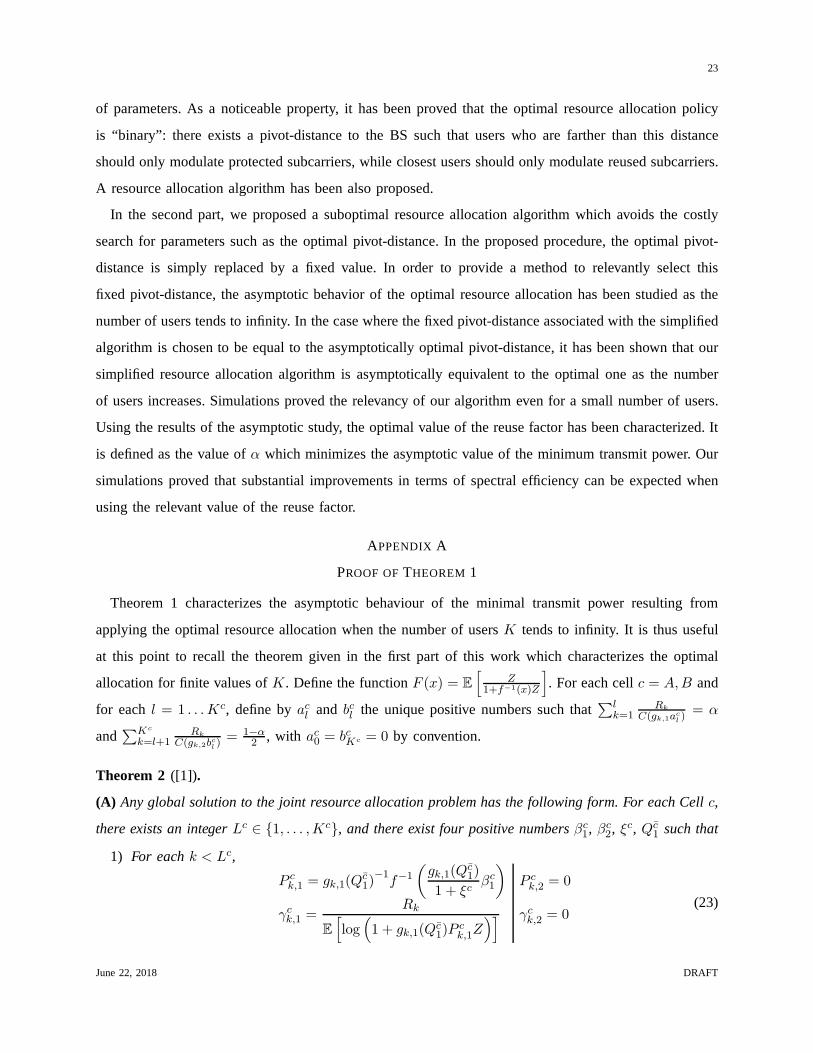
APPENDIX A

PROOF OFTHEOREM 1

Theorem 1 characterizes the asymptotic behaviour of the minimal transmit power resulting from

applying the optimal resource allocation when the number ofusersK tends to infinity. It is thus useful

at this point to recall the theorem given in the first part of this work which characterizes the optimal

allocation for finite values ofK. Define the functionF (x) = E

[

Z1+f−1(x)Z

]

. For each cellc = A,B and

for eachl = 1 . . . Kc, define byacl and bcl the unique positive numbers such that∑l

k=1Rk

C(gk,1acl )

= α

and∑Kc

k=l+1Rk

C(gk,2bcl )

= 1−α2 , with ac0 = bcKc = 0 by convention.

Theorem 2 ([1]).

(A) Any global solution to the joint resource allocation problem has the following form. For each Cellc,

there exists an integerLc ∈ {1, . . . ,Kc}, and there exist four positive numbersβc1, βc2, ξ

c, Qc1 such that

1) For eachk < Lc,

P ck,1 = gk,1(Qc1)

−1f−1

(

gk,1(Qc1)

1 + ξcβc1

)

P ck,2 = 0

γck,1 =Rk

E

[

log(

1 + gk,1(Qc1)P

ck,1Z

)] γck,2 = 0(23)

June 22, 2018 DRAFT

24

2) For eachk > Lc,

P ck,1 = 0 P ck,2 = g−1k,2f

−1(gk,2βc2)

γck,1 = 0 γck,2 =Rk

E

[

log(

1 + gk,2Pck,2Z

)]

(24)

3) For k = Lc

P ck,1 = gk,1(Qc1)

−1f−1

(

gk,1(Qc1)

1 + ξcβ1

)

P ck,2 = g−1k,2f

−1(gk,2βc2)

γck,1 = α−k−1∑

l=1

γcl,1 γck,2 =1− α

2−

Kc

∑

l=k+1

γcl,2.(25)

(B) For eachc = A,B, the systemSc(QA1 , QB1 ) formed by the following four equations is satisfied.

Lc = min

{

l = 1 . . . Kc/gl,1(Q

c1)

1 + ξcF

(

gl,1(Qc1)

1 + ξcal

)

≤ gl,2F (gl,2bl)

}

(26)

gLc,1(Qc1)

1 + ξcF

(

gLc,1(Qc1)

1 + ξcβc1

)

= gLc,2F (gLc,2βc2) (27)

γcLc,1C

(

gLc,1(Qc1)

1 + ξcβc1

)

+ γcLc,2C(gL,2βc2) = RLc (28)

Lc

∑

k

γck,1Pck,1 = Qc1 , (29)

where the values ofγck,1 andP ck,1 in (29) are the functions of(βc1, βc2, ξ

c) defined by equation (23).

(C) Furthermore, for eachc = A,B and for any arbitrary valuesQA1 and QB1 , the system of equations

Sc(QA1 , QB1 ) admits at most one solution(Lc, βc1, β

c2, ξ

c).

In subsection IV-A2, we obtained that for each cellc = A,B,

Qc,(K)1 =

Kc

B

∫∫

∆c,(K)1

rF(x, βc,(K)1 , Q

c,(K)1 , ξc,(K))dνc,(K)(r, x) + oK(1) (30)

Qc,(K)2 =

Kc

B

∫∫

∆c,(K)2

rF(x, βc,(K)2 , 0, 0)dνc,(K)(r, x) + oK(1) (31)

where ∆c,(K)1 = [0, ρ] × [ǫ, dc,(K)] and ∆

c,(K)2 = [0, ρ] × [dc,(K),D] and wheredc,(K) is the pivot-

distancei.e., the position of userLc,(K). Our aim is to prove thatQ(K)T =

∑

cQc,(K)1 +Q

c,(K)2 converges

asK → ∞, and to characterize the limit. For each cellc ∈ {A,B}, sequencedc,(K) is bounded by

definition (dc,(K) ∈ [0,D]). Consider a subsequenceφK such that(dA,(φK), dB,(φK)) converges to a

certain limit, say(dA, dB). We prove that in this case, all quantitiesQc,(φK)1 , Qc,(φK)

2 , βc,(φK)1 , βc,(φK)

2 ,

ξc,(φK) converge to some valuesQc1, Qc2, β

c1, β

c2, ξ

c which we shall characterize. Focus for instance on

sequenceβc,(φK)2 . Recalling thatγc

Lc,(K),2 tends to zero asK → ∞ (γcLc,(K),2 = oK(1)) and replacing

DRAFT June 22, 2018

25

eachγck,2 with expression (23)γck,2 = Rk/C(gck,2βc,(K)2 ), we obtain immediately

1

B

∑

k>Lc,(K)

rkG(x, βc,(K)2 , 0, 0) + oK(1) =

1− α

2, (32)

where we defined

G(x, β,Q, ξ) =1

C(

g1(x,Q)1+ξ β

) (33)

for eachx, β,Q, ξ. In the asymptotic regime, we obtain the following lemma.

Lemma 2. AsK → ∞, sequenceβc,(φK)2 converges to the unique solutionβc2 to the following equation:

t

2

∫ ρ

0

∫ D

dcrG(x, βc2, 0, 0)dν

c(r, x) =1− α

2. (34)

Proof: Existence and uniqueness of the solution to (34) is straightforward since functionβ 7→

G(x, β,Q, ξ) is strictly decreasing from∞ to 0 onR+. We remark that sequenceβc,(φK)2 is boundedi.e.,

βc,(φK)2 ≤ κ for a certain constantκ. In order to prove this claim, assume that there exists a subsequence

βc,φζ(K)

2 which converges to infinity. This hypothesis implies that the subsequence given by the lhs of (32)

for K of the formK = ζ(K ′) converges to zero asK ′ → ∞. This is in contradiction with (32) which

states that the latter sequence converges to1−α2 . Using similar arguments, it can be shown thatβ

c,(φK)2

is lower bounded by a certainǫ′ > 0 i.e., ǫ′ < βc,(φK)2 < κ. Denote byβ2 any accumulation point of

βc,(φK)2 and defineβc,(θK)

2 a subsequence ofβc,(φK)2 (i.e., θK coincides withφζ(K) for a certain function

ζ) which converges toβ2. We prove thatβ2 is given by (34). DefineG(r, x, y) = rG(x, y, 0, 0). We show

that the difference

∆K =

∣

∣

∣

∣

∫ ρ

0

∫ D

dc,(θK )

G(r, x, βc,(θK )2 )dνc,(θK)(r, x) −

∫ ρ

0

∫ D

dcG(r, x, β

c,(θK )2 )dνc(r, x)

∣

∣

∣

∣

tends to zero asK → ∞. By the triangular inequality,

∆K ≤

∣

∣

∣

∣

∫ ρ

0

∫ D

dc,(θK )

G(r, x, βc,(θK )2 )dνc,(θK)(r, x)−

∫ ρ

0

∫ D

dcG(r, x, β

c,(θK )2 )dνc,(θK)(r, x)

∣

∣

∣

∣

+

∣

∣

∣

∣

∫ ρ

0

∫ D

dcG(r, x, β2)dν

c,(θK)(r, x) −

∫ ρ

0

∫ D

dcG(r, x, β

c,(θK )2 )dνc(r, x)

∣

∣

∣

∣

+

∫ ρ

0

∫ D

dc

∣

∣

∣G(r, x, β

c,(θK )2 )−G(r, x, β2)

∣

∣

∣dνc,(θK)(u, x) .

Respectively denote by∆K,1, ∆K,2, ∆K,3 the first, second and third terms of the above equation. We

first study∆K,1. Clearly, functionG(u, x, β) is bounded on[0, ρ] × [ǫ,D] × [ǫ′, κ]. Denote byξ an

upper bound. Then,∆K,1 ≤ ξνθKc (IK), whereIK = [0, ρ] × [dc,(θK), dc] (or IK = [0, ρ]× [dc, dc,(θK)] if

dc < dc,(θK)). Recall thatdc,(θK) converges todc by definition, so thatνc(IK) = ζc([0, ρ])λc([dc,(θK), dc])

June 22, 2018 DRAFT

26

converges to zero as long as measureλc has no mass point atdc. Sinceνc,(θK) converges weakly toνc,

it is straightforward to show thatνc,(θK)(IK), and thus∆K,1, tend to zero. Now focus on∆K,2. The first

term∫ ∫

G(r, x, β2)dνc,(θK)(r, x) which composes∆K,2 converges to

∫ ∫

G(r, x, β2)dνc(r, x) by the

weak convergence ofνc,(θK) to νc. The second term∫ ∫

G(r, x, βc,(θK )2 )dνc(r, x) converges to the same

limit by Lebesgue’s dominated convergence Theorem. Thus,∆K,2 tends to zero. In order to prove that

∆K,3 tends to zero, we remark thatsup∣

∣

∣

∂G(x,r,β)∂β

∣

∣

∣<∞, where the supremum is taken w.r.t.(x, r, β) ∈

[0, ρ]×[ǫ,D]×[ǫ′, κ]. Denote byC the latter supremum. We easily obtain∣

∣

∣G(r, x, β

c,(θK )2 )−G(r, x, β2)

∣

∣

∣≤

C∣

∣

∣βc,(θK)2 − β2

∣

∣

∣, so that∆K,3 ≤ C

∣

∣

∣βc,(θK)2 − β2

∣

∣

∣νθKc ([0, ρ]×[dc,D]). SinceνθKc is a probability measure,

∆K,3 ≤ C∣

∣

∣βc,(θK)2 − β2

∣

∣

∣. Thus∆K,3 tends to zero asK tends to infinity. Putting all pieces together,∆K

tends to zero. Using (32),t2∫ ρ

0

∫ D

dcG(r, x, β

c,(θK )2 )dνc(r, x) converges to1−α2 . By continuity arguments,

β2 = limK βc,(θK)2 satisfies (34). Thusβc,(φK)

2 is a bounded sequence such that any accumulation point

is equal toβ2 defined by (34). ThuslimK βc,(φK)2 = β2.

Using Lemma 2, we may now characterize the limit of (31) asK → ∞. Using the fact that

limK βc,(φK)2 = βc2 and limK d

c,(φK) = dc along with some technical arguments which are similar to the

ones used in the proof of Lemma 2, we obtain

Qc,(φK)2 =

Kc

B

∫ ρ

0

∫ D

dcrF(x, βc2, 0, 0)dν

c,(φK )(r, x) + oK(1) (35)

whereβc2 is the unique solution to (34). Asνc,(φK) converges weakly toνc, Qc,(φK)2 converges to

Qc2 =t

2

∫ ρ

0

∫ D

dcrF(x, β2, 0, 0)dν

c(r, x) . (36)

The same approach can be used to analyze the behavior of sequencesQc,(φK)1 and βc,(φK)

1 for each

c = A,B. After similar derivations, we obtain the following result. As K → ∞, sequence (βA,(φK)1 ,

QA,(φK)1 , ξA,(φK), βB,(φK)

1 , QB,(φK)1 , ξB,(φK)) converges to theuniquesolution(βA1 , Q

A1 , ξ

A, βB1 , QB1 , ξ

B)

to the following system of six equations:

Qc1 =t

2

∫ ρ

0

∫ dc

ǫ

rF(x, βc1, Qc1, ξ

c) dνc(r, x)

t

2

∫ ρ

0

∫ dc

ǫ

rG(x, βc1, Qc1, ξ

c)νc(r, x) = α

g1(dc, Qc1)

1 + ξcF

(

g1(dc, Qc1)

1 + ξcβc1

)

= g2(dc)F (g2(d

c)βc2)

c = A,B , (37)

whereβc2 and dc are the limits ofβc,(φK)2 and dc,(φK) respectively. We discuss now the existence and

the uniqueness of the solution to the above system of equation. For that sake, recall the definition of

functionsF andG given by (12) and (33) respectively. Note thatF(x, β,Q, ξ) = F(x, β1+ξ ,Q, 0), and that

DRAFT June 22, 2018

27

G(x, β,Q, ξ) = G(x, β1+ξ ,Q, 0). Define βc1 = βc

1

1+ξc for c ∈ {A,B}. By applying this new notation, The

first two equations of system (37) give place to the followingsystem of four equations:

Qc1 =t

2

∫ ρ

0

∫ dc

ǫ

rF(x, βc1, Qc1, 0) dν

c(r, x)

t

2

∫ ρ

0

∫ dc

ǫ

rG(x, βc1, Qc1, 0)ν

c(r, x) = α

c = A,B . (38)

The existence and the uniqueness of the solution(βc1, Qc1)c=A,B to the system (38) was thoroughly studied

in [2]. Applying the results of [2] in our context, we conclude that ( βc1

1+ξc , Qc1)c=A,B = (βc1, Q

c1)c=A,B

is unique. We turn now back to the third equation of system (37) to get the following equalityξc =g1(dc,Qc

1)F“

g1(dc,Qc1)

βc1

1+ξc

”

g2(dc)F (g2(dc)βc2)

−1. The latter equation proves the uniqueness ofξc for c = A,B. The uniqueness

of βc1 follows directly from the same equation.

So far, we have proved the uniqueness of the solution to the system (37) of equation. As for the

convergence of sequences (βA,(φK)1 , QA,(φK)

1 , ξA,(φK), βB,(φK)1 , QB,(φK)

1 , ξB,(φK)) to this unique solution,

its proof is omitted here due to the lack of space, but followsthe same ideas as the proof of convergence

of (βA,(φK)2 , QA,(φK)

2 ) and (βB,(φK)2 , QB,(φK)

2 ) provided above.

So far, me managed to prove that for any convergent subsequence (dA,(φK), dB,(φK)) → (dA, dB), the

set of parameters (Qc,(φK)1 , Qc,(φK)

2 , βc,(φK)1 , βc,(φK)

2 , ξc,(φK))c=A,B converges to some valuesQc1, Qc2, β

c1,

βc2, ξc which are completely characterized by the system of equations (34), (36) and (37), as functions

(dA, dB). Using decompositionνc = ζc × λc, the system formed by equations (34), (36) and (37) is

equivalent to the system (19)-(20)-(21)-(22) provided in Theorem 1. At this point, we thus proved that at

least for some subsequencesφK defined as above, the subsequenceQc,(φK)T converges to a limit which

has the form given by Theorem 1. The remaining task is to provethatQ(K)T is a convergent sequence.

First, note thatQ(K)T is a bounded sequence. Indeed,Q

(K)T is defined as the minimum power that can

be transmitted by the network to satisfy the rate requirements. By definition,Q(K)T is thus less than the

power obtained when using the naive solution which consistsin forcing each base station to transmit

only in the protected band (γck,1 is forced to zero for each userk of each cellc). Now it can easily be

shown that whenK → ∞, the power associated with this naive solution converges toa constant. As a

consequence, one can determine an upper-bound onQ(K)T which does not depend onK.

Second, assume for instance thatQT andQ′

T are two accumulation points of sequenceQ(K)T . By

contradiction, assume thatQT < Q′

T . Extract for instance a certain subsequence ofQ(K)T which converges

to QT . Inside this subsequence, one can further extract a subsequence, sayθK , such that

Q(θK)T −→ QT , dc,(θK) −→ dc, ∀c = A,B

June 22, 2018 DRAFT

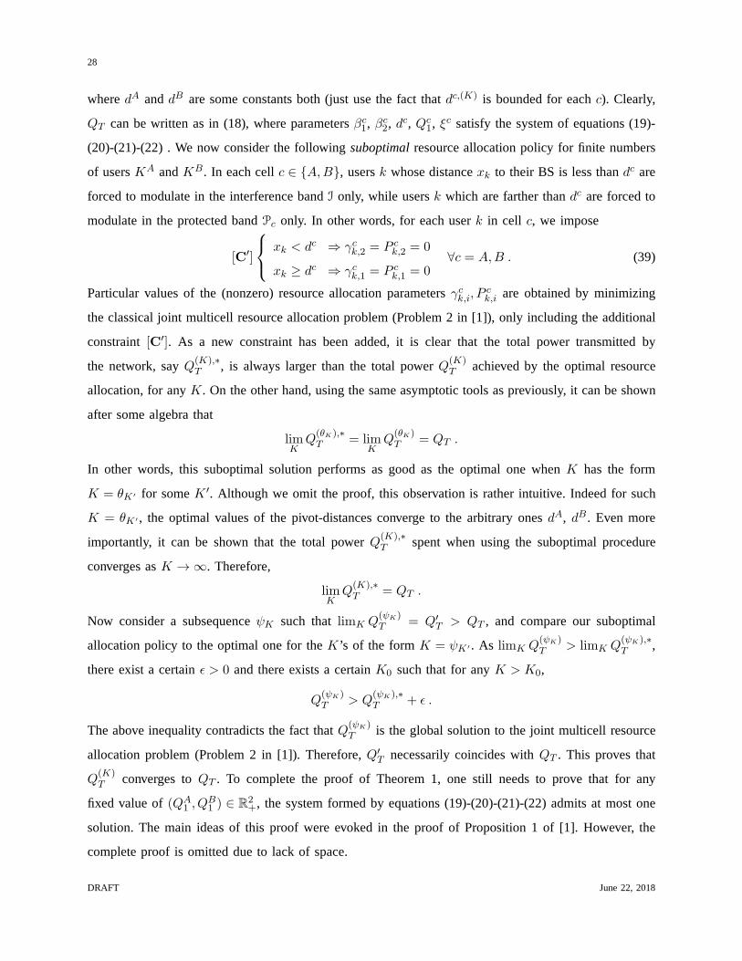
28

wheredA anddB are some constants both (just use the fact thatdc,(K) is bounded for eachc). Clearly,

QT can be written as in (18), where parametersβc1, βc2, d

c, Qc1, ξc satisfy the system of equations (19)-

(20)-(21)-(22) . We now consider the followingsuboptimalresource allocation policy for finite numbers

of usersKA andKB. In each cellc ∈ {A,B}, usersk whose distancexk to their BS is less thandc are

forced to modulate in the interference bandI only, while usersk which are farther thandc are forced to

modulate in the protected bandPc only. In other words, for each userk in cell c, we impose

[C′]

xk < dc ⇒ γck,2 = P ck,2 = 0

xk ≥ dc ⇒ γck,1 = P ck,1 = 0∀c = A,B . (39)

Particular values of the (nonzero) resource allocation parametersγck,i, Pck,i are obtained by minimizing

the classical joint multicell resource allocation problem(Problem 2 in [1]), only including the additional

constraint[C′]. As a new constraint has been added, it is clear that the totalpower transmitted by

the network, sayQ(K),∗T , is always larger than the total powerQ(K)

T achieved by the optimal resource

allocation, for anyK. On the other hand, using the same asymptotic tools as previously, it can be shown

after some algebra that

limKQ

(θK),∗T = lim

KQ

(θK)T = QT .

In other words, this suboptimal solution performs as good asthe optimal one whenK has the form

K = θK ′ for someK ′. Although we omit the proof, this observation is rather intuitive. Indeed for such

K = θK ′ , the optimal values of the pivot-distances converge to the arbitrary onesdA, dB . Even more

importantly, it can be shown that the total powerQ(K),∗T spent when using the suboptimal procedure

converges asK → ∞. Therefore,

limKQ

(K),∗T = QT .

Now consider a subsequenceψK such thatlimK Q(ψK)T = Q′

T > QT , and compare our suboptimal

allocation policy to the optimal one for theK ’s of the formK = ψK ′ . As limK Q(ψK)T > limK Q

(ψK),∗T ,

there exist a certainǫ > 0 and there exists a certainK0 such that for anyK > K0,

Q(ψK)T > Q

(ψK),∗T + ǫ .

The above inequality contradicts the fact thatQ(ψK)T is the global solution to the joint multicell resource

allocation problem (Problem 2 in [1]). Therefore,Q′

T necessarily coincides withQT . This proves that

Q(K)T converges toQT . To complete the proof of Theorem 1, one still needs to prove that for any

fixed value of(QA1 , QB1 ) ∈ R

2+, the system formed by equations (19)-(20)-(21)-(22) admits at most one

solution. The main ideas of this proof were evoked in the proof of Proposition 1 of [1]. However, the

complete proof is omitted due to lack of space.

DRAFT June 22, 2018

29

REFERENCES

[1] N. Ksairi, P. Bianchi, P. Ciblat and W. Hachem,Resource Allocation for Downlink Sectorized Cellular OFDMA Systems:

Part I—Optimal Allocation, 2008.

[2] S. Gault and W. Hachem and P. Ciblat,Performance Analysis of an OFDMA Transmission System in a Multi-Cell

Environment, IEEE Transactions on Communications, num. 12, vol. 55, pp.2143-2159, December, 2005.

[3] J. Chen, R.A. Berry and M. L. Honig,Asymptotic Analysis of Downlink OFDMA Capacity, Forty-Fourth Annual Allerton

Conference, September 2006.

[4] H. Wang and B. Chen,Asymptotic distributions and peak power analysis for uplink OFDMA signals, IEEE International

Conference on Acoustics, Speech, and Signal Processing, May 2004.

[5] E. Biglieri, G. Caire, G. Tarrico and E. Viterbo,How fading affects CDMA: an asymptotic analysis with linearreceivers,

IEEE Journal on Selected Areas in Communications, Volume 19, Issue 2, Pages:191 - 201, February 2001.

[6] D. Gesbert, M. Kountouris,Joint Power Control and User Scheduling in Multi-cell Wireless Networks: Capacity Scaling

Laws,submitted to IEEE Trans. On Information Theory, September 2007.

[7] P. Billingsley , Probability and Measure, 3rd edition Wiley, New York, 1995.

[8] M. Maqbool, M. Coupechoux and Ph. Godlewski,Comparison of Various Frequency Reuse Patterns for WiMAX Networks

with Adaptive Beamforming.IEEE Vehicular Technology Conference, VTC, Singapore, may2008.

[9] H. Jia, Z. Zhang, G. Yu, P. Cheng, and S. Li,On the Performance of IEEE 802.16 OFDMA System under Different

Frequency Reuse and Subcarrier Permutation PatternsProc. of IEEE. ICC, June 2007.

[10] F. Wang, A. Ghosh, C. Sankaran, and S. Benes,WiMAX System Performance with Multiple Transmit and Multiple Receive

Antennas,Proc. of IEEE VTC, April 2007.

[11] T. Thanabalasingham, S. V. Hanly, L. H. Andrew and J. Papandriopoulos, Joint Allocation of Subcarriers and Transmit

Powers in a Multiuser OFDM Cellular Network, IEEE International Conference on Communications ICC ’06,June 2006.

[12] R. D. Yates,A Framework for Uplink Power Control in Cellular Radio Systems, IEEE Journal on Selected Areas in

Communications, vol. 13, no. 7, September 1995.

[13] N. Ksairi, P. Bianchi, P. Ciblat and W. Hachem,Resource Allocation for Downlink Cellular OFDMA Systems: Technical

Report, Tech. Rep., May 2009. Available at http://www.tsi.enst.fr/∼bianchi/Resourceallocation technical report.pdf .

[14] J. F. Bonnans and A. Shapiro,Perturbation analysis of optimization problems,Springer, 2000.

[15] COST Action 231, Digital Mobile Radio toward Future Generation Systems, final report, Tech. Rep., European

Communities, EUR 18957, 1999.

June 22, 2018 DRAFT