1 pros revenue management confidential & proprietary 1 pricing & revenue optimization...

1

PROS Revenue Management Confidential & Proprietary1Pricing & Revenue Optimization

Introducing Information into RM to Introducing Information into RM to Model Market BehaviorModel Market Behavior

INFORMS 6INFORMS 6thth RM and Pricing Conference, Columbia University, NY RM and Pricing Conference, Columbia University, NY

Darius WalczakJune 5, 2006

2 Pricing & Revenue Optimization

OutlineOutline

Introduction Market Priceable demand Introducing Market Information into DP Bellman’s Equation Numerical Examples Conclusions


IntroductionIntroduction

A simple optimization model for a single-resource control problem that includes important elements of competition• A significant portion of demand buys from the seller with lowest

price in the market• We are optimizing from a point of view of one of the competitors• Not a game-theoretic formulation, but…• Inputs to the model can be obtained from such considerations.


Introduction, continuedIntroduction, continued We use the concept of market priceable demand to model behavior of

consumers who seek the lowest price in the market for an otherwise identical product

A seller (controller) captures a portion of that of demand that depends on the state of the market

The state of the market is described by an information variable

We show how to include the information variable in a relatively simple DP formulation of a pricing optimization problem

We present single-resource numerical examples.


Elements of the ModelElements of the Model Introduce a new state variable, market indicator X

• market indicator X is a random variable with known stochastic dynamics

• x, a realization of X, becomes known to the controller before setting price tier for a product

• X can be a null

Introduce a new demand type: Market Priceable Demand

Dynamic Programming formulation with one resource (single-leg) and a product (seat) that can be offered at a finite number of price tiers (price points).


Elements of the Model: ProductElements of the Model: Product

One product offered in the market (easily extendable to a finite number):

The product can be offered at a number of tiers The demand for the product has three components Each competitor has a similar tier structure.


Demand ModelDemand Model

Three components:

• Yieldable demand• Priceable demand• Market Priceable demand

It is assumed that forecasts for each type of demand are available.


Yieldable & Priceable DemandYieldable & Priceable Demand

Yieldable Demand:• Demand at different price points is independent• The product can be offered at different price points simultaneously • Dedicated to tier and seller (requests a specific tier and will not buy

from competition)

Priceable Demand• The demand at the different price points is dependent• Will buy at the lowest price if more than one price point offered at

any given time • Dedicated to seller (will not buy from competition).


Market Priceable DemandMarket Priceable Demand

Market Priceable Demand:

• Demand at different tiers is dependent • Will buy at the lowest tier available in the market• Coin toss if all competitors price the same (same tier offered).


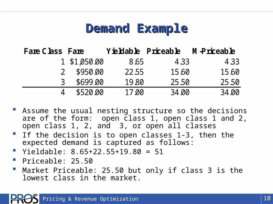
Demand ExampleDemand Example

Assume the usual nesting structure so the decisions are of the form: open class 1, open class 1 and 2, open class 1, 2, and 3, or open all classes

If the decision is to open classes 1-3, then the expected demand is captured as follows:

Yieldable: 8.65+22.55+19.80 = 51 Priceable: 25.50 Market Priceable: 25.50 but only if class 3 is the lowest class in the market.

Fare Class Fare Yieldable Priceable M-Priceable1 $1,050.00 8.65 4.33 4.332 $950.00 22.55 15.60 15.603 $699.00 19.80 25.50 25.504 $520.00 17.00 34.00 34.00


Distributing Market DemandDistributing Market Demand

Rules for distribution of the market priceable demand given each state of the market are assumed known

Consider very simple case with three possible market states:• Noncompetitive (all market priceable demand captured) • Competitive (fair coin-toss, e.g. roughly half captured on average)• Very competitive (completely undercut, nothing captured).


Market DynamicsMarket Dynamics

We consider very simple market dynamics (but it is fairly easy to model a more complex process, time-dependence etc.):

• When a booking request arrives the state of the market (value of the market indicator X) is chosen independently from everything else with given probabilities (e.g. 1/3 for each state, as used later on in the numerical examples).


Bellman’s Equation with Information Bellman’s Equation with Information VariableVariable

Continuous-time formulation with general X

Plus initial and boundary conditions.


Bellman’s Equation, Discrete Time Bellman’s Equation, Discrete Time


Bellman’s Equation, Discrete TimeBellman’s Equation, Discrete Time

The is the probability of the market being in state x

The is the probability of selling a unit of inventory at tier j and in the market state x. This probability is obtained from the three demand components: yieldable, priceable and market priceable

The is the revenue obtained at tier j from all three demand components (an average, since yieldable demand will buy at higher-priced tiers even if tier j has lower price).

xP

xjp ,

jf


Numerical Experiments: ObjectivesNumerical Experiments: Objectives

1. Determine feasibility of running a single-leg DP with the additional state

variable 2. Estimate drop in expected revenue due to not correctly modeling the

market priceable demand in the optimization, i.e. by using an inadequate demand and control model.


Numerical Experiments: MethodologyNumerical Experiments: Methodology

Several scenarios of redistribution of the Market Priceable demand (for the incorrect model) considered:

• The market priceable demand not explicitly modeled but portion of it treated as the yieldable or the priceable demand

• For example, one simple way is to assume that yieldable demand will get 50% of the market priceable demand and the priceable demand will get the same (i.e. both increase due to market priceable demand).


MethodologyMethodology

For each redistribution scenario generate controls (bid prices) from a DP (incorrect model)

Feed them into the DP-based recursion to calculate expected revenues under those controls (with the true market priceable demand present)

Compare the revenues to the revenue under optimal policy with market priceable demand explicitly modeled

Note: This is fully equivalent to running a simulation (Monte Carlo) and comparing revenues under different controls

The advantage is that we do not have any variability issues, disadvantage is that it is only possible in simple settings such as single-leg problems and that we do not model forecasting process.


Numerical Example: Data Numerical Example: Data

Capacity is 136; Fares and Demands:

Market Information Distribution

Fare Class Yieldable Priceable M-Priceable %Priceable %M-Priceable1 ($1050) 8.65 4.33 4.325 25.00% 25.00%2 ($950) 22.55 15.60 15.6 29.02% 29.02%3 ($699) 19.80 25.50 25.5 36.02% 36.02%4 ($520) 17.00 34.00 34 40.00% 40.00%

Market Scenarion Probabilities:NonCompetitive/No Matching 0.333Competitive/Matching 0.334Extremely Competitive/Undercutting 0.333

Portion of Marked Priceable Demand Captured under each scenarion, same for each tier

NonCompetitive/No Matching 1Competitive/Matching 0.5Extremely Competitive/Undercutting 0


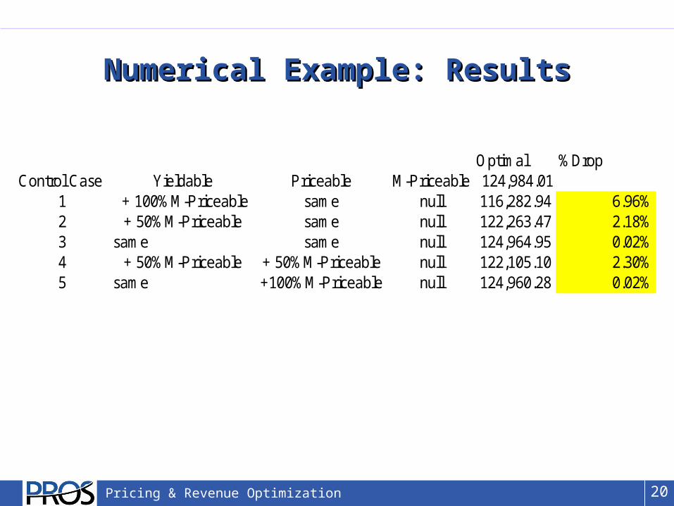
Numerical Example: ResultsNumerical Example: Results

Optimal %DropControl Case Yieldable Priceable M-Priceable 124,984.01

1 + 100%M-Priceable same null 116,282.94 6.96%2 + 50%M-Priceable same null 122,263.47 2.18%3 same same null 124,964.95 0.02%4 + 50%M-Priceable + 50%M-Priceable null 122,105.10 2.30%5 same +100%M-Priceable null 124,960.28 0.02%


Numerical Example: SummaryNumerical Example: Summary Based on this and other similar examples it appears that:

• Revenue decreases as more market priceable demand is modeled as yieldable

• Shifting more of the market priceable to the priceable demand improves performance (smaller decrease)

• Best results when 100% of market priceable modeled as priceable

• Magnitude of differences is very data dependent


ConclusionsConclusions

The run time increase is proportional to the number of states of the information variable (worst case)

Modeling market priceable as priceable demand appears to be better than splitting market priceable

Caveat: we assume forecasts are given

Need to try more complex random dynamics for X


Future ResearchFuture Research

Apply models in competitive simulations• Multiple carriers with their own RM Systems (RMS) competing for the same

demand• Initial results show significant positive revenue lifts• Solution more robust to different data conditions and other carriers’ RMS


ReferencesReferences

Talluri, K. T., G. J. van Ryzin (2004), The Theory and Practice of Revenue Management, Kluwer Academic Publishers.

Walczak, D., “Semi-Markov Information Model for Revenue Management and Dynamic Pricing,” OR Spectrum (Springer), special issue on RM and Pricing, 2006.

25

PROS Revenue Management Confidential & Proprietary25Pricing & Revenue Optimization

Introducing Information into RM to Introducing Information into RM to Model Market BehaviorModel Market Behavior

INFORMS 6INFORMS 6thth RM and Pricing Conference, Columbia University, NY RM and Pricing Conference, Columbia University, NY

Darius WalczakJune 5, 2006

1 pros revenue management confidential & proprietary 1 pricing & revenue optimization...

Documents

type of demand

market information

pricing optimization

new demand type

model market behavior

lowest price

simple optimization

pricing conference