1

Program Correctness

CIS 375

Bruce R. Maxim

UM-Dearborn

2

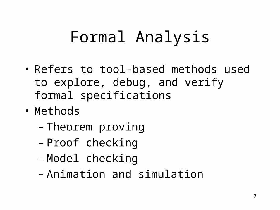
Formal Analysis

• Refers to tool-based methods used to explore, debug, and verify formal specifications

• Methods– Theorem proving– Proof checking– Model checking– Animation and simulation

3

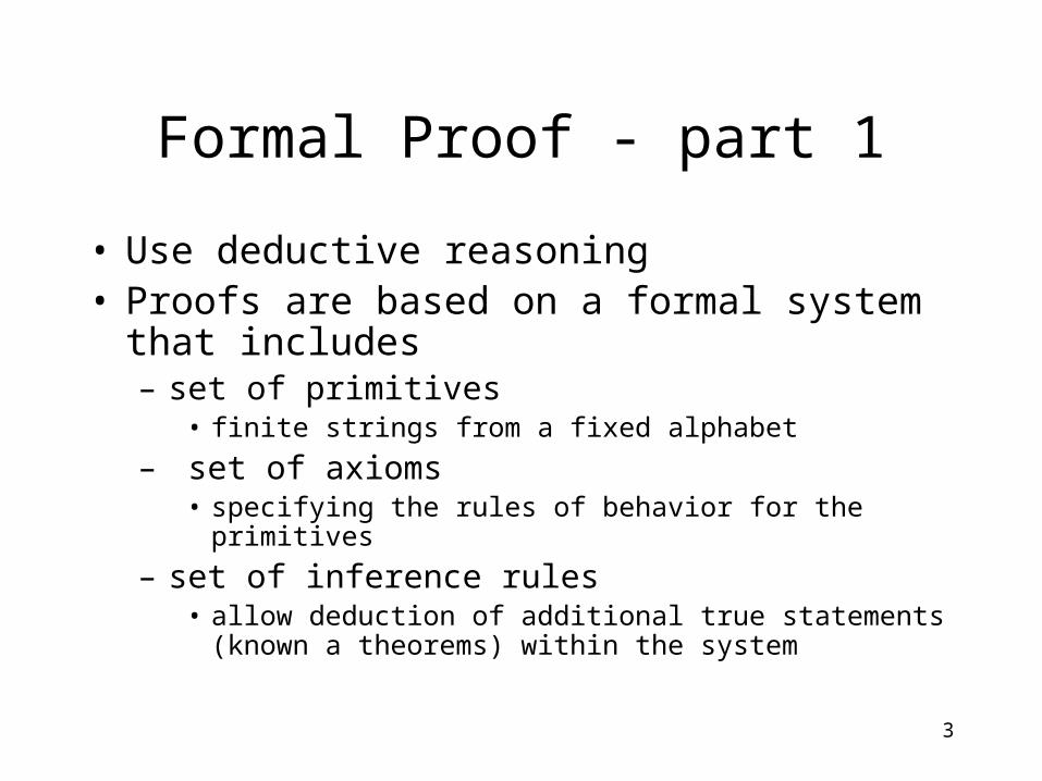
Formal Proof - part 1

• Use deductive reasoning• Proofs are based on a formal system that

includes– set of primitives

• finite strings from a fixed alphabet

– set of axioms• specifying the rules of behavior for the primitives

– set of inference rules• allow deduction of additional true statements (known a

theorems) within the system

4

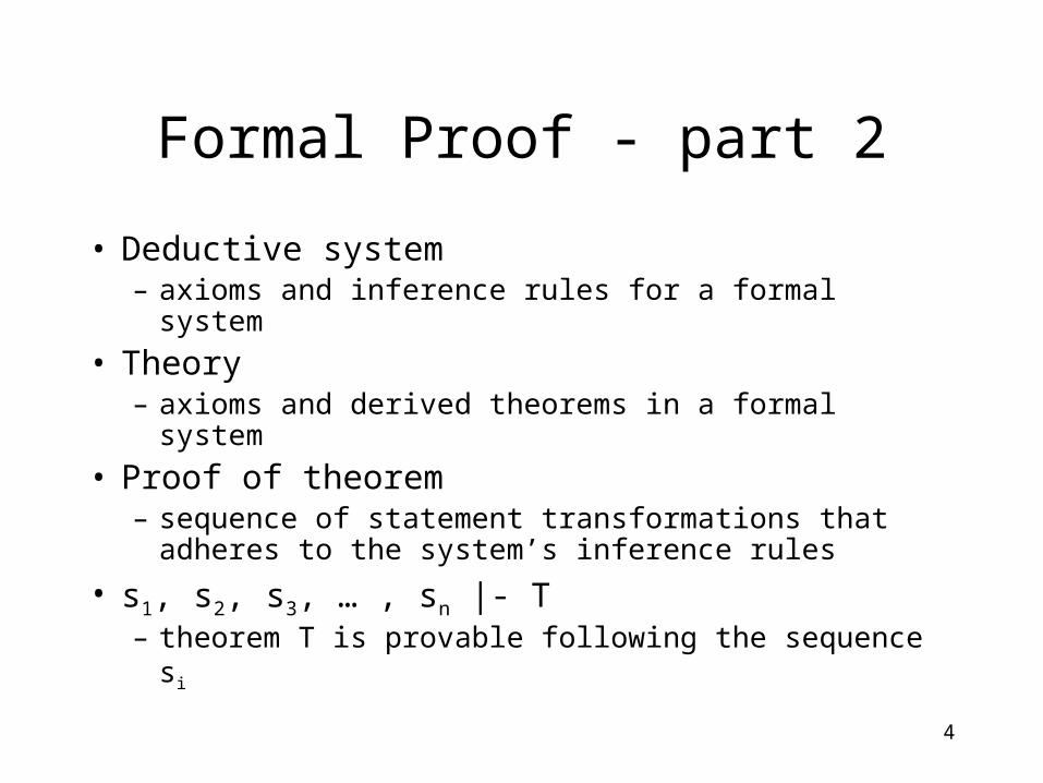
Formal Proof - part 2

• Deductive system– axioms and inference rules for a formal system

• Theory– axioms and derived theorems in a formal system

• Proof of theorem– sequence of statement transformations that

adheres to the system’s inference rules

• s1, s2, s3, … , sn |- T– theorem T is provable following the sequence si

5

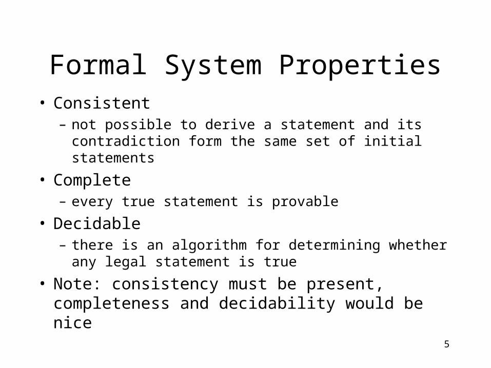
Formal System Properties• Consistent

– not possible to derive a statement and its contradiction form the same set of initial statements

• Complete– every true statement is provable

• Decidable– there is an algorithm for determining whether any

legal statement is true

• Note: consistency must be present, completeness and decidability would be nice

6

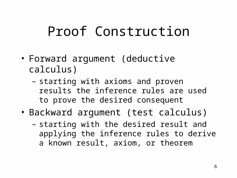
Proof Construction

• Forward argument (deductive calculus)– starting with axioms and proven results the

inference rules are used to prove the desired consequent

• Backward argument (test calculus)– starting with the desired result and applying the

inference rules to derive a known result, axiom, or theorem

7

Mechanical Theorem Provers

• Many mechanical theorem provers require human interaction

• Users typically are required to choose the rule of inference to be applied at each step

• The theorem prover may be able to discover (by heuristic search) some rules to apply on its own

• The user needs to translate the statements to some normal form prior to beginning

8

Program Verification

• Similar to writing a mathematical proof

• You must present a valid argument that is believable to the reader

• The argument must demonstrate using evidence that the algorithm is correct

• Algorithm is correct if code correctly transforms initial state to final state

9

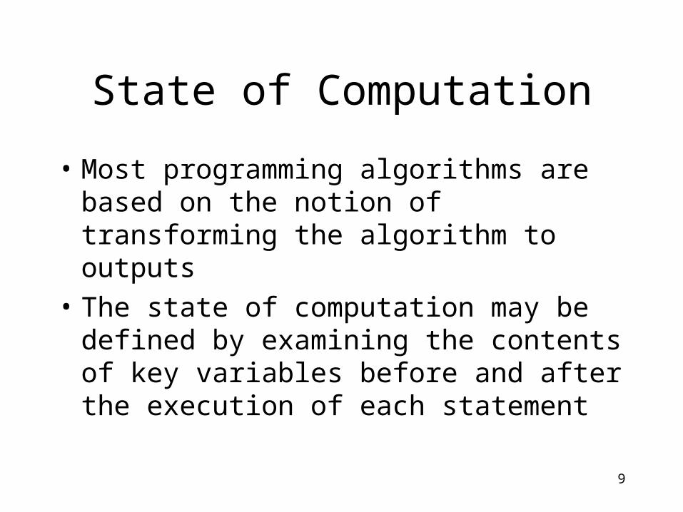
State of Computation

• Most programming algorithms are based on the notion of transforming the algorithm to outputs

• The state of computation may be defined by examining the contents of key variables before and after the execution of each statement

10

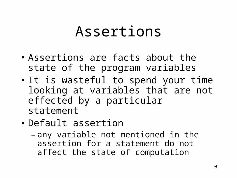
Assertions

• Assertions are facts about the state of the program variables

• It is wasteful to spend your time looking at variables that are not effected by a particular statement

• Default assertion– any variable not mentioned in the assertion

for a statement do not affect the state of computation

11

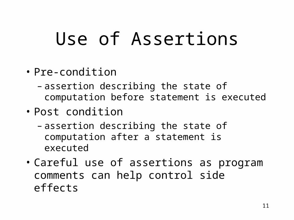
Use of Assertions

• Pre-condition– assertion describing the state of

computation before statement is executed

• Post condition– assertion describing the state of

computation after a statement is executed

• Careful use of assertions as program comments can help control side effects

12

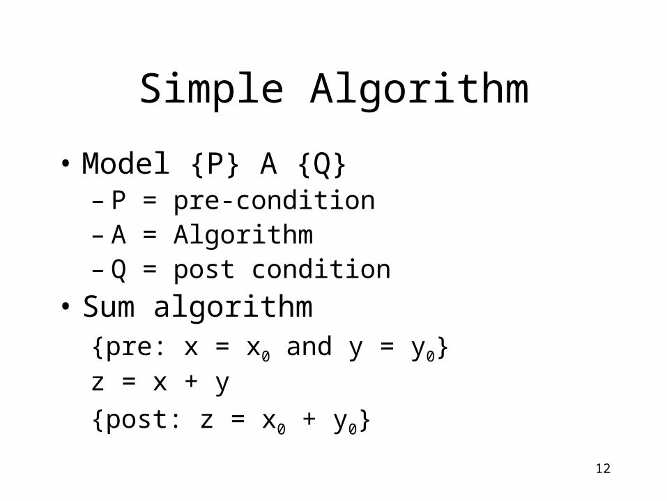
Simple Algorithm

• Model {P} A {Q}– P = pre-condition– A = Algorithm– Q = post condition

• Sum algorithm{pre: x = x0 and y = y0}z = x + y

{post: z = x0 + y0}

13

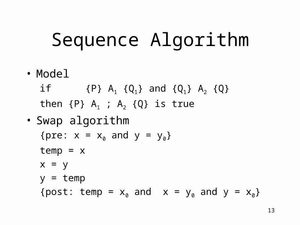
Sequence Algorithm

• Model if {P} A1 {Q1} and {Q1} A2 {Q}

then {P} A1 ; A2 {Q} is true

• Swap algorithm{pre: x = x0 and y = y0}

temp = x

x = y

y = temp

{post: temp = x0 and x = y0 and y = x0}

14

Intermediate Assertions

• Swap algorithm{pre: x = x0 and y = y0}temp = x

{temp = x0 and x = x0 and y = y0}x = y

{temp = x0 and x = y0 and y = y0}y = temp

{post: temp = x0 and x = y0 and y = x0}

15

Conditional Statements

• Absolute value{pre: x = x0}

if x < 0 then

y = - x0

else

y = x0

{post: y = | x0 |}

16

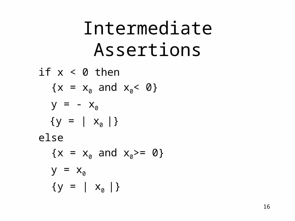
Intermediate Assertions

if x < 0 then

{x = x0 and x0< 0}

y = - x0

{y = | x0 |}

else

{x = x0 and x0>= 0}

y = x0

{y = | x0 |}

17

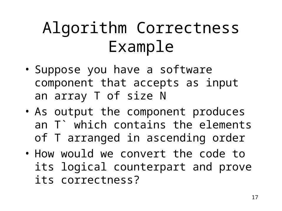
Algorithm Correctness Example

• Suppose you have a software component that accepts as input an array T of size N

• As output the component produces an T` which contains the elements of T arranged in ascending order

• How would we convert the code to its logical counterpart and prove its correctness?

18

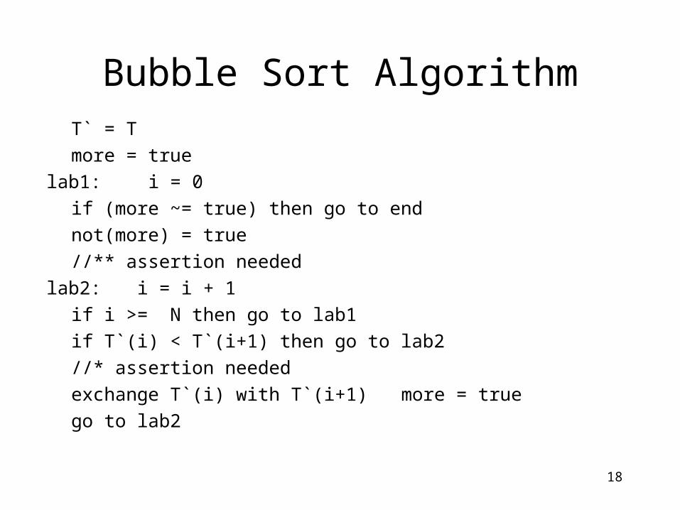
Bubble Sort AlgorithmT` = T

more = true

lab1: i = 0

if (more ~= true) then go to end

not(more) = true

//** assertion needed

lab2: i = i + 1

if i >= N then go to lab1

if T`(i) < T`(i+1) then go to lab2

//* assertion needed

exchange T`(i) with T`(i+1) more = true

go to lab2

19

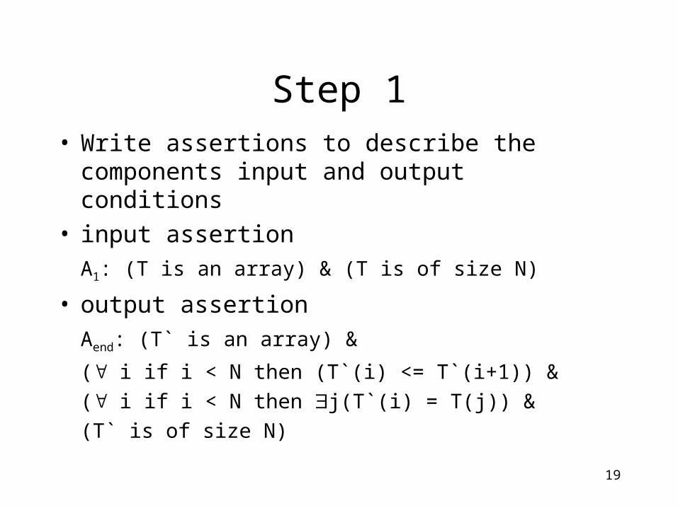
Step 1• Write assertions to describe the components

input and output conditions• input assertion

A1: (T is an array) & (T is of size N)

• output assertion

Aend: (T` is an array) &

( i if i < N then (T`(i) <= T`(i+1)) &

( i if i < N then j(T`(i) = T(j)) &

(T` is of size N)

20

Step 3

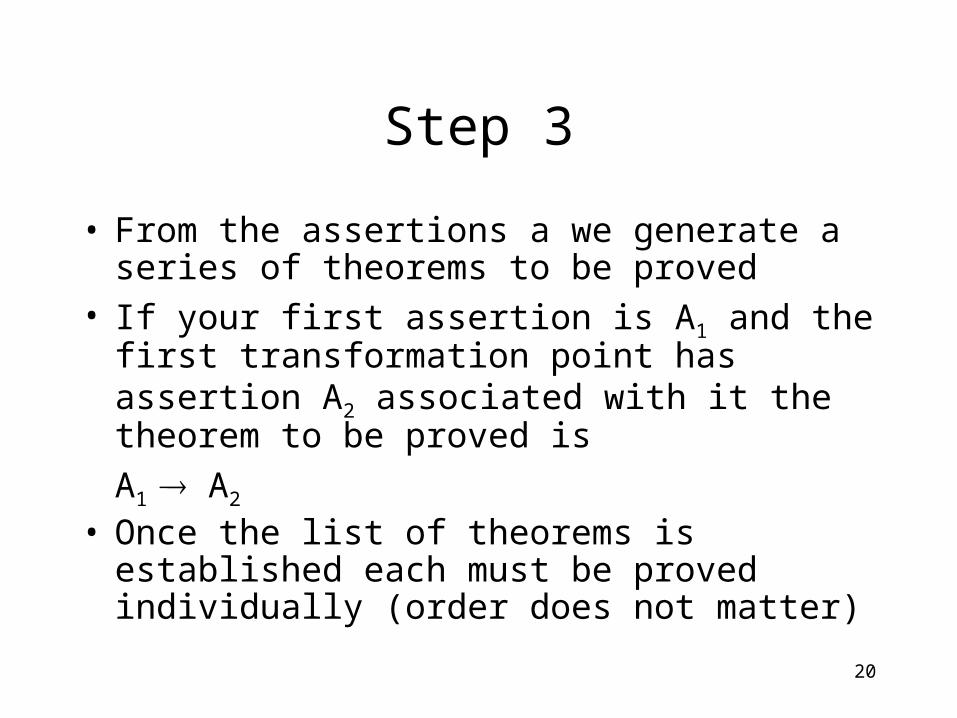
• From the assertions a we generate a series of theorems to be proved

• If your first assertion is A1 and the first transformation point has assertion A2 associated with it the theorem to be proved is

A1 A2

• Once the list of theorems is established each must be proved individually (order does not matter)

21

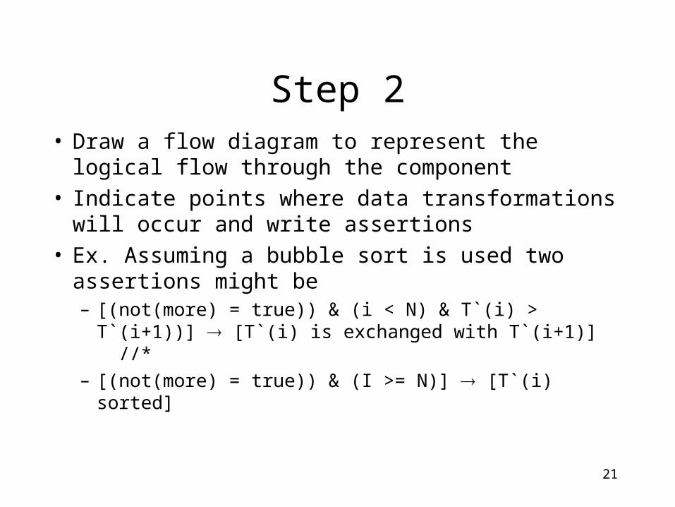
Step 2• Draw a flow diagram to represent the logical

flow through the component • Indicate points where data transformations will

occur and write assertions• Ex. Assuming a bubble sort is used two

assertions might be– [(not(more) = true)) & (i < N) & T`(i) > T`(i+1))]

[T`(i) is exchanged with T`(i+1)] //*– [(not(more) = true)) & (I >= N)] [T`(i) sorted]

22

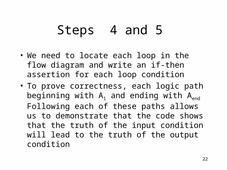
Steps 4 and 5

• We need to locate each loop in the flow diagram and write an if-then assertion for each loop condition

• To prove correctness, each logic path beginning with A1 and ending with Aend Following each of these paths allows us to demonstrate that the code shows that the truth of the input condition will lead to the truth of the output condition

23

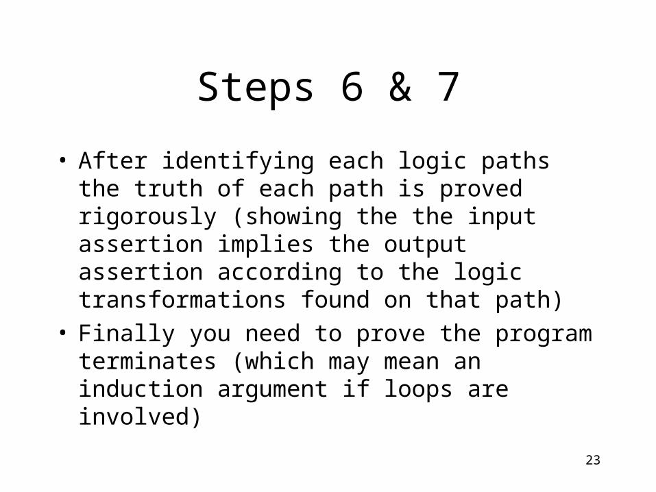
Steps 6 & 7

• After identifying each logic paths the truth of each path is proved rigorously (showing the the input assertion implies the output assertion according to the logic transformations found on that path)

• Finally you need to prove the program terminates (which may mean an induction argument if loops are involved)

24

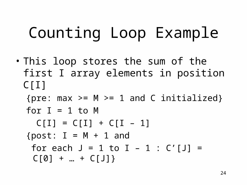
Counting Loop Example

• This loop stores the sum of the first I array elements in position C[I]{pre: max >= M >= 1 and C initialized}

for I = 1 to M

C[I] = C[I] + C[I – 1]

{post: I = M + 1 and

for each J = 1 to I – 1 : C’[J] = C[0] + … + C[J]}

25

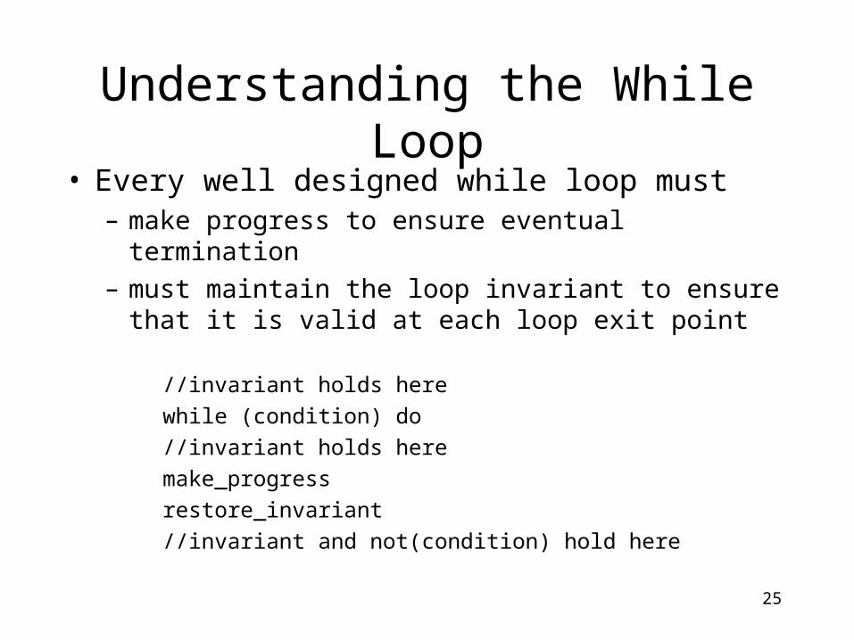
Understanding the While Loop• Every well designed while loop must

– make progress to ensure eventual termination– must maintain the loop invariant to ensure that it is

valid at each loop exit point

//invariant holds here

while (condition) do

//invariant holds here

make_progress

restore_invariant

//invariant and not(condition) hold here

26

Loop Invariant

• Type of assertion that describes the variables which remain unchanged during the execution of a loop

• In general the stopping condition should remain unchanged during the execution of the loop

• Some people show the loop invariant as a statement which becomes false when loop execution is complete

27

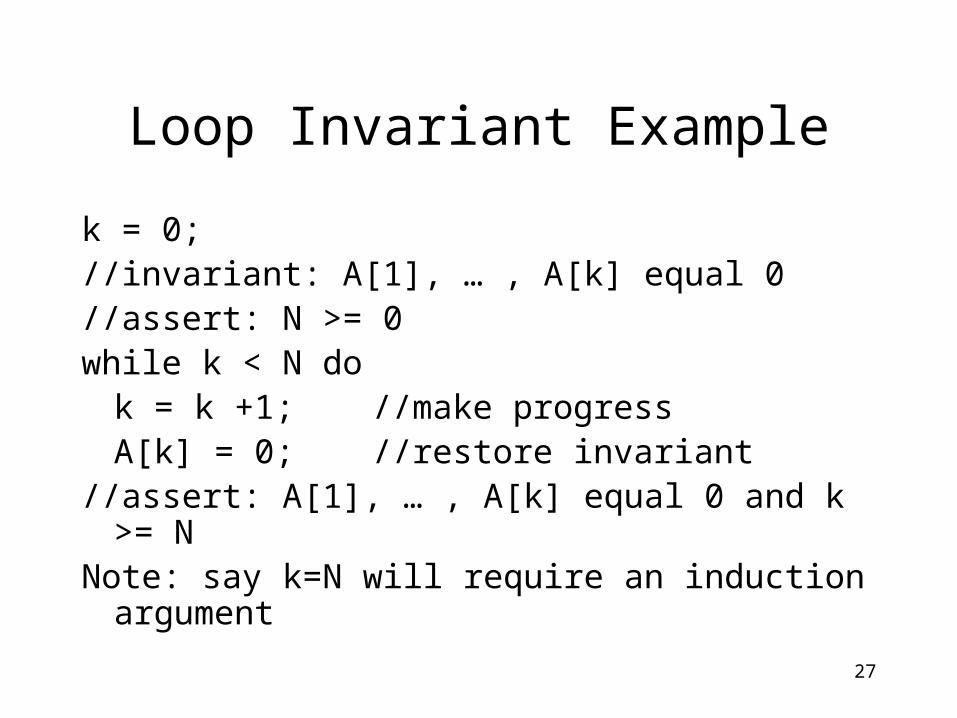
Loop Invariant Example

k = 0;//invariant: A[1], … , A[k] equal 0//assert: N >= 0while k < N do

k = k +1; //make progressA[k] = 0; //restore invariant

//assert: A[1], … , A[k] equal 0 and k >= N Note: say k=N will require an induction

argument

28

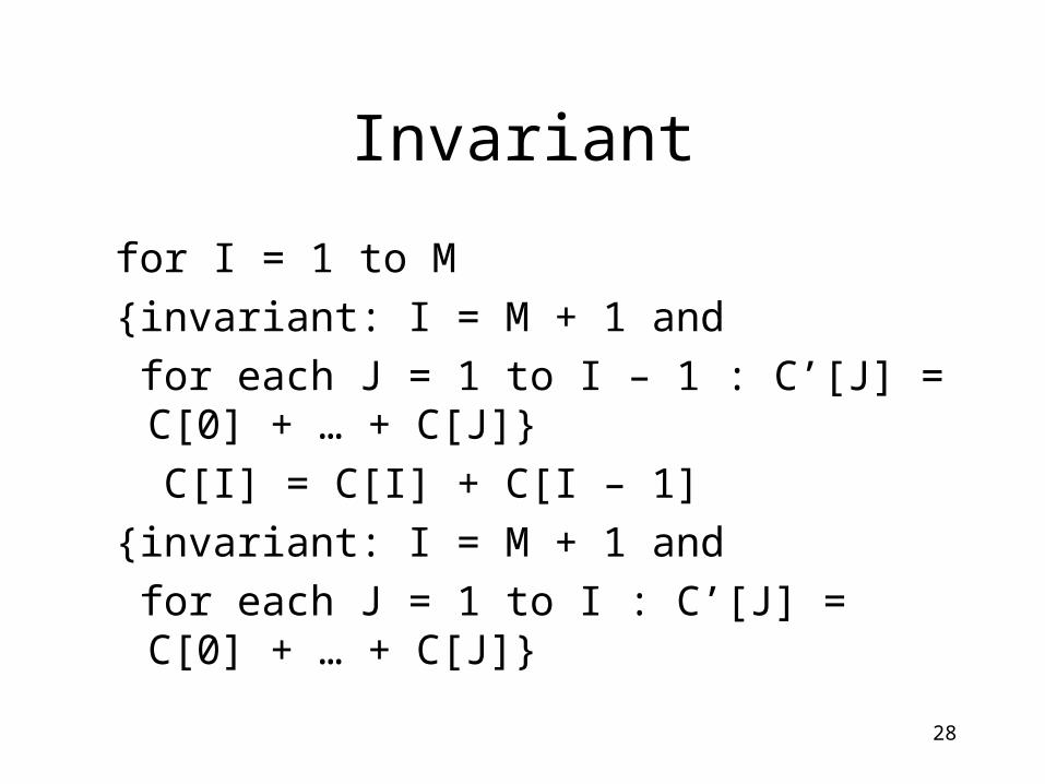
Invariant

for I = 1 to M

{invariant: I = M + 1 and

for each J = 1 to I – 1 : C’[J] = C[0] + … + C[J]}

C[I] = C[I] + C[I – 1]

{invariant: I = M + 1 and

for each J = 1 to I : C’[J] = C[0] + … + C[J]}

29

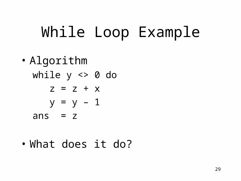
While Loop Example

• Algorithmwhile y <> 0 do

z = z + x

y = y – 1

ans = z

• What does it do?

30

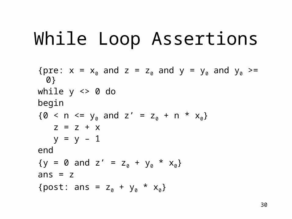
While Loop Assertions

{pre: x = x0 and z = z0 and y = y0 and y0 >= 0}while y <> 0 dobegin

{0 < n <= y0 and z’ = z0 + n * x0} z = z + x y = y – 1end

{y = 0 and z’ = z0 + y0 * x0}ans = z

{post: ans = z0 + y0 * x0}

31

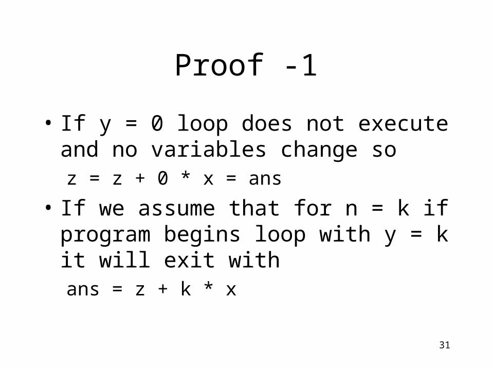
Proof -1

• If y = 0 loop does not execute and no variables change soz = z + 0 * x = ans

• If we assume that for n = k if program begins loop with y = k it will exit withans = z + k * x

32

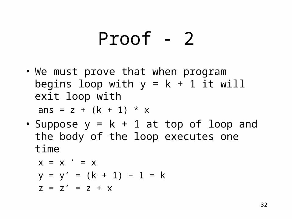
Proof - 2

• We must prove that when program begins loop with y = k + 1 it will exit loop withans = z + (k + 1) * x

• Suppose y = k + 1 at top of loop and the body of the loop executes one timex = x ‘ = x

y = y’ = (k + 1) – 1 = k

z = z’ = z + x

33

Proof - 3

• Since we are at the top of the loop with y = k, we can use our induction hypothesis to getans = z’ + k * x’

• Substituting we getans = (z + x) + k * x

= z + (x + k * x)

= z + (1 + k) * x

= z + (k + 1) * x

34

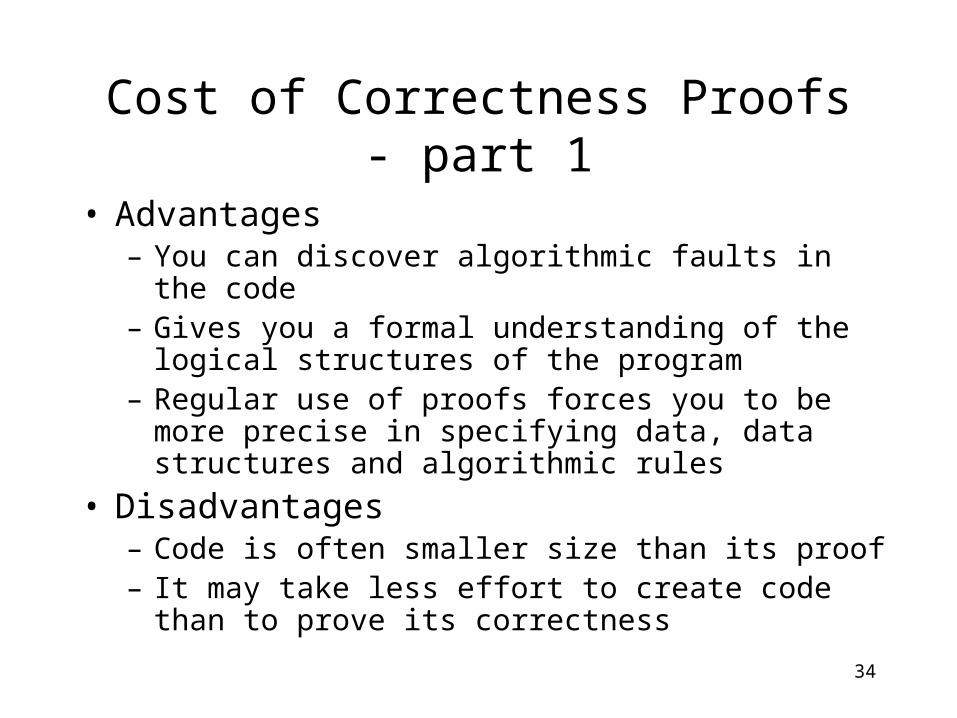
Cost of Correctness Proofs - part 1

• Advantages– You can discover algorithmic faults in the code– Gives you a formal understanding of the logical

structures of the program– Regular use of proofs forces you to be more precise

in specifying data, data structures and algorithmic rules

• Disadvantages– Code is often smaller size than its proof– It may take less effort to create code than to prove

its correctness

35

Cost of Correctness Proofs - part 2

• Disadvantages (continued)– Large programs require complex diagrams and

contain many transformations to prove– Nonnumeric algorithms are hard to represent

logically– Parallel processing is hard to represent– Complex data structures require complex

transformations– Mathematical proofs have occasionally been found

to be incorrect after years of use

36

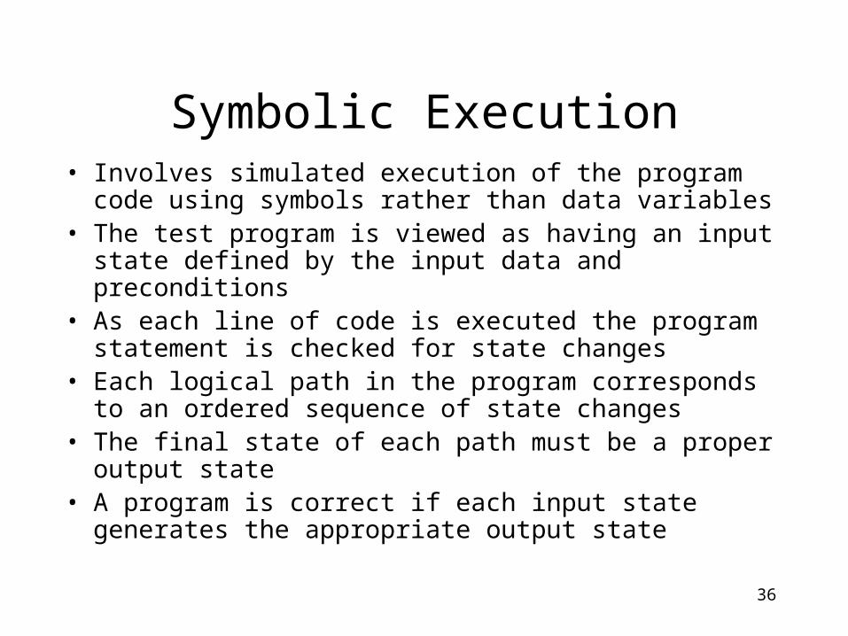
Symbolic Execution• Involves simulated execution of the program code

using symbols rather than data variables• The test program is viewed as having an input state

defined by the input data and preconditions• As each line of code is executed the program

statement is checked for state changes• Each logical path in the program corresponds to an

ordered sequence of state changes• The final state of each path must be a proper output

state• A program is correct if each input state generates the

appropriate output state

37

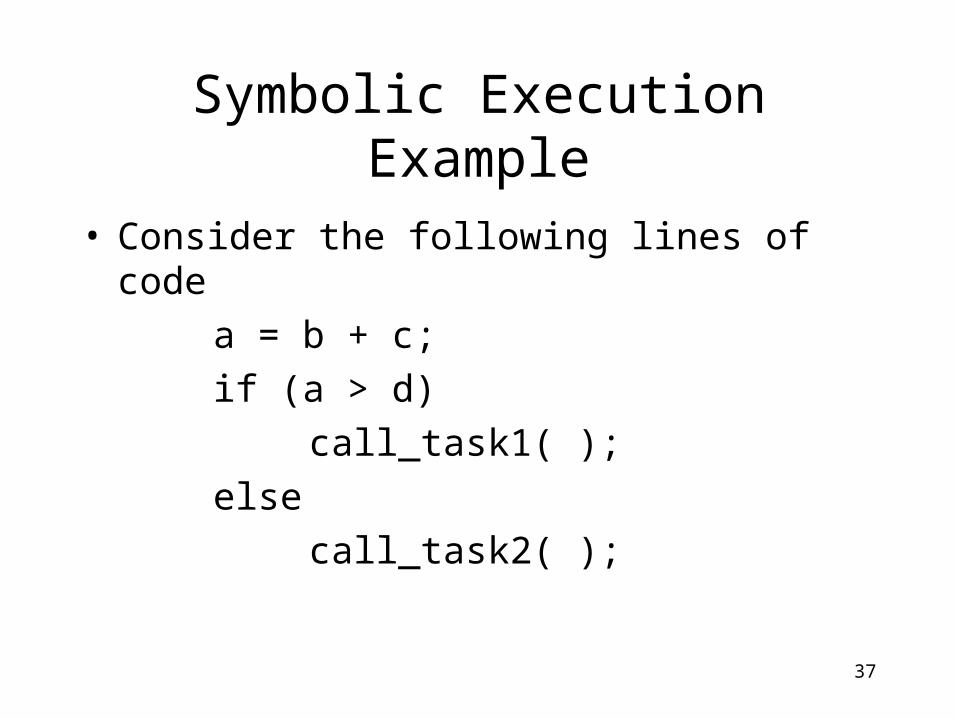
Symbolic Execution Example

• Consider the following lines of code

a = b + c;

if (a > d)

call_task1( );

else

call_task2( );

38

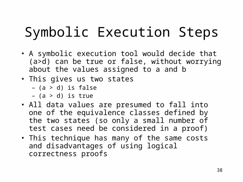
Symbolic Execution Steps

• A symbolic execution tool would decide that (a>d) can be true or false, without worrying about the values assigned to a and b

• This gives us two states– (a > d) is false– (a > d) is true

• All data values are presumed to fall into one of the equivalence classes defined by the two states (so only a small number of test cases need be considered in a proof)

• This technique has many of the same costs and disadvantages of using logical correctness proofs

39

Structural Induction

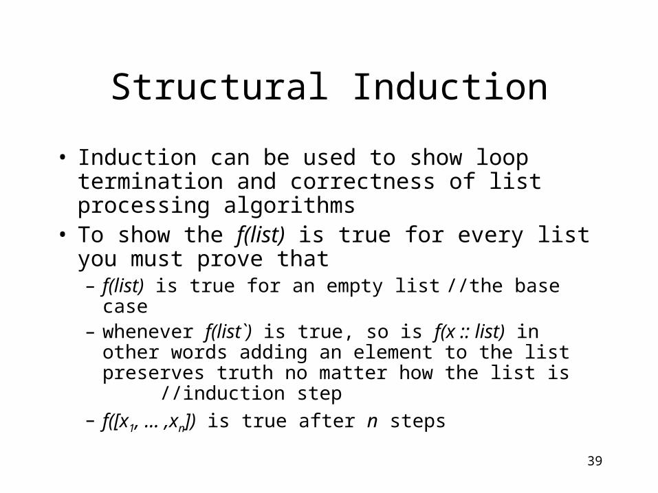
• Induction can be used to show loop termination and correctness of list processing algorithms

• To show the f(list) is true for every list you must prove that– f(list) is true for an empty list //the base case– whenever f(list`) is true, so is f(x :: list) in other

words adding an element to the list preserves truth no matter how the list is //induction step

– f([x1, … ,xn]) is true after n steps

40

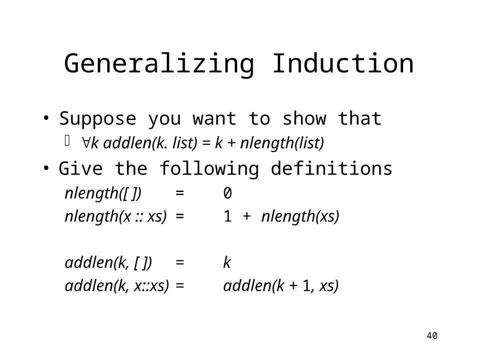
Generalizing Induction

• Suppose you want to show that k addlen(k. list) = k + nlength(list)

• Give the following definitionsnlength([ ]) = 0

nlength(x :: xs) = 1 + nlength(xs)

addlen(k, [ ]) = k

addlen(k, x::xs) = addlen(k + 1, xs)

41

Induction Correctness Proof

k addlen(k. list) = k + nlength(list)• Base case:

addlen(k, [ ]) = k

= k + 0

= k + nlength([ ])

• Induction step - assume that

addlen(k, x::list`) = addlen(k + 1, list`)

= k + 1 + nlength(list`) //IHOP

= k + nlength(x :: list`) // must prove