1

Preferences and Utility

(Chapters 3, 4)

2

1. Preferences 1a. A single consumption good

Consider a world with a single consumption good. A corresponding consumption bundle would list the amount of that single good, (x1).

If the good is really a “good” (rather than a bad or a neutral), we know how any individual would feel about two different bundles: the bundle with more of the good would be strictly preferred. We could also define weak preference and indifference. All the notions of preference would depend on concepts of equality and inequality of real numbers.

weak preference: ≥ , the usual “greater than or equal to”

strict preference: >, the usual “strictly greater than”

indifference: =, the usual “equal to”

3

1b. Two consumption goods

Consider a world with two consumption goods. A corresponding consumption bundle would least the amount of each good, (x1, x2).

If both goods are really “goods” (rather than bads), then if one bundle had more of each of the goods, it would be strictly preferred by any individual. However, if one bundle had more of the first good but less of the second good than the second bundle, then different individuals might rank the two bundles differently. As an analog to the equality and inequality concepts for numbers, we introduce preference concepts for bundles of two (or more) goods.

4

weak preference, “at least as good as” or “weakly preferred to”

strict preference, “preferred to” is derived from weak preference: (x1, x2) is strictly preferred to (y1, y2) if it is weakly preferred to (y1, y2), and (y1, y2) is not weakly preferred to it.

indifference is derived from weak preference: (x1, x2) is indifferent to (y1, y2) if it is weakly preferred to (y1, y2), and (y1, y2) is weakly preferred to it.

Maintained assumption: Unless stated otherwise, we will assume that each of the two goods may be consumed in any nonnegative amount (i.e., quantities need not to be integers).

5

2. Economic Assumptions about Preferences*

Compare the following assumptions to what you know about inequalities and numbers.

2a. Rationality assumption: weak preferences are complete and transitive

complete means any two bundles can be ranked

transitive means the ranking has no cycles (i.e., it is not possible to find three bundles such that the first is strictly better than the second, which is strictly better than the third, which is strictly better than the first)

The Rationality Assumption implies strict preference and indifference are also transitive. However they are not complete (why?).

6

2b. Continuity assumption:

if we consider a sequence of bundles, each of which is as good as (x1, x2), the limit of the sequence must also be as good as (x1, x2). Similarly, if the bundles in the sequence are no better than (x1, x2) then the limit is no better than (x1, x2).

2c. Monotonicity or nonsatiation assumption

version 1: if (x1, x2) has more of each good than (y1, y2), then it is strictly preferred

version 2: if (x1, x2) has more of one good and no less of other good than (y1, y2), then it is strictly preferred.

7

3. Indifference Curves

An indifference curve is a set of bundles all of which are indifferent to each other.

An indifference curve is a “level curve” in the sense that all bundles on the curve have the same level of preference. There is a different indifference curve for each different level of preference.

With the assumptions from section 2, distinct indifference curves cannot intersect and movement to northeast leads to preferred indifference curves

8

4. Utility Functions

Utility functions allow us to examine consumer behavior using calculus rather than set theory. A utility function is a function that assigns numbers to consumption bundles.

A utility function u represents preferences u(x1, x2)≥u(y1, y2) if and only if (x1, x2) is weakly preferred to (y1, y2).

If the rationality and continuity assumptions hold, then there exists a utility function representing preferences.

If there is a utility function representing preferences, it is not unique.

The number assigned matters only in an ordinal sense. This means all that matters is whether one’s bundle is higher than that of another bundle. The actual numbers assigned can be positive or negative, large or small.

With a utility function, indifference curves are just level curves of the utility function.

9

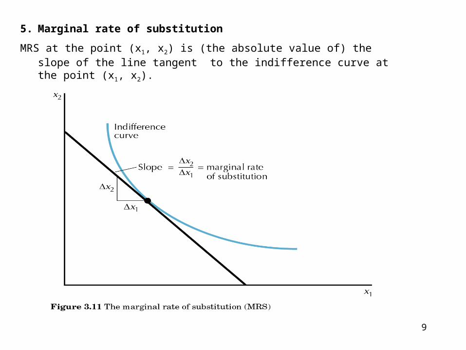
5. Marginal rate of substitution

MRS at the point (x1, x2) is (the absolute value of) the slope of the line tangent to the indifference curve at the point (x1, x2).

10

If there is a differentiable utility function, then MRS is the ratio of marginal utilities

MRS=U1 (x1, x2)/U2 (x1, x2)

where U1 (x1, x2) is the partial derivative of the utility function with respect to the first good and U2 (x1, x2) is the partial derivative of the utility function with respect to the second good.

Generally MRS depends on the point (x1, x2).

11

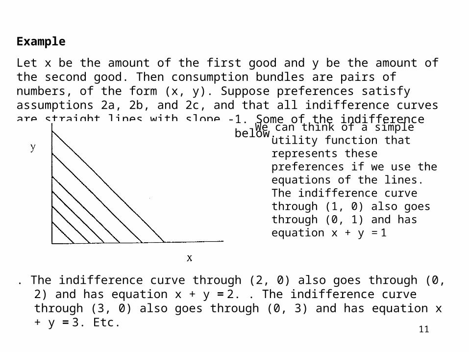
Example

Let x be the amount of the first good and y be the amount of the second good. Then consumption bundles are pairs of numbers, of the form (x, y). Suppose preferences satisfy assumptions 2a, 2b, and 2c, and that all indifference curves are straight lines with slope -1. Some of the indifference curves are shown in the figure below.

We can think of a simple utility function that represents these preferences if we use the equations of the lines. The indifference curve through (1, 0) also goes through (0, 1) and has equation x + y = 1

. The indifference curve through (2, 0) also goes through (0, 2) and has equation x + y = 2. . The indifference curve through (3, 0) also goes through (0, 3) and has equation x + y = 3. Etc.

12

Consider as a possible utility function

u(x, y) = x + y.

Does this satisfy the requirements? Yes. Comparing two bundles of goods, it assigns a higher number to the bundle on the “better” indifference curve.

This is not the only utility function that represents these preferences. As alternatives we could use

u*(x, y) = x + y - 103

(note the fact that u* is sometimes negative is irrelevant) or

u**(x, y) = (x + y)2.

Note at any point (x, y), the MRS is 1. (The indifference curves all have slope – 1, and the ratio of marginal utilities is 1.)

13

7. Important special classes of preferences

We will consider several important classes of preferences. Each class is made up of many different preferences that have some important common feature. (We will also use these same classes when we discuss production later.)

The previous example can be generalized to a special class of preferences, generalized perfect substitutes.

14

7a. The class of (generalized) perfect substitutes

For any member of this class of preferences, all indifference curves are parallel, straight lines.

The preferences can be represented by a utility function of the form

u(x, y)=ax + by

where “a” and “b” are positive numbers such that –a/b is equal to the slope of the indifference curves.

Note that the marginal rate of substitution is constant: MRS = a/b at every point (x, y).

Examples:

For an individual who thinks “all colas are the same,” if the goods are liter bottles of Coke and liter bottles of Pepsi, then the MRS is always 1.

For most individuals, if the goods are $5 bills and $10 bills, then the MRS is always 1/2.

15

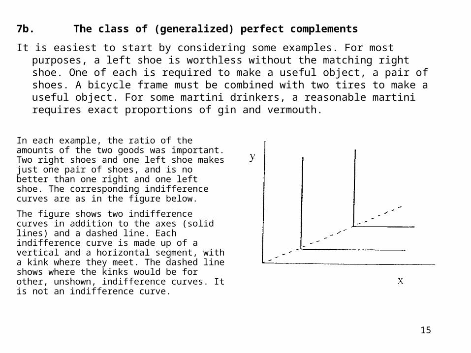
In each example, the ratio of the amounts of the two goods was important. Two right shoes and one left shoe makes just one pair of shoes, and is no better than one right and one left shoe. The corresponding indifference curves are as in the figure below.

The figure shows two indifference curves in addition to the axes (solid lines) and a dashed line. Each indifference curve is made up of a vertical and a horizontal segment, with a kink where they meet. The dashed line shows where the kinks would be for other, unshown, indifference curves. It is not an indifference curve.

7b.The class of (generalized) perfect complements

It is easiest to start by considering some examples. For most purposes, a left shoe is worthless without the matching right shoe. One of each is required to make a useful object, a pair of shoes. A bicycle frame must be combined with two tires to make a useful object. For some martini drinkers, a reasonable martini requires exact proportions of gin and vermouth.

16

The preferences can be represented by a utility function of the form

u(x, y) = minimum {x/a, y/b}

where “a” and “b” are positive numbers and “minimum” means take the smaller of the two numbers (e.g., the smaller of the number of left shoes and the number of right shoes determines the number of usable pairs of shoes). The ratio a/b is determined by the slope of the dashed line in the figure since the point (x, y) = (a, b) lies on that line (x/a = a/a = 1 = b/b = y/b).

Note that the marginal rate of substitution is undefined at the kink and 0 (on

the horizontal segment) or “∞” (on the vertical segment) elsewhere.

17

7c. The classes of parallel preferences (or quasi-linear utility)

(There are two related classes, one corresponding to vertical shifts and the other to horizontal shifts.)

For these preferences, all indifference curves look the same, and are formed by taking one indifference curve and shifting it (vertically for one class, horizontally for the other). An example of the vertical shift case is given in the figure.

The preferences are said to be parallel.

These preferences can be represented by (quasi-linear) utility functions of the form

u(x, y) = f(x) + y (for the vertical shift case)

or

u(x, y) = x + g(y) (for the horizontal shift case)

The utility function is said to be quasi-linear because in each case one of the goods appears as a linear term while the other appears as the argument in an increasing function.

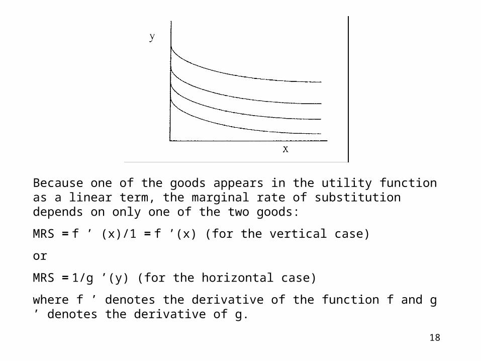
18

Because one of the goods appears in the utility function as a linear term, the marginal rate of substitution depends on only one of the two goods:

MRS = f ’ (x)/1 = f ’(x) (for the vertical case)

or

MRS = 1/g ’(y) (for the horizontal case)

where f ’ denotes the derivative of the function f and g ’ denotes the derivative of g.

19

7d.The Cobb-Douglas class of preferences

This is a handy subclass of the class of homothetic preferences. For homothetic preferences, the marginal rate of substitution is constant along any ray through (0, 0), but it may be different along different rays. Thus the MRS is a function of the ratio, x/ y.

The Cobb-Douglas class consists of those homothetic preferences that can be represented by utility functions of the form

u(x, y) = xayb

where “a” and “b” are positive numbers. Another utility function representing the same preferences (and sometimes easier to work with) is

u*(x, y) = a*ln(x) + b*ln(y)

where “a” and “b” are the same positive numbers and ln( ) is the natural logarithm function.

Using u*, the partial derivatives pf the utility function are a/x with respect to x and b/y with respect to y, so the marginal rate of substitution is

MRS = ay/bx = (alb)(y/x), which is a function of the ratio of x to y.

20

8. Convexity of preferences

A final property of preferences that will be useful to us has to do with the shape of indifference curves.

Consider any single indifference curve and any two bundles of goods, say bundle A and bundle B, each of which is weakly preferred to bundles on the indifference curve. If it is always the case that all the bundles on the line segment joining bundle A and bundle B are also weakly preferred to bundles on the indifference curve, then the preferences are called weakly convex. If it is always the case that all the bundles on the line segment joining bundle A and bundle B are strictly preferred to bundles on the indifference curve, then the preferences are called strictly convex.

21

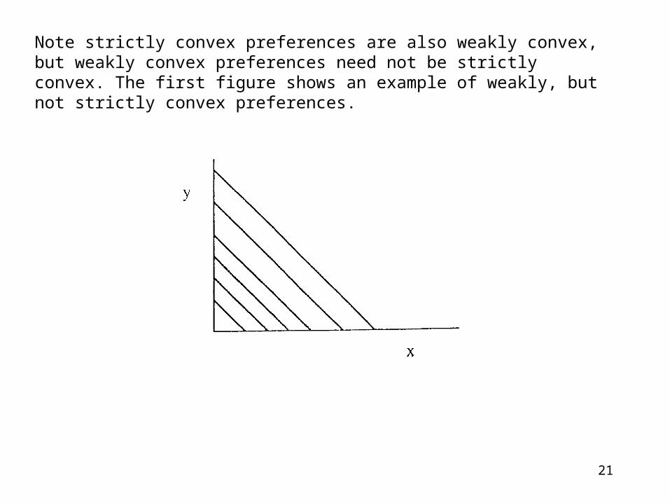
Note strictly convex preferences are also weakly convex, but weakly convex preferences need not be strictly convex. The first figure shows an example of weakly, but not strictly convex preferences.

22

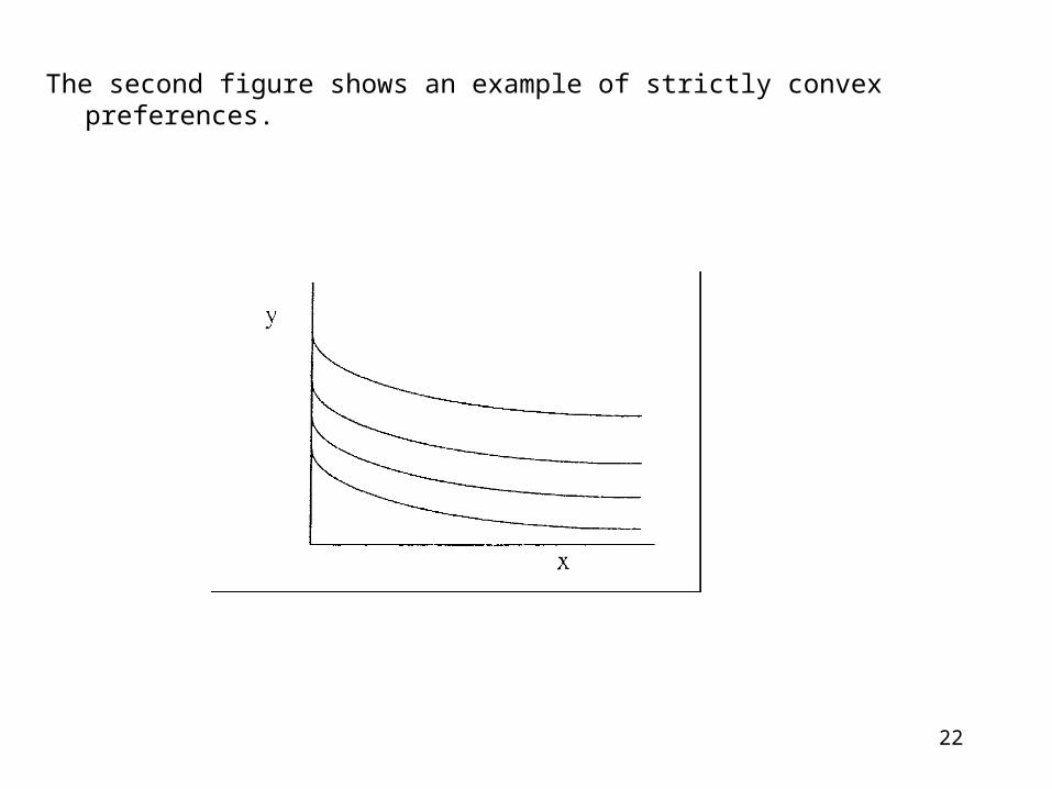
The second figure shows an example of strictly convex preferences.

23

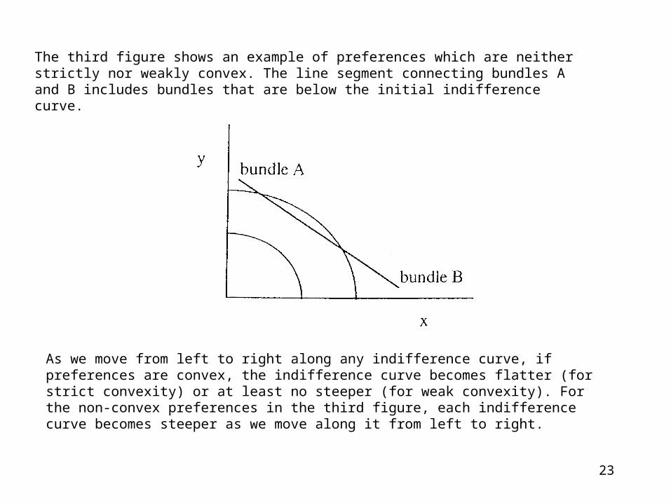
The third figure shows an example of preferences which are neither strictly nor weakly convex. The line segment connecting bundles A and B includes bundles that are below the initial indifference curve.

As we move from left to right along any indifference curve, if preferences are convex, the indifference curve becomes flatter (for strict convexity) or at least no steeper (for weak convexity). For the non-convex preferences in the third figure, each indifference curve becomes steeper as we move along it from left to right.

24

These are general results. Since the marginal rate of substitution is just the absolute value of the slope of the indifference curve, for convex preferences, the MRS (at least weakly) diminishes as we move from left to right along any indifference curve.

We will be using convex preferences (diminishing MRS). Of the classes of preferences introduced in Section 7, perfect substitutes (7a) and perfect complements (7b) are weakly convex while Cobb-Douglas (7d) are strictly convex [except when considering two bundles of the form (x, 0) or two bundles of the form (0, y)].

25

For the quasi-linear utility classes (7c), additional assumptions are needed. For the vertical shift case, with utility function

u(x,y)=f(x)+y

the preferences are weakly convex if the second derivative of f is non-positive and strictly convex if the second derivative of f is strictly negative. For the horizontal case, with

u(x, y) =x + g(y)

similar conditions hold for the function g.