1

Part III

FPGA Design FPGA Design SoftwareSoftware

2

IntroductionIntroduction

Two-level synthesis

Multi-level synthesis

PLA(1980)

Symbolic minimization

FunctionalDecompositio

n(1995)

Technology development?

1984 (Espresso)

3

Basic Structures of programmable devices

PLA

P Lrogrammable ogic rrayA

FPGA

F P G Aield rogrammable ate rray

GA, SC

G A

S C

ate rray

tandard ell

4

Simple Computer Aided Design System

Synteza logicznai

odwzorowanie technologiczne

S ymu la to r

Prog ra m ato r

Specyfikacjaprojektu

KOMPILACJA

Weryfikacjai programowanie

Edytorgraficzny

Edytortekstowy

Wykresyczasowe

Analizatoropóźnień

abcdeabcdeabcde

S ta nd a rd CAES ta n d ard CAE

Project specification

compilation

Logic Synthesis and Technology Mapping

Verification and Programming

Graphic Editor

Text Editor

Timing Editor

Timing Analyzer

Simulator

Programmer

PLA/PLD Logic PLA/PLD Logic OptimizationOptimization

7a

PLA, PLDFPGA

Reduction

Silicon Area(# CLBs)

6

PLA

x

x

x

1

2

n

f

f

f

0

1

- 1m

1 2 p

AND

OR

7

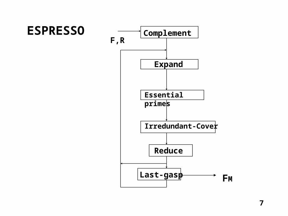
ESPRESSO ComplementF,R

FM

Expand

Essential primes

Irredundant-Cover

Reduce

Last-gasp

8

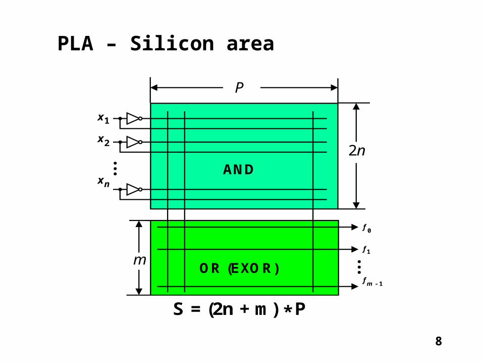
PLA – Silicon area

x

x

x

1

2

n

f

f

f

0

1

- 1m

AND

OR (EXOR)

P

2n

m

S = (2n + m) * P

9

Example – adder realisation

X1

X2

X3

X4

f

f

f

1

2

3

X1

X3

X2

X4

f

f

f

1

2

3

Two-input decoder

10

Types of PLA structures

A N D

O R

A N D

E X O R

A N D

O R

A N D

E X O R

AND-OR z dekoderem

1-bitowym

AND-EXOR z dekoderem

1-bitowym

AND-OR z dekoderem

2-bitowym

AND-EXOR z dekoderem

2-bitowym

AND-OR with one-bit decoder

AND-EXOR with one-bit decoder

AND-OR with two-bit decoder

AND-EXOR with two-bit decoder

11

PLA with two-bit decoder

x + x1 2

x + x1 2

x + x1 2

x + x1 2

x

x

1

2

x

x

n

n

- 1

p p p 1 j t

y

y

y

1

i

m

12

Two Level PLA(Ciesielski)

P L A n

I n

P L A 1

I 1

P L A 2

I 2P L A 2

I

f

P L A

I

f

MinimalizacjasymbolicznaSymbolic Minimization

13

Symbolic minimization

ADDR OPC CNTR

INDEX AND CNTA

INDEX OR CNTA

INDEX JMP CNTA

INDEX ADD CNTA

DIR AND CNTB

DIR OR CNTB

DIR JMP CNTC

DIR ADD CNTC

IND AND CNTB

IND OR CNTD

IND JMP CNTD

IND ADD CNTC

DEKODER

OPC

ADDR

CNTRDecoder

14

Symbolic Minimization

ADDR OPC CNTR

100 1000 1000 ADDR OPC CNTR

100 0100 1000 100 1111 1000 100 0001 1000 010 1100 0100 100 0010 1000 001 1000 0100 010 1000 0100 001 0101 0001 010 0100 0100 010 0011 0010 010 0001 0010 001 0010 0010

010 0010 0010 001 1000 0100 001 0100 0001 001 0001 0001 001 0010 0010

Encoded Table Table after Espresso Minimization

15

Two bit adder

C a a b bi 1 0 1 0

C y yi + 1 1 0

S u m a t o r

e b a d c

f f f0 1 2

F

wejścia/wyjścia oznaczenia w tablicy prawdyInputs/outputs

Adder

Notation in the truth table

Next page cont

16

Symbolic Minimization

a b c d e f0 f1 f2– 1 0 0 0 0 1 00 1 – 0 0 0 1 0– 0 0 1 0 0 1 00 0 – 1 0 0 1 01 0 – 0 1 0 1 00 0 0 1 – 0 1 0– 0 1 0 1 0 1 00 1 0 0 – 0 1 01 0 1 0 – 0 1 01 – 0 – 0 1 0 00 – 1 – 0 1 0 00 – 0 – 1 1 0 0– 1 1 1 1 0 1 01 1 – 1 1 0 1 01 1 1 1 – 0 1 01 – 1 – 1 1 0 0– – 1 1 1 0 0 11 – –1 1 0 0 1– 1 1 – 1 0 0 11 1 – – 1 0 0 11 – 1 1 – 0 0 11 1 1 – –– 1 – 1 –

0 0 10 0 1

a

b

c

d

e

f

f

f

0

1

2

Sumatordwubitowy

e d c+ b af f f2 1 0

Positional Notation

a c e 0 0 0 (first)

– 0 0 1 0 0 0 1 0 0 0

1 0 0 (fifth)

Two-bit adder

17

Adder Realization using symbolic minimizationX1 = (a,c,e) X2 =(b,d)

01234567 0123 f0 f1 f2

10001000 0010 0 1 0

10100000 0010 0 1 0

10001000 0100 0 1 0

10100000 0100 0 1 0

00000101 1000 0 1 0

11000000 0100 0 1 0

00010001 1000 0 1 0

11000000 0010 0 1 0

00000011 1000 0 1 0

00001000 1111 1 0 0

00100000 1111 1 0 0

01000000 1111 1 0 0

00010001 0001 0 1 0

00000101 0001 0 1 0

00000011 0001 0 1 0

00000001 1111 1 0 0

00010001 0202 0 0 1

00000101 0101 0 0 1

00010001 0011 0 0 1

00000101 0011 0 0 1

00000011 0101 0 0 1

00000011 0011 0 0 1

11111111 0001 0 0 1

X1 = (a,c,e) X2 =(b,d)

11101000 0110 010

00010111 1001 010

00010111 0110 001

01101001 1111 100

11111111 0001 001

18

Two-bit adder Realization

f

f

f

0

1

2

P L A 1 2

P L A 2

P L A 1 1

a

c

e

b

d

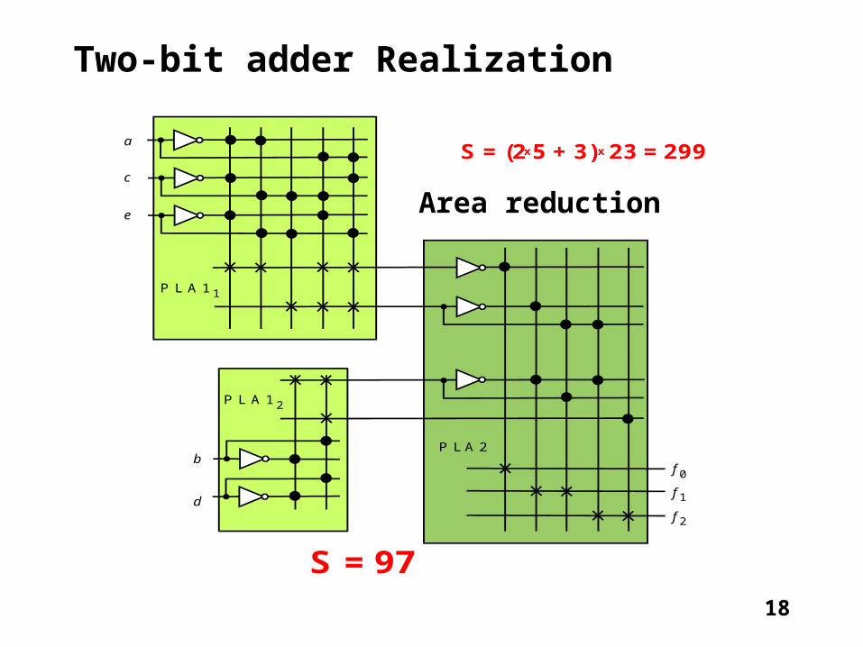
S = (2 5 + 3) 23 = 299x x

Redukcja powierzchni !

S = 97

Area reduction

19

Sequential Circuits based on PLA/PLD

D

ANDI S ORS' O

IN OUT

IN PS NS OUT

Minimalizacjawielowratościowa

Kodowanie stanów

PLA z minimalną powierzchnią

symbolic minimization = Minimization of the number ofStates of encoding

21a

Multi-valued minimization

State Encoding

PLA with minimal area

20

FLEX 10K with Embedded Array Blocks

LogicArray

I/O Element(IOE)

Logic Element(LE)

Logic Array Block(LA B)

EmbeddedAr rayBlock

EmbeddedArrayBlock

Fast TrackInterconnect

IOE IOE IOE IOE IOE IOE

IOE IOE IOE IOE IOE IOE

IOE

IOE

IOE

IOE

IOE

IOE

IOE

IOE

ROM

21

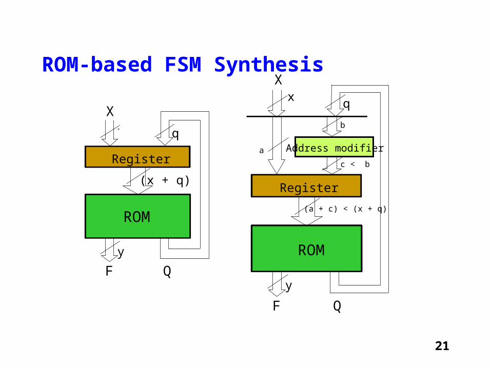
ROM-based FSM SynthesisX

F Q

ROM

Register

Address modifier

qx

a

b

c < b

(a + c) < (x + q)

y

X

F Q

ROM

Register

qx

(x + q)

y

22

FPGAFPGA based Logic based Logic SynthesisSynthesis

K om ó rkalog iczn a

I /O

Ka na łypo łąc ze niow echannels

CLBs

23

Logic Synthesis

• Logic minimization.

• Technology dependent/independent minimization.

• Technology mapping.

24

Physical Synthesis

• Placement.

• Routing.

25

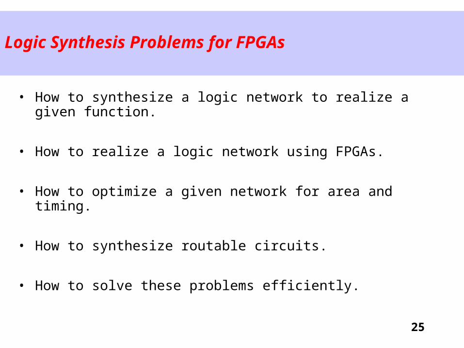
Logic Synthesis Problems for FPGAs

• How to synthesize a logic network to realize a given function.

• How to realize a logic network using FPGAs.

• How to optimize a given network for area and timing.

• How to synthesize routable circuits.

• How to solve these problems efficiently.

26

Representation of Boolean Functions

• Truth tables.• Factored forms: SOP and POS.• BDD.• Boolean networks.

27

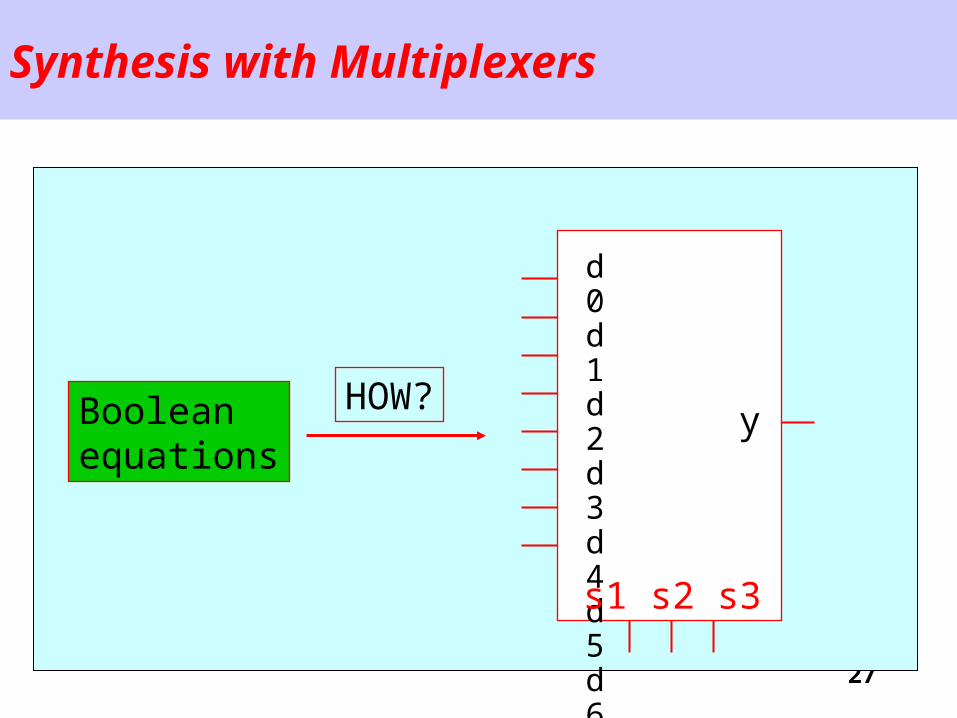
Synthesis with Multiplexers

d0d1d2d3d4d5d6d7

s1 s2 s3

yBooleanequations

HOW?

28

Synthesis with Look-Up-Table (LUT)

d0d1d2d3d4d5d6d7

yBooleanequations

HOW?LUT

29

An Example of synthesis of the same function with various components

XOR(a,b) = a’b + ab’

d0d1d2d3

s0 s1

y

01

MUX

0

0

1

1

Dec

odera

b

RAM

30

Multilevel Logic Minimization

• MIS and SIS by UC Berkeley.

• Optimization for timing, area, and power.

• Technology independent.

31

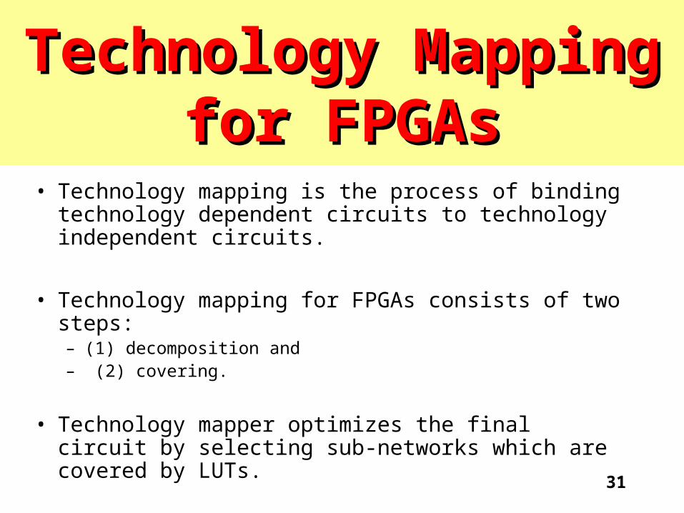
Technology Mapping Technology Mapping for FPGAsfor FPGAs

• Technology mapping is the process of binding technology dependent circuits to technology independent circuits.

• Technology mapping for FPGAs consists of two steps: – (1) decomposition and– (2) covering.

• Technology mapper optimizes the final circuit by selecting sub-networks which are covered by LUTs.

32

Technology Mapping for FPGAs

• LUTs have fixed number of inputs, k-input, which can implement logic functions up to k variables.

• Nodes and sub-networks with at most k inputs in a Boolean network are referred to feasible nodes and sub-networks else infeasible.

• Infeasible nodes need to be decomposed into a set of feasible nodes so that a circuit covering the network exists.

33

Technology Mapping for FPGAs

An FPGA-based technology mapper performs three tasks:

1. Decomposition - It decomposes infeasible expressions into feasible ones.

2. Reduction - It groups small expressions into CLBs to promote sharing of resources.

3. Packing - It allocates CLBs to expressions that cannot be shared.

34

Technology Mapping for FPGAs

• The optimization goals for FPGA-based technology mapping include:

1. The number of CLBs,

2. The number of levels of CLB circuits, and

3. Routable designs.

35

DeDeccompoompositionsition

abcabdacdbcd

ff

a

b

c

d

f = abc + abd + acd + bcd f = gh + gh

g = abh = c + d

Realizacja funkcji f

przed dekompozycją po dekompozycjiBefore decomposition

After decomposition

Realization of a function:

36

Decomposition

– Decomposition consists of three steps:

• Identify divisors which are common to

many functions.

• Introduce the divisor as a new node.

• Re-express existing nodes using the new nodes.

37

An Example

• Given the expression

f = ab’+ac’+ad’+a’b+bc’+bd’+a’c+b’c+cd’+b’d+c’d

• Suppose a factor found is p = a+b+c+d

• f can be re-expressed based on p: f = p(a’+b’+c’+d’)

38

Shannon Cofactoring

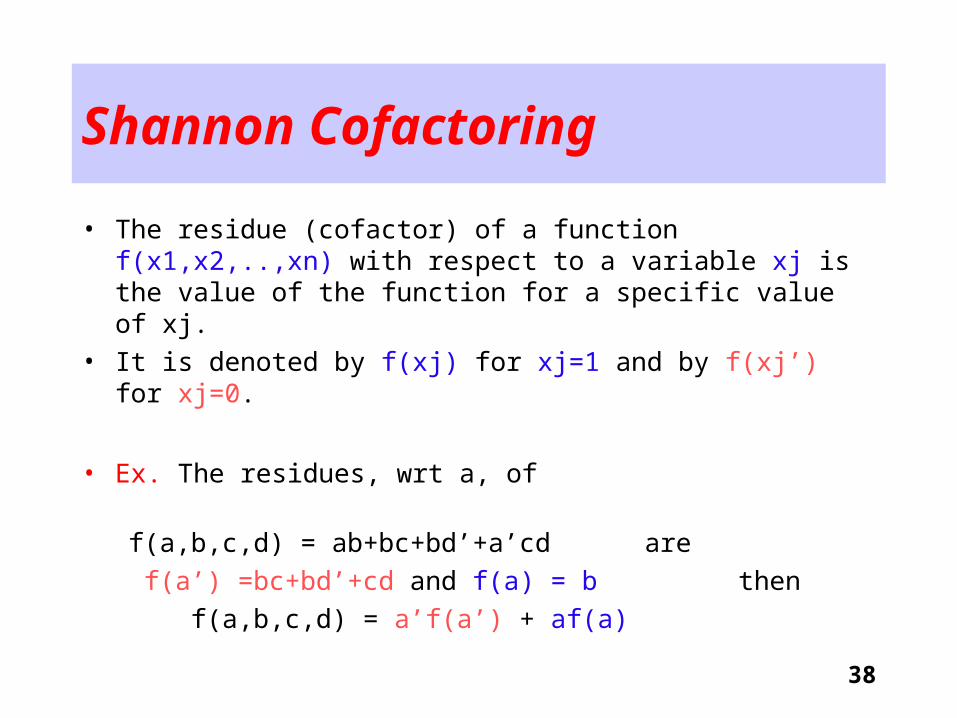
• The residue (cofactor) of a function f(x1,x2,..,xn) with respect to a variable xj is the value of the function for a specific value of xj.

• It is denoted by f(xj) for xj=1 and by f(xj’) for xj=0.

• Ex. The residues, wrt a, of

f(a,b,c,d) = ab+bc+bd’+a’cd are

f(a’) =bc+bd’+cd and f(a) = b then

f(a,b,c,d) = a’f(a’) + af(a)

39

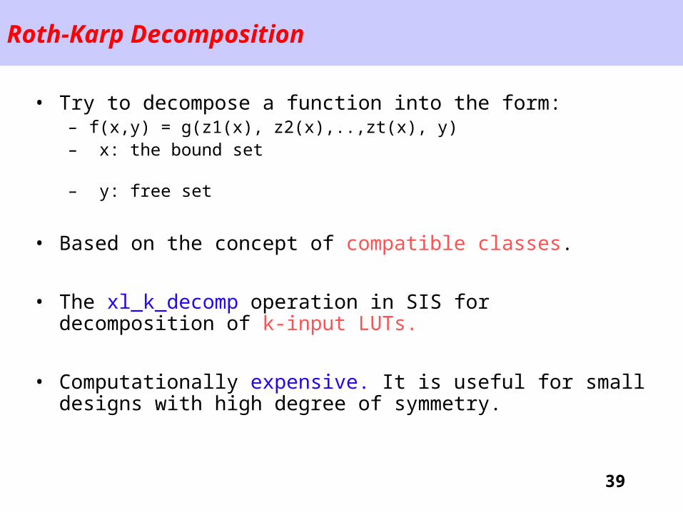
Roth-Karp Decomposition

• Try to decompose a function into the form: – f(x,y) = g(z1(x), z2(x),..,zt(x), y) – x: the bound set – y: free set

• Based on the concept of compatible classes.

• The xl_k_decomp operation in SIS for decomposition of k-input LUTs.

• Computationally expensive. It is useful for small designs with high degree of symmetry.

40

Algebraic Decomposition

• Based on factored form representation and algebraic operations.

• Manipulating algebraic expressions as polynomials; i.e., xi and xi’ are different variables.

• To reduce search, only common cube factors called kernels are used.

• Ex. x = ac+bc+bd+ce y = a+b+e and x = cy + bd

41

AND-OR Decomposition

• Ensure that any infeasible node is decomposed into a set of feasible nodes.

• Can be used to decompose large infeasible nodes into infeasible nodes that are small enough to make an exhaustive search for disjoint decomposition.

• Ex. F = ab+ac+bc can be decomposed into v=ab, w=ac, x=bc, y=v+w and z=y+x = F

42

Decomposition

– Decomposition consists of three steps:

• Identify divisors which are common to

many functions.

• Introduce the divisor as a new node.

• Re-express existing nodes using the new nodes.

43

An Example

• Given the expression

f = ab’+ac’+ad’+a’b+bc’+bd’+a’c+b’c+cd’+b’d+c’d

• Suppose a factor found is p = a+b+c+d

• f can be re-expressed based on p: f = p(a’+b’+c’+d’)

44

Decomposition TechniquesDecomposition Techniques

• Disjoint decomposition.

• Shannon cofactoring.

• Roth-Karp decomposition.

• Algebraic decomposition.

• AND-OR decomposition.

• I have slides about all these methods.

• I teach 3 different classes about them

45

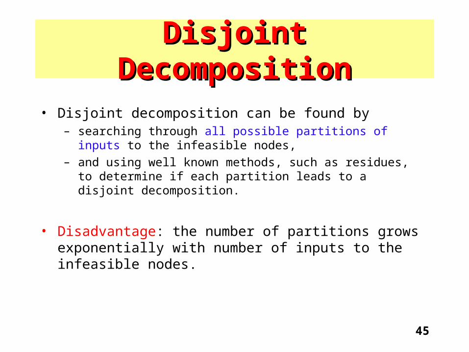
Disjoint DecompositionDisjoint Decomposition

• Disjoint decomposition can be found by – searching through all possible partitions of inputs to the infeasible

nodes,

– and using well known methods, such as residues, to determine if each partition leads to a disjoint decomposition.

• Disadvantage: the number of partitions grows exponentially with number of inputs to the infeasible nodes.

46

Functional DecompositionFunctional Decomposition

X

X

F

Y = F ( X )Y = F ( X )

A (U ) B (V )

G

H

47

Decomposition– typical procedures

a , b , c , . .. , f

F

f , f1 2

G

H

Transformacja

Dekompozycjawęzłów

f

f

1

2

x

y

y

vw

z

u

s

transformation

Decomposition of nodes

48

Algorithm for decomposition

X

Yg

Yh

R ó w n o l e g ł a

G H

Y

A B

X

S z e r e g o w a

G

H

Serial Parallel

49

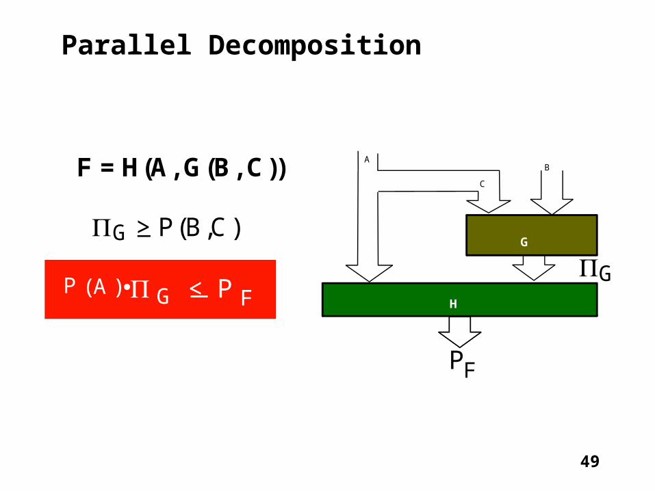
Parallel Decomposition

A

G

H

C

BF = H(A, G(B, C))

PG > P(B,C)

PGP ( A ) G FP < P

PF

50

Example of serial decomposition

x x x x x3 4 1 2 5

G

y y1 2

y3

H

x1x2x3x4x5 y1 y2 y3

1

2

3

4

5

6

7

8

9

10

11

12

13

14

15

0 0 0 0 0

0 0 0 1 1

0 0 0 1 0

0 1 1 0 0

0 1 1 0 1

0 1 1 1 0

0 1 0 0 0

1 1 0 0 0

1 1 0 1 0

1 1 1 0 0

1 1 1 1 1

1 1 1 1 0

1 0 0 0 1

1 0 0 1 1

1 0 0 1 0

0 0 0

0 1 0

1 0 0

0 1 1

0 0 1

0 1 0

0 0 1

0 0 1

0 0 0

1 0 0

0 1 1

0 1 0

0 0 1

0 0 0

1 0 0

51

Parallel Decomposition

X Y YHYG Y=

YHX H

YGX

GX G

F

XH

YHYG = FU

52

Example of parallel decomposition

y1 : {x1,x4}, {x4, x5}

y2 : {x2, x3, x5}

y3 : {x1, x4}

y4 : {x2, x5}, , {x5, x6},{x1, x6}

G = {y1, y3} H = {y2, y4}

Xg = {x1, x4} Xh = {x2 , x3, x5}

x1 x2 x3 x4 x5 x6 y1 y2 y3 y4 1 0 1 0 0 0 1 0 0 0 - 2 1 0 0 0 1 1 0 0 1 - 3 1 1 0 1 1 1 1 1 1 0 4 1 1 0 1 0 0 - 0 1 1 5 1 1 1 1 1 1 1 0 - 0 6 0 0 1 0 1 1 - 0 0 - 7 0 1 1 0 0 1 0 1 - 0 8 1 0 1 1 1 0 1 - 1 1 9 1 0 0 1 1 0 1 0 - 1

10 0 1 1 1 0 1 0 1 1 1

53

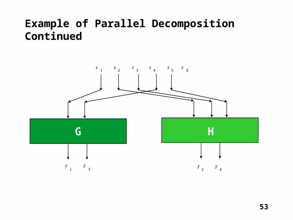
Example of Parallel Decomposition Continued

y y1 3

x x x x1 2 3 4

x x 5 6

y y2 4

G H

54

Balanced Method of Decomposition (Luba)

F

X

Y

Yg

h

Yh

gH

GX Xg X Xh

U U

Y Y = Yg h

SzeregowaRównoległa

U

UW

V

X

G

H

Parallel Serial

55

Method of puzzles

56

experimental results (1)

Porównanie ze względu na liczbę komórekName DEMAIN Chortle-

CrfASYL MIS FGSyn mulop

5xp1 9 20 13 17 9 9Alu2 47 83 60 84 55 51Clip 10 – 33 23 18 14

f51m. 8 – 14 11 8 8Misex1 8 14 13 9 8 9Misex2 24 – 24 23 22 24

rd73 5 – 8 7 5 5rd84 7 53 14 12 8 8sao2 16 – 30 28 25 20z4m1 4 3 4 6 4 49sym 5 – 8 7 – 7

Comparison of CLBs

57

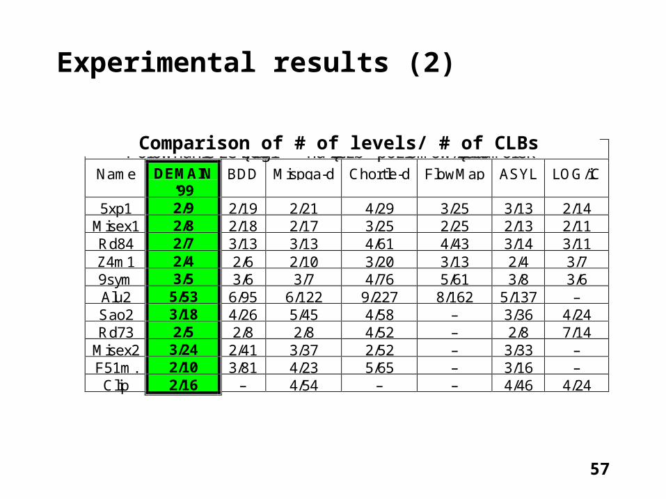
Experimental results (2)

Porównanie ze względu na liczbę poziomów/liczbę komórekName DEMAIN

‘99BDD Mispga-d Chortle-d FlowMap ASYL LOG/iC

5xp1 2/9 2/19 2/21 4/29 3/25 3/13 2/14Misex1 2/8 2/18 2/17 3/25 2/25 2/13 2/11Rd84 2/7 3/13 3/13 4/61 4/43 3/14 3/11Z4m1 2/4 2/6 2/10 3/20 3/13 2/4 3/79sym 3/5 3/6 3/7 4/76 5/61 3/8 3/6Alu2 5/53 6/95 6/122 9/227 8/162 5/137 –Sao2 3/18 4/26 5/45 4/58 – 3/36 4/24Rd73 2/5 2/8 2/8 4/52 – 2/8 7/14

Misex2 3/24 2/41 3/37 2/52 – 3/33 –F51m. 2/10 3/81 4/23 5/65 – 3/16 –Clip 2/16 – 4/54 – – 4/46 4/24

Comparison of # of levels/ # of CLBs

58

Experimental results (3)

Porównanie z systemem

MAX+Plus2

Name DEMAIN MAX+Plus2

9sym 10 98

Clip 19 404

Rd73 9 98

Root 37 113

Sao2 31 125

Z4 6 88

Comparison with MAX+Plus2 system

59

Two-bit adder – parallel-serial decomposition

x x x x x0 1 2 3 4

y y0 1

H2

x x x0 2 4

H1

y2

x x x x x0 1 2 3 4

F

y y y0 1 2

x x x x x1 3 0 2 4

G'

y y0 1

H2'

S = 105

60

y2

g g0 1

H 1

x x g1 3 1

y y0 1

H 2

x x x x x0 1 2 3 4

F

y y y0 1 2

x x x x x1 3 0 2 4

g g0 1

G

H

y y y0 1 2

S = 114

Two-bit adder – serial-parallel decomposition

61

Functional Decomposition

U V

H

G

G: bramki logiczneH: bez zmiany - tablica fr

Dekompozycja na bramki

U V

H

G

G: tablica typu frH: tablica typu fr

Dekompozycja klasycznaClassical Decomposition

Gate Decomposition

G: table of type fr

H: table of type fr

G: logic gates

H: no change – table of type fr

62

DES Algorithm

S1 S2 S3 S4 S5 S6 S7 S8

Permutacjaf(R,K)

Ekspansja PodkluczR32 48 48

32 32permutation

Sub-keyExpansion

63

Realisation of S-boxes using DEMAIN

S1 S2 S3 S4 S5 S6 S7 S8 TOTAL

DEMAIN 25 24 24 24 26 24 23 24 192

ALTERA 73 76 79 74 79 76 77 76 610

FLEX

FLEX DE MA IN

FLEXFLEX

64

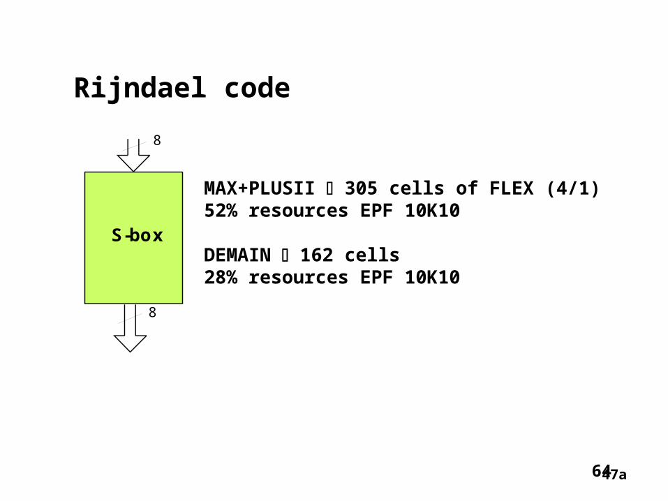
Rijndael code

S-box

8

8

MAX+PLUSII 305 cells of FLEX (4/1)52% resources EPF 10K10

DEMAIN 162 cells28% resources EPF 10K10

47a

65

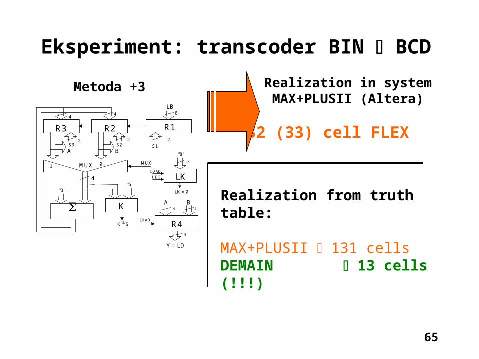
Eksperiment: transcoder BIN BCD

Y = LD

R4

K A B

LOAD

"3""5"

4

MUX 01

S3 S2A B

R3 R2

4 8LB

R12

MUX

LK = 0

4

"8"

LKLOAD

DEC

2 2

S1

K 5

44

8

4

Metoda +3 Realization in system MAX+PLUSII (Altera)

32 (33) cell FLEX

Realization from truth table:

MAX+PLUSII 131 cellsDEMAIN 13 cells (!!!)

66

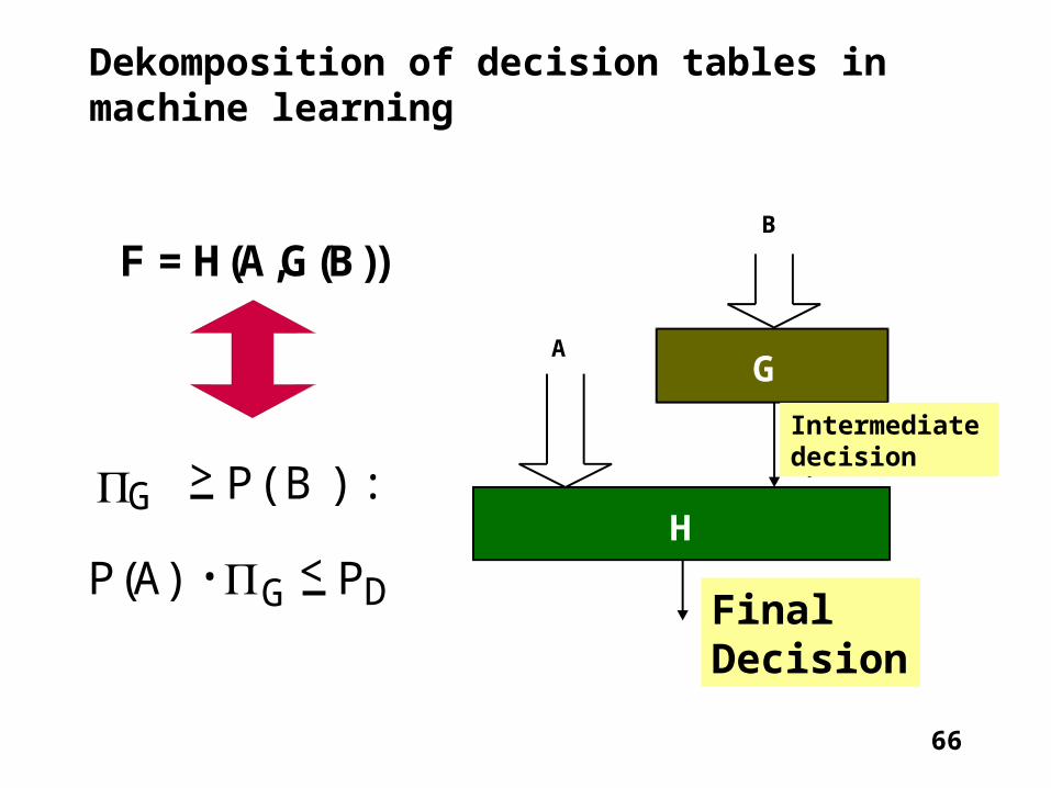
Dekomposition of decision tables in machine learning

A

B

G

H

D e c y z j a

k o ń c o w a

D e c y z j a

p o ś r e d n i a

P(A) < P . PG D_

PG > P( B ) :_

F = H(A,G(B))

Intermediate decision

Final Decision

67

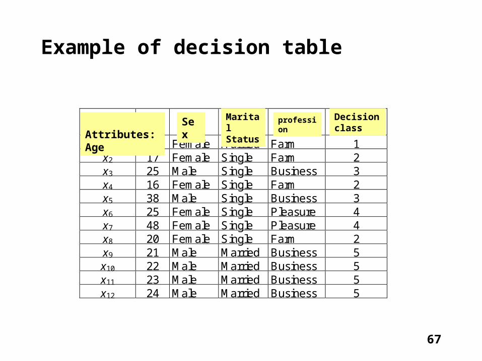
Example of decision table

Atrybuty: wiek płećStan

cywilnyzawód

Klasadecyzyjna

x1 20 Female Married Farm 1x2 17 Female Single Farm 2x3 25 Male Single Business 3x4 16 Female Single Farm 2x5 38 Male Single Business 3x6 25 Female Single Pleasure 4x7 48 Female Single Pleasure 4x8 20 Female Single Farm 2x9 21 Male Married Business 5x10 22 Male Married Business 5x11 23 Male Married Business 5x12 24 Male Married Business 5

Attributes: Age Sex Decision class

professionMarital Status

68

(Age, 20) (Marital_Status, Married) (Class, 1),(Age 16) (Class, 2),(Age, 17) (Class, 2),

(Age, 20) (Marital_Status, Single) (Class, 2),(Age, 25) (Gender, Male) (Class, 3),

(Age, 38) (Class, 3),(Age, 25) (Gender, Female) (Class, 4)

(Age, 48) (Class, 4),(Age, 21) (Class, 5),(Age, 22) (Class, 5),(Age, 23) (Class, 5),(Age, 24) (Class, 5).

Decision rules generated from a decision table

69

Example!, Decision table for house of reps. !,< D A A A A A A A A A A A A A A A A >!,[ CLASS-NAME HANDICAPPED-INFANTS WATER-PROJECT-COST-SHARINGADOPTION-OF-THE-BUDGET-RESOLUTION PHYSICIAN-FEE-FREEZE EL-SALVADOR-AID RELIGIOUS-GROUPS-IN-SCHOOLS ANTI-SATELLITE-TEST-BAN AID-TO-NICARAGUAN-CONTRAS MX-MISSILE IMMIGRATIONSYNFUELS-CORPORATION-CUTBACK EDUCATION-SPENDING SUPERFUND-RIGHT-TO-SUE CRIME DUTY-FREE-EXPORTS EXPORT-ADMINISTRATION-ACT-SOUTH-AFRICA ]!,!, Now the data!,democrat n y y n y y n n n n n n y y y yrepublican n y n y y y n n n n n y y y n y

republican n n y y y y n n y y n y y y n ydemocrat n n y n n n y y y y n n n n n y

. . . . . . . . . . . .

. . . . . . . . . . . . 68% kompresji danych68% Data compression

70

Decomposition-based FSM

A C B

G

register

H

F = H(A, G(B))

LUTs

EAB(s)

F = H(A, G(B C))

71

Synthesis Algorithm

1. Determine set A (preliminary encoding)

2. Determine partitions:

P(A), Pg = P(B)

3. Find partition Pg Pg

P(A) Pg PF

(eventually introduce set C)

4. Calculate functions G and H

72

FSM Synthesis - An example

a) I1 I2 I3 I5b) I1 I2 I3 I5

s1 s1 s2 s4 s1 1 2 3

s2 s5 s4 s2

4 5

s3 s3 s2 s1 s3 s3 6 7 8 9

s4 s2 s4 s1 s4 10 11 12

s5 s3 s1 s4 s2 s5 13 14 15 16

)4 ; 3,5,11,15 ; 6,9,13 ; 2,7,10,16 ; 1,8,12,14( PF

For s1 For s2 For s3For s4 For s5

First task is to find partition PF from state transition table

73

. . . Example, cont’d

I1 I2 I3 I4Final Encoding q1, q2, q3

s1 s1 s2 s4 s1 0 0 0

s2 s5 s4 s2 0 0 1

s4 s2 s4 s1 s4 0 1 0

s3 s3 s2 s1 s3 s3 1 1 1

s5 s3 s1 s4 s2 s5 1 0 1

Preliminary Encoding

)s,s ; s,s,s( 53421PSecond task is to find partition P from state transition table

This gives us variable q1

1. Determine set A

(preliminary encoding)

2. Determine partitions:

P(A), Pg = P(B)

3. Find partition Pg Pg

P(A) Pg PF

(eventually introduce

set C)

4. Calculate functions G and

H

74

. . . Example, cont’d

A = {x1, x2, q1} B = {q2, q3}

P(A)|PF = ((1)(6) ; (2) ; (3,7)(4) ; (5)(8) ; (9,13) ; (10)(14) ;

(11)(15) ; (12)(16))

Pg

1, 2, 3 6, 7 ,8

4, 5, 13, 14, 15, 16 9, 10, 11, 12

Hence: C = {x1}

)9,10,11,12; 6,7,8 ; 15,164,5,13,14, ; 1,2,3( PF

)s,s ; s,s,s( 53421P

75

Example, cont’d

B’ = {x1, q2, q3}

P(A)|PF = ((1)(6) ; (2) ; (3,7)(4) ; (5)(8) ; (9,13) ; (10)(14) ;

(11)(15) ; (12)(16))

)11,12 ; 9,10 ; 7,8 ; 6 ; 4,5,15,16 ; 13,14 ; 3 ; 1,2( P'g

)4,15,164,5,6,13,1 ; 9,10,11,121,2,3,7,8,(Pg

2131 xxqxg

In this new variant we create set B’

76

. . . Example, cont’d

x1 x2 q1

REGISTER

q1 q2 q3

G

H

x1

q2

q3

g

2131 xxqxg

77

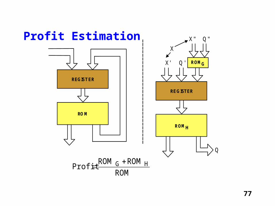
Profit Estimation

REGISTER

ROM

REGISTER

ROMH

ROMG

X" Q"

Q

X' Q'

X

ROM

ROMROMProfit HG

78

Materials used

GAL FLEX EPLD

ASIC

Tadeusz ŁUBA

Wydział Elektroniki i Technik Informacyjnych