NATIONAL COOPERATIVE HIGHWAY RESEARCH PROGRAM 1 28 REPORT

EVALUATION OF AASHO INTERIM GUIDES FOR

DESIGN OF PAVEMENT STRUCTURES

HIGHWAY RESEARCH BOARD NATIONAL RESEARCH COUNCIL

NATIONAL ACADEMY OF SCIENCES- NATIONAL ACADEMY OF ENGINEERING

HIGHWAY RESEARCH BOARD 1972

Officers

ALAN M. VOORHEES, Chairman WILLIAM L. GARRISON, First Vice Chairman

JAY W. BROWN, Second Vice Chairman W. N. CAREY, JR., Executive Director

Executive Committee

A. E. JOHNSON, Executive Director, American Association of State Highway Officials (ex officio) F. C. TURNER, Federal Highway Administrator, U.S. Department of Transportation (ex officio) CARLOS C. VILLARREAL, Urban Mass Transportation Administrator, U.S. Department of Transportation (ex officio) ERNST WEBER, Chairman, Division of Engineering, National Research Council (ex officio) D. GRANT MICKLE, President, Highway Users Federation for Safety and Mobility (ex officio, Past Chairman 1970) CHARLES E. SHUMATE, Executive Director-Chief Engineer, Colorado Department of Highways (ex officio, Past Chairman 1971) HENDRIK W. BODE, Professor of Systems Engineering, Harvard University JAY W. BROWN, Director of Road Operations, Florida Department of Transportation

W. J. BURMEISTER, Executive Director, Wisconsin Asphalt Pavement Association HOWARD A. COLEMAN, Consultant, Missouri Portland Cement Company

DOUGLAS B. FUGATE, Commissioner, Virginia Department of Highways WILLIAM L. GARRISON, Professor of Environmental Engineering, University of Pittsburgh ROGER H. GILMAN, Director of Planning and Development, Port of New York Authority

GEORGE E. HOLBROOK, E. I. du Pont de Nemours and Company GEORGE KRAMBLES, Superthtendent of Research and Planning, Chicago Transit Authority

A. SCHEFFER LANG, Department of Civil Engineering, Massachusetts Institute of Technology JOHN A. LEGARRA, Deputy State Highway Engineer, California Division of Highways WILLIAM A. McCONNELL, Director, Product Test Operations Office, Ford Motor Company JOHN J. McKETFA, Department of Chemical Engineering, University of Texas JOHN T. MIDDLETON, Deputy Assistant Administrator, Office of Air Programs, Environmental Protection Agency

ELLIOTT W. MONTROLL, Professor of Physics, University of Rochester R. L. PEYTON, Assistant State Highway Director, State Highway Commission of Kansas MILTON PIKARSKY, Commissioner of Public Works, Chicago DAVID H. STEVENS, Chairman, Maine State Highway Commission ALAN M. VOORHEES, President, Alan M. Voorhees and Associates ROBERT N. YOUNG, Executive Director, Regional Planning Council, Baltimore, Maryland

NATIONAL COOPERATIVE HIGHWAY RESEARCH PROGRAM

Advisory Committee

ALAN M. VOORHEES, Alan M. Voorhees and Associates (Chairman) WILLIAM L. GARRISON, University of Pittsburgh J. W. BROWN, Florida Department of Transportation A. E. JOHNSON, American Association of State Highway Officials F. C. TURNER, U.S. Department of Transportation ERNST WEBER, National Research Council D. GRANT MICKLE, Highway Users Federation for Safety and Mobility CHARLES E. SHUMATE, Colorado Department of Highways W. N. CAREY, JR., Highway Research Board

General Field of Design Area of Pavements Advisory Panel Cl-Il

H. T. DAVIDSON, Connecticut Department of Transportation (Chairman) W. B. DRAKE, Kentucky Department of Highways WILLIAM GARTNER, JR., Florida Department of Transportation J. H. HAVENS, Kentucky Department of Highways F. L. HOLMAN, JR., Alabama Highway Department W. R. HUDSON, University of Texas CARL L. MONISMITH, University of California

F. SHOOK, The Asphalt Institute

Program Staff

F. H. SCRI VNER, Texas A & M University P. G. VELZ, Minnesota Department of Highways A. S. VESIC, Duke University E. J. YODER, Purdue University STUART WILLIAMS, Federal Highway Administration J. W. GUINNEE, Highway Research Board L. F. SPAINE, Highway Research Board

W. HENDERSON, JR., Program Director LOUIS M. MAcGREGOR, Administrative Engineer WILLIAM L. WILLIAMS, Projects Engineer GEORGE E. FRANGOS, Projects Engineer HERBERT P. ORLAND, Editor JAMES R. NOVAK, Projects Engineer ROSEMARY S. MAPES, Editor HARRY A. SMITH, Projects Engineer CATHERINE B. CARLSTON, Editorial Assistant

NATIONAL COOPERATIVE HIGHWAY RESEARCH PROGRAM 128 REPORT

EVALUATION OF

AASHO INTERIM GUIDES FOR

DESIGN OF PAVEMENT STRUCTURES

C. J. VAN TIL, B. F. McCULLOUGH, B. A. VALLERGA,

AND R. G. HICKS

MATERIALS RESEARCH & DEVELOPMENT, INC.

OAKLAND, CALIFORNIA

RESEARCH SPONSORED BY THE AMERICAN ASSOCIATION

OF STATE HIGHWAY OFFICIALS IN COOPERATION

WITH THE FEDERAL HIGHWAY ADMINISTRATION

AREAS OF INTEREST:

PAVEMENT DESIGN

PAVEMENT PERFORMANCE

BITUMINOUS MATERIALS AND MIXES

CEMENT AND CONCRETE

MINERAL AGGREGATES

FOUNDATIONS (SOILS)

MECHANICS (EARTH MASS)

HIGHWAY RESEARCH BOARD DIVISION OF ENGINEERING NATIONAL RESEARCH COUNCIL

NATIONAL ACADEMY OF SCIENCES —NATIONAL ACADEMY OF ENGINEERING 1972

NATIONAL COOPERATIVE HIGHWAY RESEARCH PROGRAM

Systematic, well-designed research provides the most ef-fective approach to the solution of many problems facing highway administrators and engineers. Often, highway problems are of local interest and can best be studied by highway departments individually or in cooperation with their state universities and others. However, the accelerat-ing growth of highway transportation develops increasingly complex problems of wide interest to highway authorities. These problems are best studied through a coordinated program of cooperative research.

In recognition of these needs, the highway administrators of the American Association of State Highway Officials initiated in 1962 an objective national highway research program employing modern scientific techniques. This program is supported on a continuing basis by funds from participating member states of the Association and it re-ceives the full cooperation and support of the Federal Highway Administration, United States Department of Transportation.

The Highway Research Board of the National Academy of Sciences-National Research Council was requested by the Association to administer the research program because of the Board's recognized objectivity and understanding of modern research practices. The Board is uniquely suited for this purpose as: it maintains an extensive committee structure from which authorities on any highway transpor-tation subject may be drawn; it possesses avenues of com-munications and cooperation with federal, state, and local governmental agencies, universities, and industry; its rela-tionship to its parent organization, the National Academy of Sciences, a private, nonprofit institution, is an insurance of objectvity; it maintains a full-time research correlation staff of specialists in highway transportation matters to bring the findings of research directly to those who are in a position to use them.

The program is developed on the basis of research needs identified by chief administrators of the highway depart-ments and by committees of AASHO. Each year, specific areas of research needs to be included in the program are proposed to the Academy and the Board by the American Association of State Highway Officials. Research projects to fulfill these needs are defined by the Board, and qualified research agencies are selected from those that have sub-mitted proposals. Administration and surveillance of re-search contracts are responsibilities of the Academy and its Highway Research Board.

The needs for highway research are many, and the National Cooperative Highway Research Program can make significant contributions to the solution of highway transportation problems of mutual concern to many re-sponsible groups. The program, however, is intended to complement rather than to substitute for or duplicate other highway research programs.

NCHRP Report 128

Project 1-11 FY '68 ISBN 0-309-02009-3 L. C. Catalog Card No. 72-77531

Price $5.60

This report is one of a series of reports issued from a continuing research program conducted under a three-way agreement entered into in June 1962 by and among the National Academy of Sciences-National Research Council, the American Association of State High-way Officials, and the Federal Highway Administration. Individual fiscal agreements are executed annually by the Academy-Research Council, the Federal Highway Administration, and participating state highway departments, members of the American Association of State Highway Officials.

This report was prepared by the contracting research agency. It has been reviewed by the appropriate Advisory Panel for clarity, docu-mentation, and fulfillment of the contract. It has been accepted by the Highway Research Board and published in the interest of effective dissemination of findings and their application in the for-mulation of policies, procedures, and practices in the subject problem area.

The opinions and conclusions expressed or implied in these reports are those of the research agencies that performed the research. They are not necessarily those of the Highway Research Board, the Na-tional Academy of Sciences, the Federal Highway Administration, the American Association of State Highway Officials, nor of the individual states participating in the Program.

Published reports of the

NATIONAL COOPERATIVE HIGHWAY RESEARCH PROGRAM

are available from:

Highway Research Board National Academy of Sciences 2101 Constitution Avenue Washington, D.C. 20418

(See last pages for list of published titles and prices)

FOREWORD This report summarizes the most extensively used procedures for the design of struc-tural subsystems of highway pavements in the United States and contains recom-

By Staff mendations that have resulted in the concurrent publication by AASHO of the

Highway Research Board AASHO Interim Guide for Design of Pavement Structures. It is based primarily on

a review of the development and use of the "AASHO Interim Guide for the Design of Flexible Pavement Structures," distributed in October 1961, the "AASHO In-terim Guide for the Design of Rigid Pavement Structures," distributed in April 1962, and the research and experience accumulated by state highway departments subsequent to their distribution. Although this report will be of particular value to pavement designers as a supplement to the AASHO Interim Guide, it should also be

of considerable interest to all agencies and personnel involved in pavement design

and related fields.

Largely due to the complexity of the problem, the structural design of highway pavements has been an evolutionary process based primarily on the experience and judgment of highway engineers, augmented by empirical relationships developed by research and field studies. Performance of pavements nationwide over the past 50

years indicates that the subjective judgment of highway engineers has been rather successful. However, it is extremely difficult to translate the experience from a spe-cific group of conditions to a design problem involving different conditions. Also, it is not known with any degree of certainty whether pavements that have performed satisfactorily were constructed as economically as possible.

Although significant progress is being made toward more rational approaches to the structural subsystem design of over-all pavement system management, the alternate approach—emphasis on empirical techniques plus engineering experience and judgment—must continue to provide the basis for pavement design during the immediate future. The relationships between traffic loadings and structural com-ponents of conventional pavements developed during the AASHO Road Test have provided useful tools for improvement of empirical design procedures. The first re-ported use of Road Test results in pavement design procedures was described in

HRB Special Report 73. * Through its Subcommittee on Pavement Design Prac-tices, AASHO prepared Interim Guides for the design of flexible and rigid pave-ments. These were distributed to the state highway departments in 1962 for trial use. The objectives of this project were to (1) determine the use being made of the In-terim Guides by state highway departments and (2) develop proposed revisions to the Interim Guides based on the additional research and experience gained following

their distribution. After completion of the project and accomplishment of the objectives by Ma-

* Langsner, G., Huff, T. S., and Liddle, W. J., "Use of Road Test Findings by AASHO Design Committee." HRB Spec. Rep. 73 (1962) pp. 399-414.

terials Research & Development, Inc., of Oakland, Calif., and to provide state highway departments with maximum benefits from the study, an implementation phase of the study was initiated under a continuation contract with the same agency, the objective being the preparation of a draft copy of the AASHO Interim Guide for the Design of Pavement Structures, covering both flexible and rigid pavements, to be based on the proposed revisions to the previously unpublished Interim Guides. In addition to a review by the HRB advisory panel for the project, the draft of the AASHO Interim Guide prepared by Materials Research & Development was re-viewed and commented on by a special subcommittee appointed for this purpose by the AASHO Subcommittee on Roadway Design. The end result is the publication by AASHO of the AASHO Interim Guide concurrent with this report and based in large part on the recommendations contained in the report.

Attention is directed to the fact that current design practices of state highway departments are continually being modified. The initial effort on this report was completed in 1970, but its publication was deferred to provide for coordination with the AASHO Interim Guide and to allow for revisions resulting from work on the Guide. Efforts have been made to update the report in accordance with latest state highway department practices. Nevertheless, some individual current practices may not be completely in agreement with the information reported herein.

CONTENTS

1 SUMMARY

PART I

3 CHAPTER ONE Introduction and Research Approach

Objectives

Research Approach

Project Prosecution

Scope of Report

Glossary of Terms

5 CHAPTER TWO Findings

Summary of Current Design Practices

Significance Study

Idealized Design Procedure

19 CHAPTER THREE Recommendations

Significance Studies

Converting Mixed Traffic to Equivalent 1 8-Kip Single-Axle Loads

Structural Layer Coefficients

Soil Support

Regional Factors

Rigid Pavement Design

Overlay Design

37 CHAPTER FOUR Conclusions and Suggested Research

Conclusions

Recommended Future Research

39 REFERENCES

PART II

42 APPENDIX A Request for Information

60 APPENDIX B Current Research

63 APPENDIX C Supporting Information

103 APPENDIX D Procedure for the Resilient Modulus Test

104 APPENDIX E Alternate Significance Study

ACKNOWLEDGMENTS

The research reported herein was conducted under NCHRP Project 1-11 by Materials Research & Development, Inc., of Oakland, Calif. (now a Division of Woodward-Lundgren & Associates). B. F. McCullough (now at University of Texas), and C. J. Van Ti!, Vice President, served as co-principal inves-tigators. They were assisted by R. G. Hicks (now at Georgia Institute of Technology), and B. A. Vallerga, President, with the latter also serving as responsible administrative officer.

G. M. Williams and Emery Shaw of the Federal Highway Administration, played an integral part in the successful comple-tion of the project through their collaboration in the informa-

tion collection phase. Thanks are also extended to the many Regional and Divisional representatives of the FHWA and per-sonnel of the various highway departments for their valuable assistance and cooperation during this phase. Special thanks are extended to Emery Shaw for his specific suggestions and com-ments during preparation of the Request for Information form and the subsequent analysis.

Appreciation is also extended to Fred N. Finn for his initial input into the project and to Ian Scott and Phil Woods of the MR&D staff for their technical assistance.

EVALUATION OF AASHO INTERIM GUIDES FOR

DESIGN OF PAVEMENT STRUCTURES

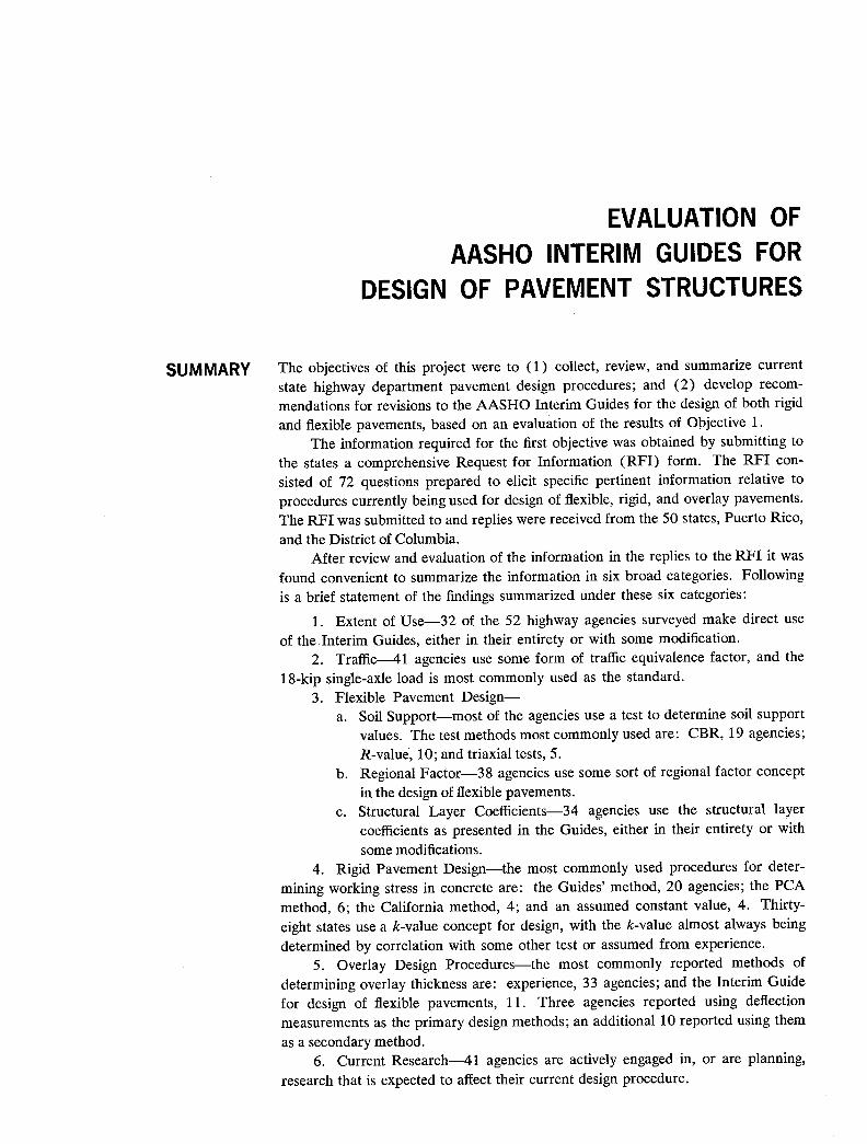
SUMMARY The objectives of this project were to ( 1 ) collect, review, and summarize current state highway department pavement design procedures; and (2) develop recom-mendations for revisions to the AASHO Interim Guides for the design of both rigid and flexible pavements, based on an evaluation of the results of Objective 1.

The information required for the first objective was obtained by submitting to the states a comprehensive Request for Information (RFI) form. The RFI con-sisted of 72 questions prepared to elicit specific pertinent information relative to procedures currently being used for design of flexible, rigid, and overlay pavements. The RFI was submitted to and replies were received from the 50 states, Puerto Rico,

and the District of Columbia. After review and evaluation of the information in the replies to the RFI it was

found convenient to summarize the information in six broad categories. Following is a brief statement of the findings summarized under these six categories:

1. Extent of Use-32 of the 52 highway agencies surveyed make direct use of the Interim Guides, either in their entirety or with some modification.

2. Traffic-41 agencies use some form of traffic equivalence factor, and the 1 8-kip single-axle load is most commonly used as the standard.

3. Flexible Pavement Design— Soil Support—most of the agencies use a test to determine soil support values. The test methods most commonly used are: CBR, 19 agencies; R-value, 10; and triaxial tests, 5. Regional Factor-38 agencies use some sort of regional factor concept in the design of flexible pavements. Structural Layer Coefficients-34 agencies use the structural layer coefficients as presented in the Guides, either in their entirety or with some modifications.

4. Rigid Pavement Design—the most commonly used procedures for deter-mining working stress in concrete are: the Guides' method, 20 agencies; the PCA method, 6; the California method, 4; and an assumed constant value, 4. Thirty-eight states use a k-value concept for design, with the k-value almost always being determined by correlation with some other test or assumed from experience.

5. Overlay Design Procedures—the most commonly reported methods of determining overlay thickness are: experience, 33 agencies; and the Interim Guide for design of flexible pavements, 11. Three agencies reported using deflection measurements as the primary design methods; an additional 10 reported using them

as a secondary method. 6. Current Research-41 agencies are actively engaged in, or are planning,

research that is expected to affect their current design procedure.

2

After analysis of the information contained in the summaries of the replies to the RFI, a significance study was conducted using the design procedures in the Guides for both rigid and flexible pavements in order to determine the relative influence of each of the variables. Also outlined was the idealized design procedure as originally developed from the results of the AASHO Road Test.

The specific and general recommendations developed are presented and dis-cussed under seven broad headings. Following is a brief statement of the scope and applicability of the recommendations made under each of these headings:

Significance Studies—these studies indicated that errors in some of the design parameters for both rigid and flexible pavements can result in designs that are excessively over- or underestimated. Research is needed to better quantify such factors as structural layer coefficients, soil support, regional factor, and vari-ance of flexural strength under field conditions, with the most immediate need being in the area of layer coefficients.

Converting Mixed Traffic to Equivalent 18-Kip Single-Axle Loads—because errors may result from using short-cut methods for converting mixed traffic to design traffic, it is recommended that the calculation method that gives the most accurate results from the available traffic data be used.

Structural Layer Coefficients—recommendations are made for the use of layered elastic theory to assist in developing appropriate structural coefficients for the component layers of flexible pavements.

Soil Support—layered theory is used to develop arational procedure for -correlating the-properties of local materials with the soil support scale in the Interim Guide for the design of flexible pavements. A theoretical analysis confirmed that this scale is reasonably valid.

Regional Factors—although the guidelines provided in the Guides are still valid and useful, it is recommended that research be conducted to obtain the information needed to develop better methods for establishing regional factors.

Rigid Pavement Design—recommendations are made for revision of the sections on materials properties, subbase, pavement thickness, reinforcement, and load-transfer devices in the Interim Guide for the design of rigid pavement. The recommendations are primarily for modifications of the existing approach to give more flexibility in analysis.

Overlay Design—it is recommended that the California method be adopted as an interim procedure for design of overlays for flexible pavements, and the U.S. Army Corps of Engineers method be adopted for rigid pavements.

CHAPTER ONE

INTRODUCTION AND RESEARCH APPROACH

One of the major objectives of the AASHO Road Test was to provide information that could be used in developing pavement design criteria and pavement design procedures. Accordingly, in May 1962, following completion of the Road Test, the AASHO Design Committee, through its subcommittee on Pavement Design Practices, reported in "The AASHO Road Test" (1) the development of the AASHO Interim Guides for the design of both rigid and flexible pavements (2, 3).* These Guides were based on the results of the AASHO Road Test, supplemented by existing design procedures and, in the case of rigid pave- ment, available theory. "The AASHO Road Test" stated:

It has been necessary, however, to make certain assump-tions in applying the Road Test equations to mixed traffic conditions and to those situations where soil materials and climate differ from those that prevailed at the test site.

These assumptions were necessitated by the fact that the performance equations from the Road Test were predicated on:

A specific set of paving materials and one subgrade. A single environment. An accelerated procedure for accumulating traffic

(two-year testing period to be extrapolated to 10- or 20-year designs).

Accumulating traffic on each test section by operating vehicles with identical axle loads and axle configuration (as opposed to mixed traffic).

The Interim Guides enumerate the assumptions and limitations associated with each design procedure, and each emphasizes that "the Guide is interim in nature and sub-ject to adjustment based on experience and additional research."

In 1962, the AASHO Committee on Design issued the Interim Guides to the states to be used for a one-year trial period with their existing procedures. The purpose of this trial period was to allow the states to review the design procedures, and to check their validity in actual practice. After the trial period, and subsequent receipt of comments by the states, the AASHO Committee on Design did not consider it necessary to revise the Guides or the instruc-tions at that time, and they were retained in their interim status.

While the Guides were under development, AASHO initiated a research program within NCHRP for the pur-pose of deriving a more theoretical pavement design method. Several NCHRP project goals are long-range in nature, compared to the more immediate aims of the

* Hereinafter referred to as Interim Guides or Guides. It should be noted that this project has resulted in the concurrent publication of the AASHO Interim Guide for Design of Pavement Structures (86) based on a review of the Interim Guides and recommendations for their revision reported herein.

AASHO Committee on Design. One NCHRP project (4, 5) developed guidelines for satellite studies of pavement performance that would extend AASHO Road Test results and strengthen the weaker areas of the Guides. However, relatively few such satellite studies were initiated by the states. A survey by Huff (6), on the use of satellite studies, revealed that 60 percent of the states replying to a ques-tionnaire had not initiated such studies, and that only a few of these states indicated such work would be considered in the future.

Because the possibility of acquiring data from a truly nationwide satellite study in the near future appeared to be remote, the NCHRP Advisory Panel Cl-il, on recom-mendation from AASHO, formulated this research project. Conceived as a practical alternative to the satellite study, it was to evaluate the various techniques used and the re-sults obtained by the individual states after applying the Guides to pavement structure design.

OBJECTIVES

In accordance with the Project Statement and subsequent working plan, this investigation had two basic objectives:

To collect, review, and summarize current state high-way department pavement design procedures.

To develop proposed revisions to the Interim Guides based on an evaluation of the results of Objective 1.

Inherent in these stated objectives is the need for evalu-ating the assumptions made in the Interim Guides and, where possible, to modify these assumptions on the basis of information available subsequent to the initial develop-ment of these Guides. Also essential to the project was a review of the Interim Guides to identify those factors and areas that were most significantly influenced by judgment, and for which Road Test data were lacking.

RESEARCH APPROACH

To accomplish the stated objectives, the project effort was divided into five major categories:

The study of available information and the prepara-tion of a request to the state highway departments for the additional information required.

A review of the information requirements with rep-resentatives of the Federal Highway Administration (FHWA; formerly the U.S. Bureau of Public Roads); NCHRP, and the AASHO Design Committee, and, through the cooperation of the FHWA, obtaining this information from the state highway departments.

A preliminary collating of information and analysis to formulate tentative revisions to the Interim Guides for

4

review by representatives of NCHRP, the AASHO Com-mittee on Design, and the FHWA.

A follow-up visit by the researchers to obtain addi-tional information, verify interpretations of previous in-formation obtained, and review the results of the pre-liminary analysis.

The final analysis and the preparation of the report with recommended revisions to the Interim Guides.

Two aspects of the project were considered critical in achieving the objectives. First, obtaining the required information from the state highway departments had to be on a person-to-person basis. This was accomplished through the excellent cooperation received from the FHWA. Second, the recommended revisions to the Interim Guides had to be based on realistic approaches with reason-able probability of acceptance by user agencies both at the state and federal levels. For this purpose, close coopera-tion and liaison with representatives of the FHWA and the AASHO Committee on Design was an integral part of this project.

PROJECT PROSECUTION

A Request for Information (RFI) form was prepared after a detailed study by the researchers of the Interim Guides, supplemented by a review of pertinent literature (7-20). A sample RFI form appears in Appendix A. The intent of the RFI was to obtain information relative to design procedures currently being used for design of flexi-ble, rigid, and overlay pavements. Speculative information as to the possible future orientation of the design procedure was not solicited.

The detailed attention given to the procedure used for obtaining the required information from various states on the RFI form was considered to be a major factor in ob-taining the 100 percent response. First, the FHWA trans-mitted copies of the RFI form to each regional and di-visional office. After each office had sufficient opportunity to study it, the Washington, D.C., office contact man personally called specific regional engineers to discuss the RFI, particularly with regard to interpretation problems that may have arisen. Concurrently, the researchers trans-mitted copies of the RFI form to all state highway engi-neers for referral to the appropriate design specialists. After the design specialists had studied the RFI, they fur-nished the requested information to a FHWA regional or divisional representative during a personal interview. The completed RFI's were collected by the Washington, D.C., office of the FHWA and transmitted to the researchers. Information was obtained from state highway departments of the 50 states, the District of Columbia, and Puerto Rico.

The researchers then collated, reviewed, and summarized the information from the 52 sources. This step fulfilled, in part, the intent of Objective 1. On evaluating this informa-tion, the researchers decided that maximum benefit for the time and money available for this study would be obtained by confining the scope of the study to the following areas:

1. A significance study of the parameters in the design equations to ascertain their relative effect on the final de-sign. Such information provides the designer with guidance

as to possible errors associated with assumed values, and, in effect, also provides weighting criteria for determining priority of research efforts.

An evaluation of the various methods for converting mixed traffic to equivalent wheel loads for use in design.

The development of a rational procedure for quanti-fying the soil support scale of the flexible pavement nomo-graph for conditions other than those at the AASHO Road Test.

The development of a rational procedure for quantify-ing the structural layer coefficients for local materials.

The development of criteria to assist each state in establishing regional factors that are compatible with the total system.

The development of a subbase design procedure that may be used with the rigid pavement equation to properly account for the increased supporting power obtained by treating the material.

The extension of the concepts for a pavement con-tinuity term and a reinforcement design in Appendices C and F of the Interim Guide for rigid pavements to provide the pavement designer a rational method for designing continuously reinforced concrete pavement.

The development of a procedure for evaluating the load-carrying capacity of an existing pavement structure, and using the information for developing overlay thickness requirements to provide for projected future traffic.

Based on the summarized information and on the fore-going major areas of study, eight states were selected for additional personal contact by the researchers. Criteria for selection of the states were the significance of probable inputs to the eight areas of study.

The states selected were California, Georgia, Illinois, Minnesota, North Carolina, Texas, Utah, and Virginia. Each state was visited by two researchers, with a list of questions regarding the background and the intent of one or more procedures of the state specifically applicable to the eight major areas of interest. The personal contact with state personnel also provided an opportunity to use them as a preliminary "sounding board" regarding possible revisions to the Interim Guides, and gave additional insight into problems associated with application of the Guides.

SCOPE OF REPORT

Chapter Two presents the findings of the study and is related primarily to Objective 1 in that the use of Guides is considered along with a summary of current practices. Also included are the significance study of the design parameters and a summary of current research by the states.

Chapter Three presents the recommendations for revis-ing and strengthening the Guides. Only specific recom-mendations are included; a detailed explanation of the development and the assumptions involved appears in Appendix C. This information is intended to fulfill the requirements of Objective 2. The conclusions and sug-gested research formulated as a result of this study appear in Chapter Four.

Appendix A includes the RFI form used and summary

tables, and Appendix B summarizes the status of on-going research. Appendix D contains information from the states relevant to the recommendations of Chapter Three. Appendix E contains information on the alternate sig-nificance study.

GLOSSARY OF TERMS

A glossary of terms used in this report follows: STRUCTURAL NUMBER (SN)—an index number derived

from an analysis of traffic, roadbed soil conditions, and regional factor that may be converted to thickness of various flexible pavement layers through the use of suitable layer coefficients related to the type of material being used in each layer of the pavement structure.

LAYER COEFFICIENT (a1, a0, a,)—the empirical relationship between structural number (SN) for a pavement struc-ture and layer thickness which expresses the relative ability of a material to function as a structural compo-nent of the pavement.

FLEXIBLE PAVEMENT LAYER THICKNESS (D1, D0 , D3)—thickness in inches of surface, base, and subbase courses, respectively, of a flexible pavement structure.

SOIL SUPPORT (S)—an index number that expresses the relative ability of a soil or aggregate mixture to support traffic loads through a flexible pavement structure.

REGIONAL FACTOR (R)—a numerical factor used to adjust the structural number of a flexible pavement structure for climatic and environmental conditions.

RIGID PAVEMENT SLAB THICKNESS (D)—thickness in inches of a portland cement concrete slab of a rigid pavement.

MODULUS OF SUBGRADE REACTION (k) —Westergaard's

modulus of subgrade reaction for use in rigid pavement design (the load in pounds per square inch on a loaded area of the subgrade or subbase divided by the deflection in inches, psi/in.).

MODULUS OF RUPTURE OF CONCRETE (S)-28-day flexural strength as determined by AASHO Designation T-97 using third-point loading.

WORKING STRESS IN CONCRETE (f)-0.75 times the modu-lus of rupture (S0).

TRAFFIC EQUIVALENCE FACTOR (e)—a numerical factor that expresses the relationship between a given axle load and an equivalent number of repetitions of an 1 8-kip single-axle load.

DAILY EQUIVALENT 1 8-xip SINGLE-AXLE LOAD APPLICATIONS

(W 18 )—the average daily traffic volume expected to pass a point or over a section of roadway during a given traffic analysis period that has been adjusted for lane and directional distribution and converted to equivalent 18-kip single-axle load applications.

TOTAL EQUIVALENT 1 8-sup SINGLE-AXLE LOAD APPLICA-

TIONS (W 18 )—the total traffic volume expected to pass a point or over a roadway section during a given traffic analysis period that has been adjusted for lane and direc-tional distribution and converted to equivalent 1 8-kip single-axle load applications.

PRESENT SERVICEABILITY INDEX (p)—a number derived by formula for estimating the serviceability rating of a pave-ment from measurement of certain physical features of the pavement.

TERMINAL SERVICEABILITY INDEX (Pt) —the lowest service-ability index that will be tolerated before resurfacing or reconstruction becomes necessary.

CHAPTER TWO

FINDINGS

Findings of this study are presented in summary form for each of the following areas: (1) the current pavement design practices of the 50 states, Puerto Rico, and the District of Columbia, (2) a significance study indicating the relative importance of the various design parameters of the Guides, and (3) idealized design procedure.

SUMMARY OF CURRENT DESIGN PRACTICES

On the basis of a review of available literature and the Interim Guides, a Request for Information (RFI) form was prepared and submitted to the 52 highway depart-ments. This RFI covered all aspects of pavement design, both flexible and rigid, and was designed to be completed by the engineers most familiar with each aspect of the

subject. The replies to the portion of the RFI relating to current practice were summarized, and are presented herein (see also Appendix A).

Of the 72 questions in the RFI, only certain specific questions were selected for inclusion in this summary.* Selection was on the basis of their special significance to current practice in design or rehabilitation of either flexible or rigid pavements.

Extent of Use

Table A-i is a summary of the extent of use of the Interim Guides in the 50 states, the District of Columbia, and

* Detailed information on questions not tabulated or reviewed in this report can be obtained from the FHWA.

6

Puerto Rico. In this table, use of the Interim Guides is given under four headings:

No direct use of the Guides. Have used the Road Test results to modify design

equations, but have not used the Guides. Have used the Guides as recommended by the

AASHO Committee on Design, in some cases with modification.

Are now in the process of obtaining information from field projects within the state that are expected to contribute to some modification and eventual use of concepts included in the Guides.

As Table A-i indicates, 32 of the 52 highway depart-ments surveyed make direct use of the Interim Guides, either entirely or with some modifications, in the design of pavement structures. More specific information as to how the states are using the Interim Guides follows.

Of the 20 states not currently using the Interim Guides directly, three are either conducting, or are planning to conduct, satellite studies in an attempt to adapt the Guides' design procedure to their use. In addition, a fourth state has modified its thickness design procedure for flexible pavements on the basis of the AASHO Road Test results.

Traffic

Of the replies to ten questions pertaining to the influence of traffic on the design of pavement structures, those to two questions were summarized to illustrate the methods cur-rently used to arrive at a numerical expression for traffic. The two questions were:

i. Q 2—Have you used the recommendations of the Interim Guides for establishing traffic equivalence factors for different wheel loads?

2. Q 4—What wheel or axle load is used to standardize the traffic equivalence factor?

Equivalence Factors

Table A-2 summarizes the response to Question 2. The replies are grouped into three categories:

Those states using the recommendations of the In-terim Guides for establishing traffic equivalence factors.

Those states using the FHWA modifications to the Interim Guides.

Those states not using Interim Guide traffic equiva-lence factors.

Note that 35 of the 52 highway departments use the Guides' traffic equivalence factor, either as recommended by the Guides or as modified by the FHWA. When the California equivalence factor concept is included, a total of 41 agencies use some form of equivalence factor con-cept. Comparing this table to Table A-i shows that three states (Kansas, Missouri, and Virginia) currently use the load equivalence concept, although they do not use the Guides to design pavements or to check their design.

Standard Wheel Load

Table A-3 is a summary of the response to Question 4. The replies are grouped into four categories for flexible pave-ments and three categories for rigid pavements.

For flexible pavement design, 38 highway departments use the 1 8-kip single-axle load, 8 use the California 5-kip wheel load, 4 use some other concept, and 2 do not consider load in their design.

For rigid pavement design, 23 highway departments use the 18-kip single-axle load, 17 use a form of the PCA design concept, 5 use standard sections, 2 base their designs on experience, and 5 do not use rigid pavements.

Soil Support Value

Of the replies to six questions in the RFI pertaining to soil, those to the following four questions were summarized:

i. Q 10—What method is used for evaluating the soil support value of the in-place material (e.g., CBR, R-value, Texas triaxial classification, modulus of subgrade reaction, swell pressure, etc.)?

Q 12—Have you used the guidelines set forth in the Interim Guides to incorporate soil support value into the design procedure?

Q 13—If so, how was the test procedure tied into soil support value?

Q 15—Do you have any correlations relating various standard test procedures (i.e., Stabilometer, CBR, k-value, etc.)?

Test Methods

Table A-4 is a summary of the response to Question 10. The replies are grouped into five areas:

States using the CBR test. States using the R-value test. States using some form of a triaxial test. States using the group index method. States using some method other than these four.

Twenty agencies use the CBR method for establishing soil support, 10 use the R-value test, 5 use a triaxial test, 6 use the group index, and ii use other methods for establishing the influence of soil on pavement design.

Table A-S gives a further breakdown of the methods used by the ii states included in the "other" column. The "other" methods are subdivided into six categories:

Other soil classification systems, such as AASHO, or some combination of liquid limit and gradation.

A pedological soil classification. A frost index system devised by the U.S. Army Corps

of Engineers. Experience. The use of standard sections.

In summary, 47 agencies use some form of laboratory test to define characteristics of the subgrade soil.

Incorporation into Design Method

Table A-6 is a summary of the replies to Question 12 regarding the methods used for incorporating soil support

7

into the pavement design procedure. The replies fall into three general categories:

Those agencies using the Interim Guides' recom-mendations for incorporating soil support into pavement design procedure.

Those agencies using the California method for incorporating soil support (R-value) into the pavement design procedure.

Those agencies using other methods.

Note that 31 agencies use the Guides' recommendations for incorporating soil support into pavement design pro-cedure, although all of these states do not use the Interim Guides for design. Of the 13 states that use other than the AASHO or California procedures, approximately half rely on experience to establish pavement design for different soil conditions.

Correlations Between Procedures

Table A-7 is a summary of the response to Question 15 regarding available correlations between different standard test procedures. The replies were grouped as follows:

CBR versus soil classification. CBR versus modulus of subgrade reaction (k-value). California resistance value (R-value) versus k-value. Other (specified by footnote). None.

Of the agencies, 28 indicated that they had no correla-tions available, although 2 of the 28 indicated that studies were under way to develop correlations. Of those indicat-ing availability of correlations, the most common were CBR versus k-value, with 6, and R-value versus k-value, with 9.

It should be noted that these relationships were not necessarily developed by the states for which they are shown. For example, CBR versus k-value relationships were developed by both the Portland Cement Association and the Corps of Engineers, whereas the R-value versus k-value relationship was developed by the California Division of Highways.

Regional Factors

Of the six questions in the RFI pertaining to procedures used to establish the effects of different environmental con-ditions on the performance of pavement structures, replies to the following four were summarized to provide an indication of the current status of the procedures:

Q 16—Have you used the guidelines set forth in the Interim Guides to establish a regional factor?

Q 18—Have you established any regional factors within your state or between states?

Q 19—What criteria were used to establish these regional factors?

Q 20—How do you account for frost penetration in your design procedure?

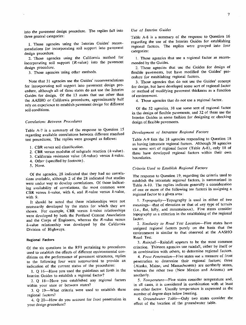
Use of Interim Guides

Table A-8 is a summary of the response to Question 16 regarding the use of the Interim Guides for establishing regional factors. The replies were grouped into four categories:

Those agencies that use a regional factor as recom-mended by the Guides.

Those agencies that use the Guides for design of flexible pavements, but have modified the Guides' pro-cedure for establishing regional factors.

Those agencies that do not use the Guides' concept for design, but have developed some sort of regional factor or method of modifying pavement thickness as a function of environment.

Those agencies that do not use a regional factor.

Of the 52 agencies, 38 use some sort of regional factor in the design of flexible pavements, and 32 of these use the Interim Guides in some fashion for designing or checking design of flexible pavements.

Development of Intrastate Regional Factors

Table A-9 lists the 18 agencies responding to Question 18 as having intrastate regional factors. Although 38 agencies use some sort of regional factor (Table A-8), only 18 of these have developed regional factors within their own boundaries.

Criteria Used to Establish Regional Factors

The response to Question 19, regarding the criteria used to establish the intrastate regional factors, is summarized in Table A-b. The replies indicate generally a consideration of one or more of the following ten factors in assigning a regional factor to a given area:

Topography—Topography is used in either of two meanings—that of elevation or that of any type of terrain (i.e., flat, hilly, and mountainous). Five states consider topography as a criterion in the establishing of the regional factor.

Similarity to Road Test Location—Five states have assigned regional factors purely on the basis that the environment is similar to that observed at the AASHO Road Test.

Rainfall—Rainfall appears to be the most common criterion. Thirteen agencies use rainfall, either by itself or in combination with others, to determine regional factors.

Frost Penetration—Five states use a measure of frost penetration to determine their regional factors; three (Alaska, Maine, and Massachusetts) are northerly states, whereas the other two (New Mexico and Arizona) are southerly.

Temperature—Five states consider temperature and, in all cases, it is considered in combination with at least one other factor. Usually temperature is expressed as the number of degree days below freezing.

Groundwater Table—Only two states consider the effect of the location of the groundwater table.

Subgrade Type—Four states use subgrade type in combination with some other factor.

Engineering Judgment—Thirteen of the states using regional factors rely solely on engineering judgment to arrive at a regional factor.

Type of Facility—Three states vary the regional fac-tor with type of facility or level of service. Generally, a higher regional factor is assigned to Interstate-type highways.

Subsurface Drainage—Five states consider drainage, either subsurface or surface, in determining regional factors.

Methods of Considering Frost Penetration

Table A-il is a summary of the response to Question 20 regarding methods for designing for frost penetration. The replies to this question are grouped into four categories:

Those states that consider frost effects to be a part of their regional factor.

Those states that call for a specific amount of non-frost-susceptible granular material.

Those states that do not consider frost effects in design.

Those states in which frost is not considered to be a problem.

Table A- il shows that 29 of the 52 agencies consider frost effects in some manner. --

Table A-12 summarizes the amount of non-frost—susceptible material required by agencies that consider frost in design. Note that the amount of such material required is based on a percentage of the depth of frost penetration, on the Corps of Engineers' procedure, or simply on experience.

Map of Regional Factors

Figure A-i shows a map summary of the regional factors used by agencies throughout the United States.

Structural Layer Coefficients

Six questions were included in the RFI to determine the use and application of the structural layer coefficient con-cept. Replies to the following three were selected for summarization:

Q 47—Are you using the structural coefficients recommended by the AASHO Interim Guide for deter-mining the structural number?

Q 50—What test methods are used to evaluate the structural coefficient of each layer?

Q 52—Do you vary the coefficient with position in the pavement structure?

Use of Guides

Table A-13 is a summary of the response to Question 47 regarding the use of the Interim Guides' structural co-efficients. The replies are grouped into four categories:

Use structural coefficients suggested by the Guides. Use these coefficients with some modifications.

Use these coefficients, but not for design. Do not use these coefficients.

Of the 52 agencies, 34 use the Guides either in their entirety or with some modifications.

For those agencies not using the Interim Guides' struc-tural coefficients, a further subdivision was made. Table A-14 summarizes the techniques used by these agencies in three groups:

Those using the California gravel equivalency concept. Those using other gravel equivalency concepts. Those using no equivalency concept.

As given in Table A-14, 9 of the 18 states that do not use the Interim Guides' structural coefficients assign some other equivalence factor to the materials of construction. Thus, 43 agencies use some technique to define the relative importance of a material in the pavement structure.

Table A-is summarizes (for each agency actively using the Guides) the coefficients or range of coefficients used for the pavement components. The components are listed as surface course, base course (untreated, cement-treated, lime-treated, and bituminous-treated), and subbase ma-terials. in general, the coefficients recommended by the Guides have been used with only minor modifications.

Test Methods Used to Evaluate Structural Layer Coefficients

Table A-16 summarizes the test methods used by eight states to evaluate the structural layer coefficient for sur-face, base, and subbase materials. Eight states actually evaluate or measure the structural coefficients through the use of some form of test procedure; of these, seven also vary the structural coefficient as a function of the test results. For further information on the procedures used, see Appendix C.

Variation of Coefficient with Position in the Pavement

Table A-17 summarizes the response to Question 52 re-garding the variation in structural coefficient with position. Of the agencies that employ the structural coefficient con-cept, 13 indicate that they vary the structural coefficient with position in the pavement structure. Of these states, most gave no precise indication of how or why they vary the structural coefficient. The available information is summarized in Table A-18.

Rigid Pavement

Of the 13 questions concerned with rigid pavement design, the replies to the following four were summarized:

Q 53a—In the Interim Guides it was recommended that the working stress in concrete be based on 0.75 of the modulus of rupture at 28 days based on AASHO T-97. What values are used in your design procedure?

Q 54a—How are the strength properties of untreated subbase evaluated? If by modulus of subgrade reaction (k), where is k determined?

Q 62a—Do you follow the Interim Guide design charts for percent steel in reinforced concrete pavements?

4. Q 63a—Are the Interim Guide design charts followed as regards percent steel in continuously reinforced concrete pavement?

Working Stress in Concrete

Table A-19 is a summary of the response to Question 53a regarding the method used to determine the working stress in the concrete. The replies are grouped into seven categories:

Use Guides' recommendations; i.e., working stress is equal to 0.75 times the modulus of rupture at 28 days.

Use California procedure; i.e., working stress is equal to 1.0 times the modulus of rupture at 28 days.

Assume a constant working stress based on experience for all jobs.

Use the Portland Cement Association (PCA) recom-mendations; i.e., working stress is equal to 0.50 times the modulus of rupture.

Use a standard structural section throughout the state. Rigid pavements not used, or no test method is used

and thickness is based on experience. Other test methods, including compressive strength

tests, are used.

Note that 20 agencies use the Interim Guides' recom-mendations, with the PCA method being second, with 6 users.

Determining Design k-Value

Table A-20 is a summary of the response to Question 47a on methods used to determine the modulus of subgrade reaction (k-value). Replies are grouped into seven categories:

Measure the subgrade k-value directly in the field. Assume a k-value based on previous experience. Obtain a k-value by correlation with the CBR test. Obtain a k-value by correlation with the R-value. Obtain a k-value by correlation with a triaxial test. Obtain a k-value by correlation with soil classification. Do not construct rigid pavements. Do not determine a k-value.

Reinforcement

Tables A-21 and A-22 are summaries of replies to Ques-tions 62a and 63a regarding conformance to the rec-ommendations in the Guides for reinforced concrete pavement (RCP) and continuously reinforced concrete pavement (CRCP). As indicated in Table A-21, 32 states use RCP, although only 18 of these follow the recommen-dations in the Guides. Table A-22 indicates that 19 states use CRCP and, of these, only 10 follow the Guides' recommendations.

Overlay Design Procedures

The RFI contains the following questions related to design of overlays:

1. Q 67—What procedure is used to evaluate the exist-ing pavement for purposes of estimating overlay require-

ments (e.g., experience, deflection, strain in surface course, or subgrade)?

Q 68—What tests and experience factors are used to evaluate properties of existing pavements?

Q 69—What are the required surface preparation requirements prior to overlay (e.g., subsealing, patching, or breaking the pavement)?

Q 70—What are the minimum requirements for over- lays (either flexible or rigid)?

The replies to these four questions follow.

Procedure Used

Table A-23 gives the response to Question 67 regarding the evaluation procedure used. The replies are generally ap-plicable to both flexible and rigid pavements, but a number are applicthle only to flexible pavements. Procedures used are grouped into five categories: deflection measurements; the Interim Guide for flexible pavements; AASHO Present Serviceability Index (PSI) concept; experience; and visual.

Although only 3 states use deflection as the primary evaluation procedure, 12 states consider it in some form, which is the same as the total using the Interim Guide for flexible pavements. The replies to questions pertaining to active research projects indicate a general interest among numerous states in using pavement deflection as a criterion for overlay design. California and Oklahoma have detailed procedures for using deflection to design overlays for exist-ing flexible pavements (43, 44). Oklahoma, in addition to deflection, also has procedures based on condition surveys and material properties. In general, the replies from the states indicate that the deflection evaluation has been de-veloped primarily for flexible pavements, with little use on rigid pavements.

The Interim Guide for flexible pavements (2) is being used to design flexible pavement overlays for existing flexi-ble and rigid pavements, but no attempt has been made to use the Interim Guide for rigid pavements (3) for this purpose. When one is using the Interim Guide for flexible pavements the overlay thickness is determined by sub-tracting the existing pavement structure thickness from the total thickness required by a new design. Each of the layers in the existing pavement is assigned a structural coefficient factor on the basis of experience. For existing rigid pavements, a structural coefficient of 0.3 to 0.4 is generally used.

The AASHO Present Serviceability Index (PSI) concept is largely a function of riding quality (45, 46). The AASHO PSI is being determined by combining surface roughness data obtained with instruments such as the CHLOE Profilometer or FHWA-type roughometers (16), and results of a condition survey of the amount of crack-ing and rutting. When the PSI drops below a prescribed level (generally a value of 2.5) an overlay of asphaltic concrete is added to restore the riding quality. The con-cept does not include load-carrying capacity of the pave-ment, and other means, such as the Interim Guide for flexible pavements, must be used to determine the thick- ness of overlay required.

The "experience" classification is further subdivided into

10

"rideability" and "pavement condition surveys," and given in Table A-24. Riding quality is generally measured by the CHLOE Profilometer (16), the FHWA-type rough-ometer (16), or the Portland Cement Association road-meter (47). More than nine states have purchased the CHLOE Profilometer, but evidently a number of these states have used it as a research tool only. Other states, such as California, use a profilometer for construction control, but not for maintenance (48). Condition surveys involve some measure of one or more of the follow-ing indications of distress: various cracking patterns by type, spalling, rutting, faulting, pumping, and general deterioration.

Experience Factors Considered

The replies to Question 68, as summarized in Table A-25, indicate that seven factors are considered: condition sur-vey, riding quality, maintenance cost, materials survey, traffic, skid resistance, and deflection. These seven factors encompass most of those recommended in the pavement systems analysis developed as a part of NCHRP Project 1-10 (49). In terms of a systems analysis, the condition survey, materials survey, and deflection are measures of performance, whereas riding quality, maintenance cost, traffic, and skid resistance are decision criteria for judging performance.

The most commonly reported of these factors are riding quality, with 19, and pavement condition surveys, with 20. Only four states give specific consideration to maintenance costs. One possible explanation for this is that pavement structure maintenance costs are difficult to separate from other maintenance costs (such as grass mowing, salting, light standards, and signs) in the maintenance logs of most states.

Ten agencies reported that they make a material survey of the project to determine properties of the subgrade and the component parts of the pavement structure. Of the seven factors given in Table A-25, only a materials survey or a deflection survey will provide data for evaluating the load-carrying capacity of a pavement structure. Because 4 of the 10 agencies using material surveys also make deflection surveys, only 18 report making an evaluation of the in-place pavement structure.

The consideration of traffic factors involves a projection of average daily traffic or total axle loads. Of the 18 states reporting as considering traffic, 12 indicated they used the Interim Guide for flexible pavements. This correlation is understandable because the use of the Guides requires an estimate of total equivalent wheel loads for the design period. Usually an 1 8-kip equivalent single-axle load is used as the standard.

Skid resistance represents a decision criterion for judging performance. Although three states reported this factor as being considered, levels of skid resistance considered unacceptable were not given.

Minimum Overlay Thicknesses

The reported minimum requirements for overlay thick-nesses for structural improvement are given in Table A-26.

These are not necessarily absolute values, as they may be varied based on project conditions. Several of the states also reported minimums for skid resistance improvement, generally based on construction equipment limitations rather than on design. With regard to overlays with portland cement concrete, only North Carolina and Texas have established minimums. The Texas Highway Depart-ment minimums are applicable only to CRCP overlays, because this is the only concrete pavement type that has been used for overlay construction.

Current Research

Table A-27 summarizes the reported status of current research activity relative to pavement design in the 50 states and two districts. As indicated, 36 agencies are actively engaged in or are planning research that is expected to affect their current design procedures. Table A-28 gives a breakdown of the type of research being pursued. Re-search activity falls into 19 categories where two or more states are involved. The following seven areas of major concentration are ordered in terms of number of states:

Soil or base stabilization—lO states. Development of structural coefficients-7 states. Correlation with Road Test results-6 states.

-4. Mix design—both flexible and rigid-6 states. Maintenance considerations (overlay design proce-

dures)-5 states. Performance studies-5 states. Properties of base and subbase materials-4 states.

For additional details on the type of research being conducted see Appendix B.

SIGNIFICANCE STUDY

In the design equations for flexible and rigid pavement structures, the thickness structural number (SN), for flexi-ble pavements, and slab thickness (D), for rigid pavements, are expressed as functions of several design parameters. These design parameters are of a stochastic nature, and potential variations in each parameter must be recognized by the pavement designer. More important to the designer, however, is the effect that variations in each of the pa-rameters have on the resultant thickness term SN or D.

The objectives of this study are:

To evaluate the relative importance of each parame-ter in the AASHO design procedures for flexible and rigid pavements.

To determine the change in structural number (SN) for flexible pavements and slab thickness (D) for rigid pavements that would result from an error in each of the design parameters.

To provide an indication of the area (or areas) where research would be most effective for future improvements to the Gides.

Approach

The significance study described herein consists of deter-mining the change in the dependent variable (SN or D)

11

resulting from a unit change in an independent design parameter (or variable). Design Eqs. 1 and 2

- 018 -

— (1 O0.b0 GP] SN

I

1.05 1W p0.1060

00 019 T( 3) ) ( l /

and

/ 1.019W0180'36

D°•75 - 1.132 )]4.22-0.32p,

D = l00.136G/[( D°75 - ZO.25

) ( 2)

were used as a basis for this study; all the terms are as described in the Glossary of Terms. Each equation was programmed into a 6400 CDC computer and the thick-ness was computed over a range of assumed errors in the design parameters.*

The change in SN or D resulting from an assumed error in the design parameters considered were computed at three levels for each parameter and at three levels of error magni-

* An alternate significance study with traffic as the dependent variable was also conducted and details are found in Appendix E.

TABLE 1

FACTORIAL FOR ERROR ANALYSIS IN TERMS OF STRUCTURAL NUMBER, SN, FLEXIBLE PAVEMENTS

tude. The magnitudes of each parameter considered are given in factorial form in Tables 1 and 2 for flexible and rigid pavements, respectively. Where possible, one level for each parameter corresponded to conditions representa-tive of those found at the AASHO Road Test. The three levels of error selected for most of the analysis were ±1, 5, and 10 percent of an average range of each variable. For two parameters, concrete flexural strength and concrete modulus of elasticity, a value of 20 percent was used instead of 10 percent, because each of these has a greater potential variability under field conditions. The terminal serviceability index (Pt) was assumed as 2.5 in all cases.

Using a computer, Eqs. 1 and 2 were solved at each combination of design parameters given in Tables 1 and 2. These data were then plotted on graphs to show the re-sultant change in SN or D caused by an induced error in each parameter. The percent error in SN or D was computed as follows:

Ej (T(Ji± (3)

Tj

)_T3

in which

E0 = percent change in the design structural number (SN) or slab thickness (D) due to a variation in the design parameter i;

T. = design thickness (SN or D) for the fac-torial; j indicates block of factorial listed in Tables 1 and 2; and

TABLE 2

FACTORIAL FOR ERROR ANALYSIS IN TERMS OF SLAB THICKNESS, D, RIGID PAVEMENTS

4 .r

3 6 10

10 6 5.5

10 7

10

1.0 106

10

10

5.0 106

107

loOs_

60

- 400 a

1000

65

400

4.

1005

60

400

1000

12

T(j, i ± z) = design thickness for factorial block I with assumed error ± A in parameter i.

A positive value of E indicates a resultant increase in the pavement thickness term, whereas a negative value indicates a decrease.

Flexible Pavements

The percentage change in SN was calculated for each of the 27 factorial cells at the indicated errors in regional factor (R), soil support (5), and traffic (W118 ). In each cell, 19 independent solutions were made—one at the actual value plus six each at the plus and minus variations about the three parameters, for a total of 513 solutions.

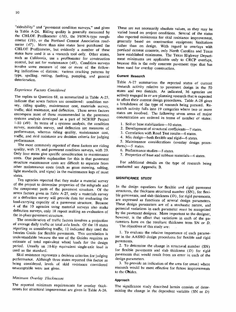
Regional Factor (R)

The percentage error in SN resulting from variations in regional factor (R) is shown in Figure 1. The change is positive for an increase and negative for a decrease in the parameter R. The results indicate that a plus or minus error in R has the same effect on SN and that, for a given error in R, the change in SN increases as the magnitude of R decreases. For example, if a pavement were designed for a regional factor of 0.5 and subsequent calculations indi-cated R to equal 1.0 (an error in R of 0.5), the change in SN would be about 14 percent. At all levels, the change in SN that results from an error in R is independent of the soil support and traffic.

Soil Support (5)

The percentage change in SN for any error in the soil support value is shown in Figure 2. The change is positive if S is underestimated and negative if S is overestimated. The results show that the change in SN is independent of the design parameters R and W 18 and slightly dependent on the magnitude of S. Regardless of whether the error in S is plus or minus, it has the same relative effect on changes to SN.

Traffic (W118 )

Figure 3 shows the change in SN with an error in the number of equivalent 1 8-kip single-axle loads. The change in SN due to an error in traffic is independent of the design parameters S and R and dependent on the level of traffic. For the curves representative of 1 million and 10 million load applications, a plus or minus error in traffic results in the same change in SN. The curve representative of 100,000 load applications is for a plus error only.

Discussion of Results

Of the three variables considered, an error in the design traffic number has the most pronounced effect on SN for 100,000 total equivalent 18-kip axle loads. Next in order are soil support and regional factor, although the two have approximately equal influence. An error in the design traffic number has little effect on SN when total load applications exceed 10 million. The combined effect of error in all three design parameters can be expressed as:

(E7,) cN =E1V+ES+ER (4)

in which

(Er) SN = total percentage change in SN resulting for

errors in estimating design parameters W 18 ,

S, and R; E jv = percentage change in SN due to errors in

parameter W 18 ;

Es = percentage change in SN due to errors in parameter S; and

ER = percentage change in SN due to errors in parameter R.

The following example problem shows the meaning of Figures 1, 2, and 3:

ERROR IN PARAM-

VALUE TERMS OF ETER ERROR

PARAM- PARAMETER ERROR INSN

ETER ASSUMED ACTUAL UNITS (%) (%)

R 0.75 1.0 +0.25 25 —4.0 S 3.0 2.5 —0.5 20 —6.5 W 18 1 x 105 2 X 10 +105 50 —16.0

—26.5

For the assumed or design parameters, a structural num-ber of 2.62 is required; however, because of incorrect esti-mate of traffic, regional factor, and soil support, the pave-ment was actually underdesigned by 26.5 percent or by 0.69 SN units. This could result in one of the following thickness errors:

LAYER THICKNESS

MATERIAL COEFFICIENT (IN.)

Asphaltic concrete 0.44 1.57 Aggregate base 0.14 4.95 Aggregate subbase 0.11 6.3

This problem demonstrates the usefulness of the sig-nificance study. However, any other combination of error values may be used with Figures 1, 2, and 3 to evaluate their influence on SN.

Rigid Pavements

The percentage change in slab thickness, D, was evaluated for each of the 81 factorial cells of Table 2 for the indi-cated errors in flexural strength, subgrade modulus, modu-lus of elasticity, and traffic. In each cell, 25 independent solutions were made—one at the actual value plus six each at the plus and minus variations about the four design variables, for a total of 2,025 solutions.

Flexural Strength (Se)

The change in D due to variations in fiexural strength is shown in Figure 4, where the percentage change in D

13

20

20

SOIL SUPPORT 3, 6, 10

TRAFFIC = iø, 106 , 10 7 04

REGIONAL FACTOR = 0.5, 1.0, 5.0

TRAFFIC = io, 106, 1 7

R = 0.

R = 1.

2 0 7

15

04 0

0 I-

10

04 0 04 04

2 U 04 5

0.

S = 10

S3

S6

0 = 5.

0 2 4 6 8 10 0 2 4 6 8 10

PERCENT ERROR IN REGIONAL FACTOR RANGE PERCENT ERROR IN SOIL SUPPORT RANGE

I I I

0

I I

0.1 0.2

I I I I

0.3 0.4 0.5

I I I

0 0.2 0.4 0.6 0.8 1.0

ERROR IN REGIONAL FACTORS UNITS ERROR IN SOIL SUPPORT UNITS

Figure 2. Effect of soil support variations on structural number. Figure 1. Effect of regional factor variations on structural number.

60

50

2 0 z - 40

0

30 z

0 0 04 04

20 z

04

10

40

40 30

U

TRAFFIC = 10, 10 6, 10 7

SUBGRAOE MODULUS = 60, 400, 1000

MODULUS OF ELASTICITY 0 10 6, 4.2X106, 6X106

20

40 z I

2

10

0-

It w 0 10 15 20

18 PERCENT ERROR IN FLEXURAL STRENGTH RANGE

0 120

ERROR IN FLEXURAL STRENGTH UNITS PERCENT ERROR IN TRAFFIC RANGE

I I I I I I Figure 4. Effect of flexural strength variations on slab thickness.

0 2X105 4I105 6X10 5 8X10 106

ERROR IN TRAFFIC UNITS

Figure 3. Effect of traffic variations on structural number. Traffic (W118 )

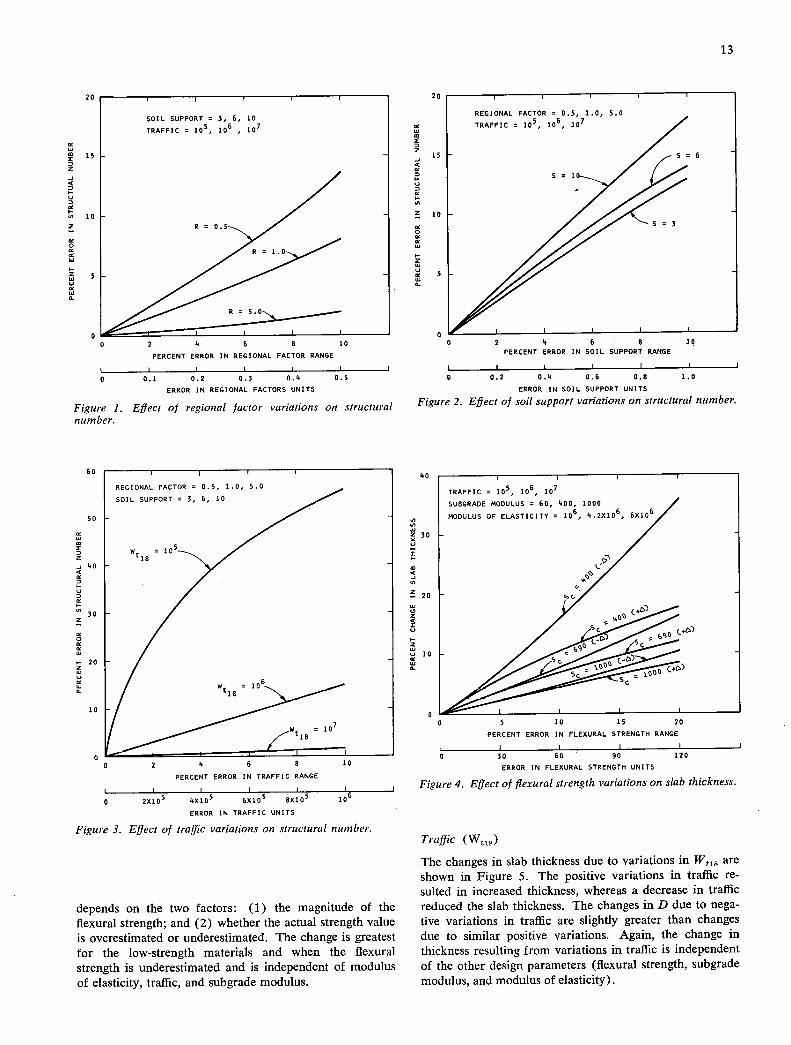
The changes in slab thickness due to variations in W 18 are shown in Figure 5. The positive variations in traffic re-sulted in increased thickness, whereas a decrease in traffic

depends on the two factors: (1) the magnitude of the reduced the slab thickness. The changes in D due to nega-

ulexural strength; and (2) whether the actual strength value tive variations in traffic are slightly greater than changes is overestimated or underestimated. The change is greatest due to similar positive variations. Again, the change in for the low-strength materials and when the flexural thickness resulting from variations in traffic is independent strength is underestimated and is independent of modulus of the other design parameters (flexural strength, subgrade of elasticity, traffic, and subgrade modulus. modulus, and modulus of elasticity).

20

14

60

50

0 -

FLEXURAL STRENGTH 400, 690, 1000

SUBGRADE MODULUS 60, 400, 1000

MODULUS OF ELASTICITY = 10, 4.2X106, 6X106

w 10 t18

, , w 106

t iE

, / W t18

106 ) -, 7- -

FLEXURAL STRENGTH 400, 690, 1000

TRAFFIC r 10, 10 6,

MODULUS OF ELASTICITY = 10 6 4.2X106, 6io6,r

/ /

/ /

k = 60

/ /

/

k = 60

400

k - 1000

0 2 4 6 8 10

18

PERCENT ERROR IN SUBGRADE MODULUS RANGE

2 4 6 8 10

PERCENT ERROR IN TRAFFIC RANGE

0 2X10 4010 6X105 8X105 106

ERROR IN TRAFFIC UNITS

Figure 5. Effect of traffic variations on slab thickness.

Modulus of Subgrade Reaction (k)

The changes in pavement life due to variations in the k-value depend on the level of traffic, modulus of elasticity, and flexural strength. In general, the percentage change in D increases with decreasing traffic, increasing flexural strength, and decreasing modulus of elasticity. Average curves for each level of subgrade reaction are shown in Figure 6. For the low level of subgrade reaction, a nega-tive error in k induces a greater change in D than a cor-responding positive error. At the higher levels of k, the negative or positive error results in similar changes in slab thickness.

Modulus of Elasticity (E)

The change in slab thickness is positive for an increase and negative for a decrease in the modulus of elasticity of the concrete. The percentage change in thickness due to varia-tions in modulus is shown in Figure 7. These data indicate that the change depends on the concrete modulus and is independent of subgrade modulus, flexural strength, and traffic.

Discussion of Results

As in the case for flexible pavements, of the four variables considered, an error in the design traffic number has the most significant effect on the slab thickness for 100,000 total equivalent 18-kip axle loads. Next in order are flexural strength, modulus of elasticity, and subgrade re-action. An error in the design traffic number has little effect on D when total load applications exceed 10 million.

0 20 40 60 80 180

ERROR IN SUBGRADE MODULUS UNITS

Figure 6. Effect of subgrade modulus variations on slab thick-ness.

The combined effect of errors in all four design pa-rameters on the resultant slab thickness can be expressed as:

(ET) fl =ElI+Es+Ek+EE (5)

in which

(ET ) = total percentage change in D resulting from errors in estimating design parameters W 15 , Sc, k, and E;

E31. = percentage change in D due to error in pa-rameter W 18 ;

E26 = percentage change in D due to error in pa-rameter S;

E1 = percentage change in D due to error in pa-rameter k; and

EE = percentage change in D due to error in pa-rameter E.

The following example problem shows the meaning of Figures 4, 5, 6, and 7.

ERROR IN PARAM-

VALUE TERMS OF ETER ERROR

PARAM- PARAMETER ERROR IND ETER ASSUMED ACTUAL UNITS (%) (%)

S 690 630 —60 10 —8.0 W 18 106 2 X 106 +106 50 —13.0 k 100 60 —40 67 —3.0 E 4.2 X 106 4.7X 106 +500,000 10 —2.2

—26.2

For the assumed or design parameters a slab thickness of 7.5 in. would be required; however, due to poor construc-

15

z

I-

-J 10

z

z .c I

z 5

tion control and estimates of traffic and other parameters, the slab thickness is actually underdesigned by 26.2 percent, or about 2 in.

Conclusions

This study was conducted to determine the sensitivity of the structural thickness terms SN, for flexible pavements, and D, for rigid pavements, to possible errors in each pave-ment design variable. The findings are limited to the range of variables investigated and for Eqs. 1 and 2. These find-ings however, provide the engineer with information with respect to the design parameter(s) that require(s) the most study to reduce possible over- or underestimates of the design thickness terms.

IDEALIZED DESIGN PROCEDURE

This section develops an idealized format for using the Interim Guides to design the pavement structure required for a given facility. From the response to the nationwide survey of states and from personal conversations with state personnel it is evident that the shortcut steps presented in the Guides are being used by most states, and that, in some cases, even further simplifications have been adopted. Thus, the more complete, or idealized, design procedures pre-sented in the Guides are seldom used.

The design equations used in the Guides were derived from mathematical models developed at the AASHO Road Test and expressing traffic applications as a function of layer thickness, layer properties, axle load, axle type, and terminal serviceability level. These equations are empiri-cal models that were statistically fitted to the Road Test data to give the smallest error of estimate. When these equations are used as originally derived (i.e., with traffic as the independent variable) they are in a closed form that may be solved directly for traffic. However, the highway pavement designer is generally interested in solving for the required structural number or for pavement thickness. Be-cause the AASHO equations cannot be expressed in terms of structural number or pavement thickness in a closed form, an iterative procedure must be used in solving the equations.

In the Interim Guides, nomographs were prepared for ease in solving the equations. However, most states use the average values of traffic equivalence factors presented in the text of the Guides to compute the required pavement structure without iteration, thus ignoring the fact that traf-fic equivalencies vary with structural number and terminal serviceability, as well as with axle load. The idealized design procedure as originally intended for use with the Guides is outlined in the following, together with recom-mendations for improving the procedure.

General Format

Figure 8 is a flow chart for the idealistic design procedure originally conceived for the Guides. This chart was de-veloped for computing structural number, but the same principles are also applicable to computing concrete pave-ment thickness with the Interim Guide for rigid pavements. The input values on the chart are: predicted traffic in

15

FLEXURAL STRENGTH = kOO, 690, 1000

TRAFFIC = io, 106, io SUBGRADE MODULUS = 60, 400, 1000

E = 16

E = *.2X10

6X106

5 10 15 20

PERCENT ERROR IN MODULUS OF ELASTICITY RANGE

0 2.5X10 5X105 7.5X105 10

ERROR IN MODULUS OF ELASTICITY UNITS

Figure 7. Effect of modulus of elasticity variations on slab thickness.

terms of wheel load data, the value of soil support, and the regional factor. A structural number is assumed and used with the input data to ascertain the proper traffic equivalence factors to use for computing the total 18-kip

I ASSUME SN I

PREDICTED

TRAFFIC & WHEEL LOAD I COMPUTE LOAD DATA I EQUIVALENCIES

CONVERT MIXED

TRAFFIC TO TOIAL EWL

DESIGN LUE3 FOR

I. SOIL SIWPORT COMPUTE SN

2.REGIONAL E.CTOR

COMPARE COMPUTED SN AND ASSUIitD SN

YES

DESISN SN

Figure 8. Flow chart for idealistic procedure for computing required SN.

16

single-axle loads expected. After the total equivalent wheel loads are computed, the next step is to compute the re-quired structural number using the soil support and re-gional factor data. This step is an iterative process sub-system, discussed later.

After the required structural number is computed, the value is compared with the assumed structural number in terms of some acceptance tolerance. If the assumed and computed SN values are within this tolerance, the com-puted value is accepted as the design structural number. If they are outside the acceptable tolerance, the traffic equivalence factors are recomputed, using the computed SN. The procedure is reiterated until satisfactory agree-ment between the computed and assumed SN is reached.

Figure 9 shows the iterative subsystem procedure re-quired to compute SN. The assumed SN for load equiva-lence computations is inserted in the right side of Eqs. 6 or 9 for flexible and rigid pavements, respectively. The equation is then solved for SN. The next step is to test the assumed SN against the calculated SN. If the difference between the two is less than the tolerance factor, the computed SN is accepted. When the difference between the two is greater than the tolerance factor, the assumed SN is set equal to the calculated SN, and the procedure is reiterated until the difference between the two is less than the allowable tolerance. A computer program for comput-ing SN and concrete pavement thickness (D) appears in Appendix C.

Figure 10 shows the input required for both the flexible and rigid pavement idealized design procedures. Also

ASSUMED SN

LET:

SN assumed SN caic.

Figure 9. Secondary loop to allow for iterative computation of SN.

shown is the output received from each of the procedures. In the following sections, the two design procedures are discussed and commented on.

Flexible Pavement Procedure

The complete equation that encompasses all the variables for flexible pavement is not given in the Interim Guides. A nomograph is included that requires the input factors of wheel loads, soil support, and regional factor. The complete equation, as derived and checked against the nomograph in the Guides, is

SN- [1.051 (Wt180.1068)(Ro.1068) .1 - (10°•°97(-1)) (100.1068G/$)] - 1 (6)

in which

4.2 - Pt G = log (7) (4.2-1.5)

i3= 1094 0.40+ (8) (SN+ 1)5.19

and other terms are as defined in the glossary. It should be recognized in future use of the Interim

Guide for flexible pavements that a pavement structure is a layered system and should be designed accordingly. The pavement structure should be designed in accordance with the principles shown in Figure 11. First, the structural number required over the existing material should be com-puted, using the soil support value for the existing material with Eq. 6. In the same way, the structural number re-quired over the subbase layer and the base layer should also be computed, using the applicable soil support values for each. By working with differences between the computed structural numbers required over each layer, the maximum allowable thickness of any given layer can be computed. For example, the maximum allowable structural number for the subbase material would be equal to the structural number required over the subbase subtracted from the

Flexible Rigid

Equivalent Axle Loads Equivalent Axle Loads

Input Soil Support k - value

Regional Factor Concrete Flex. Str.

Pvt. Continuity

Conc. E - volue

Output SN over Layers Conc. Pvt Thickness

Figure 10. Input and output terms for flexible and rigid pave-ment equations.

TEST

/SN assumed - SN coIcuIated/K

YES

COMPUTED SN

17

SN21 It

Layer I - Surface '1 I . - . I

SN4 SN3

I ..1L Layer 2 - Base

1 Layer,3 - Subbase

__

- _ Layer 4 - Subgrade I

Pavement Structure Analysis * SN 2 1 - a1

SN* = a1 D1* > SN2

2

* * SN -SN 02 3

a2

SN + SN3 SN3

* > SN 4 - (SN + SN3)

a3

in which:

TA I Interstate I Iowa I

a C

z Urban Montana

et Primary L00p0

2nd Primary LoopA---

Iteration Number

Figure 12. Flexible pavements. P=2.5, computed structural number; and iteration number for urban Montana and Interstate Iowa.

a, D, and SN are as defined in the text, and are minimum required values.

An asterisk with D or SN indicates that it represents the value actually used, which must be equal to or greater than the required value.

Figure 11. Conceptual flexible pavement design procedure.

structural number required over the subgrade. In a like manner, the structural numbers of the other layers may be computed. The thicknesses for the respective layers may then be determined as indicated on Figure 11.

It should be kept in mind that Eq. 6 was derived essen-tially from the performance of four-layer systems; there-fore, extrapolation of the equation to a two-layer system may result in questionable designs. This is not intended to imply that a two-layer structure is not satisfactory, but to emphasize the need for varying structural layer equiva-lencies with position in a pavement structure.

Rigid Pavement Procedure

The equation to solve for portland cement concrete pave-ment thickness required in connection with the iterative procedure shown in Figure 9 is

D_—(l.0l9W180.1360/ 100.13600/$) - 1 (9) /

in which

(4.5-1.5) 4.5 -Pt G10

1.624 x 10 (10) (D+ 1)816

and other terms are as defined in the glossary.

Revisions to the Interim Guide for rigid pavements should proyide for the use of the more comprehensive equation. The complete equation would encompass all the factors listed as input to a rigid equation, in addition to modulus of subgrade reaction, concrete strength, and traffic that are included in the present equation.

Inclusion of a method for subbase design is also needed. In the present procedure, the design k-value is that mea-sured at the top of the subbase layer. This, of course, is impractical from a design standpoint, because the design must be completed prior to constructing the subbase layer. Therefore, a method should be included that would allow an estimate to be made of the effect of the various layers in improving the k-value of the natural material.

Comparison of Solutions

A comparison between the present semi-iterative procedure and a full iterative procedure may be shown by computing pavement thicknesses using the traffic data presented in Table C-7. The data for the Montana and Iowa load-ometer stations were selected to represent extremes in traffic (i.e., low and high truck volumes). Using Figure 8 as a reference, the input is the loadometer data, and an assumed structural number of 2 for flexible pavement, and, for con-crete pavement, an assumed thickness of 9 in. The com-puter is then used to perform the calculations as shown in Figures 8 and 9, until the difference between the assumed SN and the calculated SN is within tolerable limits.

Figure 12 shows, for a terminal serviceability index of 2.5, the computed values for each of the iterative solutions for the flexible pavement equation. The assumed struc-tural number for each of the iterative computations is equal to the computed value for the previous computation. The solid line portion of the curves in the figure is for the first solution of the primary loop. At the end of the first pri-mary loop, the solutions are equivalent to those obtained from the nomographs in the Guides. The dashed line is for

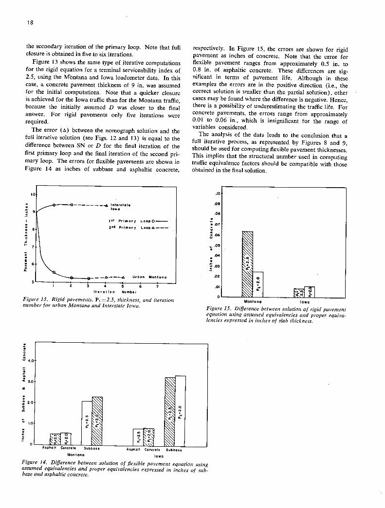
18

the secondary iteration of the primary loop. Note that full closure is obtained in five to six iterations.

Figure 13 shows the same type of iterative computations for the rigid equation for a terminal serviceability index of 2.5, using the Mbntana and Iowa loadometer data. In this case, a concrete pavement thickness of 9 in. was assumed for the initial computations. Note that a quicker closure is achieved for the Iowa traffic than for the Montana traffic, because the initially assumed D was closer to the final answer. For rigid pavements only five iterations were required.

The error () between the nomograph solution and the full iterative solution (see Figs. 12 and 13) is equal to the difference between SN or D for the final iteration of the first primary loop and the final iteration of the second pri-mary loop. The errors for flexible pavements are shown in Figure 14 as inches of subbase and asphaltic concrete,

10.

-------- _______- Interstate low a

let Primary LoopO-

2nd Primary Loop A----

0

a. Urban Montana

I 2 3 4 5

Iteration Number

Figure 13. Rigid pavements. P = 2.5, thickness, and iteration number for urban Montana and Interstate Iowa.

respectively. In Figure 15, the errors are shown for rigid pavement as inches of concrete. Note that the error for flexible pavement ranges from approximately 0.5 in. to 0.8 in. of asphaltic concrete. These differences are sig-nificant in terms of pavement life. Although in these examples the errors are in the positive direction (i.e., the correct solution is smaller than the partial solution), other cases may be found where the difference is negative. Hence, there is a possibility of underestimating the traffic life. For concrete pavements, the errors range from approximately 0.01 to 0.06 in., which is insignificant for the range of variables considered.

The analysis of the data leads to the conclusion that a full iterative process, as represented by Figures 8 and 9, should be used for computing flexible pavement thicknesses. This implies that the structural number used in computing traffic equivalence factors should be compatible with those obtained in the final solution.

.09

.00

.07

C 0.06

.05

.04

N .03

.02

.01

Montana Iowa

Figure 15. Difierence between solution of rigid pavement equation using assumed equivalencies and proper equiva-lencies expressed in inches of slab thickness.

4.0

3.0

2.0 -

1.0

0inT r I Asphalt concrete Subbase

Montana Iowa

Figure 14. Diflerence between solution of flexible pavement equation using assumed equivalencies and proper equivalencies expressed in inches of sub-base and asphaltic concrete.

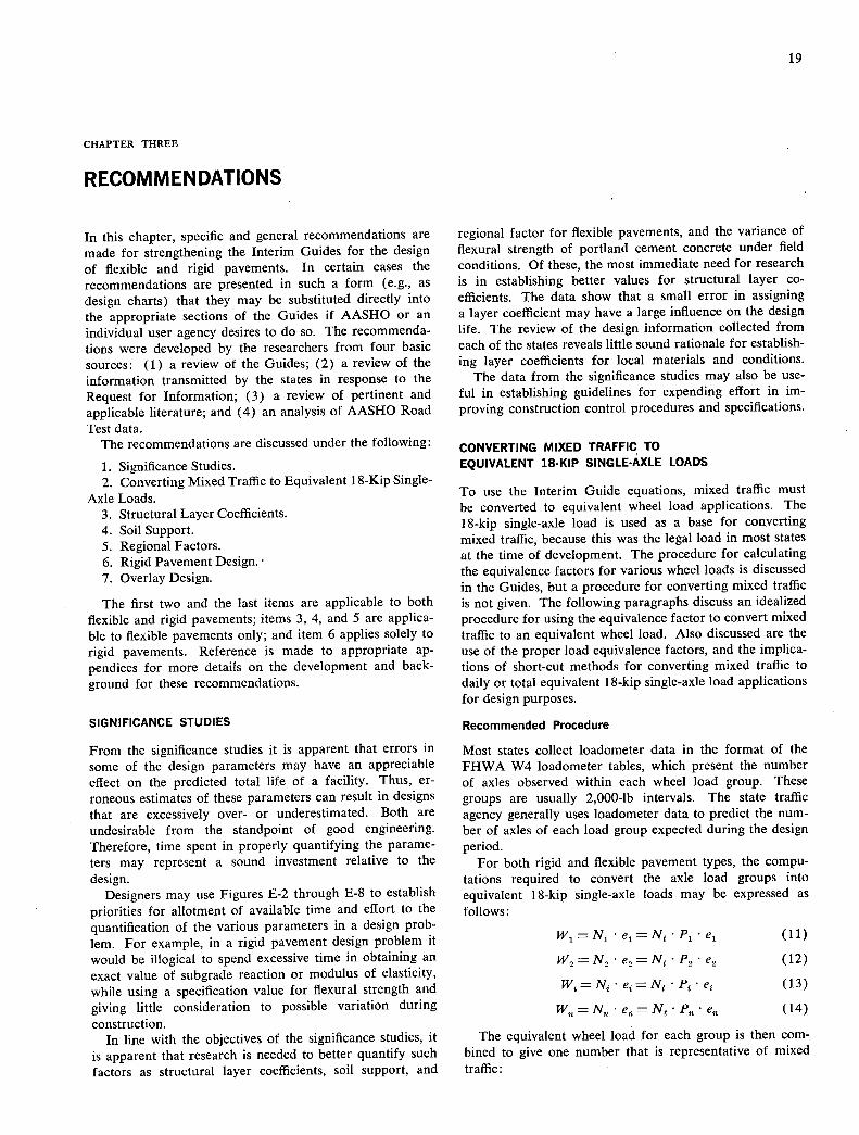
CHAPTER THREE

19

RECOMMENDATIONS

In this chapter, specific and general recommendations are made for strengthening the Interim Guides for the design of flexible and rigid pavements. In certain cases the recommendations are presented in such a form (e.g., as design charts) that they may be substituted directly into the appropriate sections of the Guides if AASHO or an individual user agency desires to do so. The recommenda-tions were developed by the researchers from four basic sources: (1) a review of the Guides; (2) a review of the information transmitted by the states in response to the Request for Information; (3) a review of pertinent and applicable literature; and (4) an analysis of AASHO Road Test data.

The recommendations are discussed under the following:

Significance Studies. Converting Mixed Traffic to Equivalent 1 8-Kip Single-

Axle Loads. Structural Layer Coefficients. Soil Support. Regional Factors. Rigid Pavement Design. Overlay Design.

The first two and the last items are applicable to both flexible and rigid pavements; items 3, 4, and 5 are applica-ble to flexible pavements only; and item 6 applies solely to rigid pavements. Reference is made to appropriate ap-pendices for more details on the development and back-ground for these recommendations.

SIGNIFICANCE STUDIES

From the significance studies it is apparent that errors in some of the design parameters may have an appreciable effect on the predicted total life of a facility. Thus, er-roneous estimates of these parameters can result in designs that are excessively over- or underestimated. Both are undesirable from the standpoint of good engineering. Therefore, time spent in properly quantifying the parame-ters may represent a sound investment relative to the design.

Designers may use Figures E-2 through E-8 to establish priorities for allotment of available time and effort to the quantification of the various parameters in a design prob-lem. For example, in a rigid pavement design problem it would be illogical to spend excessive time in obtaining an exact value of subgrade reaction or modulus of elasticity, while using a specification value for flexural strength and giving little consideration to possible variation during construction.

In line with the objectives of the significance studies, it is apparent that research is needed to better quantify such factors as structural layer coefficients, soil support, and

regional factor for flexible pavements, and the variance of flexural strength of portland cement concrete under field conditions. Of these, the most immediate need for research is in establishing better values for structural layer co-efficients. The data show that a small error in assigning a layer coefficient may have a large influence on the design life. The review of the design information collected from each of the states reveals little sound rationale for establish-ing layer coefficients for local materials and conditions.

The data from the significance studies may also be use-ful in establishing guidelines for expending effort in im-proving construction control procedures and specifications.

CONVERTING MIXED TRAFFIC TO

EQUIVALENT 18-KIP SINGLE-AXLE LOADS

To use the Interim Guide equations, mixed traffic must be converted to equivalent wheel load applications. The 18-kip single-axle load is used as a base for converting mixed traffic, because this was the legal load in most states at the time of development. The procedure for calculating the equivalence factors for various wheel loads is discussed in the Guides, but a procedure for converting mixed traffic is not given. The following paragraphs discuss an idealized procedure for using the equivalence factor to convert mixed traffic to an equivalent wheel load. Also discussed are the use of the proper load equivalence factors, and the implica-tions of short-cut methods for converting mixed traffic to daily or total equivalent 18-kip single-axle load applications for design purposes.

Recommended Procedure

Most states collect loadometer data in the format of the FHWA W4 loadometer tables, which present the number of axles observed within each wheel load group. These groups are usually 2,000-lb intervals. The state traffic agency generally uses loadometer data to predict the num-ber of axles of each load group expected during the design period.

For both rigid and flexible pavement types, the compu-tations required to convert the axle load groups into equivalent 18-kip single-axle loads may be expressed as follows:

W1 = N1 e1 = N - P1 - e (11)

W,=N9e2NP9e2 (12)

W j Ni - ei = Nt Pi e (13)

13' = N e =Nt P,,e (14)

The equivalent wheel load for each group is then com-bined to give one number that is representative of mixed traffic:

20

W 18 = W1 + W2 . + W . + W, (15a)

Wt18=, = lu (15b)

or

N °' = ("t) ('i) ( 15c)

in which

W 8 = total equivalent 18,000-lb single-axle loads due to mixed traffic;

Ni = number of axles expected for a given load group; Nt = total number of axles expected; P4 = percentage of axles in any given load group; and e4 = traffic equivalence factor for a given axle group

and pavement type.

The formula for computing the 18-kip traffic equivalence factor for flexible pavements that encompasses all the design parameters is:

ei = W1

1(18 (Li + n) 479 10°/a ' _____ w, + 1)4.79][l0G/)(fl4.33) (16)

in which

n = designation of axle type (i.e., n = 1 for single axles and n = 2 for tandem axles); and

Li = average axle load for a given axle load group and type.

By substituting Eq. 16 into Eq. 15c, a general equation is obtained for converting mixed traffic to total equivalent 18-kip single-axle loads for flexible pavements:

- __________ (L + n) 479 (lOG/fl) 1.336 X 10° ' (n 33) (10°/$) (1 )

Using the same approach as above, a general equation may also be obtained for rigid pavements:

e- = w 18r (L + n) 462 ir 10fl w, [(18 + l)462][ (10°/fl) (fl4.28)] (18)

Substituting Eq. 18 into Eq. 15c:

w - N 5 'ci (L+n)°2 (10°/fl)

518 - 8.093 X lo5Zill =l (n38 ) ( 10°/fl) (19)

If design nomographs are developed for solving the thickness equations, it is recommended that the traffic scale be in terms of total traffic derived from Eqs. 17 and 19 rather than on an average daily basis. Because total traffic number is used in the equation, the design traffic is inde-pendent of design life in the nomograph, and one chart may be used regardless of the period selected for design. This also allows consideration of stage construction.

Lane and Directional Distribution

The equivalent wheel loads derived from the foregoing procedure represent the totals for all lanes in both direc-tions. This traffic must be distributed by lanes for design purposes. A review of the highway agency design manuals revealed no criteria for directional distribution. Most states

use a 50/50 directional split, with a note that special conditions may warrant some other split.

With regard to lane distribution, most states assign 100 percent of the traffic in a given direction to the design lane. Other states have developed lane distribution factors for multilane facilities. Table 3 gives the range of distribu-tions for various numbers of lanes used by the highway departments. * If there is doubt as to what factor to apply, it is suggested that the upper side of the range be used in design.

Use of Proper Traffic Equivalence Factors

Eqs. 16 and 18 indicate that the traffic equivalence fac-tors are a function of the expected terminal serviceability (Pt) and pavement structure dimensions, as well as the axle load. In Appendices A and B of the AASHO Interim Guide for Design of Pavement Structures (86), detailed tables give the traffic equivalence factors for various struc-tural numbers and terminal serviceability values.

A review of the information received from the states indicates that most states have adopted traffic equivalence factors obtained from weighted averages of the various structural numbers or pavement thicknesses for a given axle load. In sornc cacs the tiaffie data available may not justify the use of the more accurate computations, but, in any case, the possible error resulting from the short-cut approach should be realized. For both pavement types, the equivalence factors for the upper and lower ranges of thick-nesses are approximately equal, but there is a considerable difference between the extreme ranges and the middle range of pavement thicknesses. For flexible pavements, the equivalence factors between a structural number of 1 and 3 may vary as much as 20 percent for the heavier axle loads and up to 50 percent for the lower axle loads. Varia-tion may also be noted in terms of the terminal service-ability index, with up to 20 percent variation in the equivalence factors for both the upper and lower ranges of wheel loads.

The meaning of the axle load equivalence is more readily understood if applied to actual loadometer data. Using a traffic equivalence factor for the average axle load of each load group for a typical highway (Table C-i), the numbers were converted to the average daily equiva-lent 18-kip single-axle load applications for various as-sumed structural numbers and terminal serviceability as given in Table 4. The difference in equivalent wheel loads for the various structural numbers may be interpreted as a difference in predicted pavement life. For example, if a structural number 3 is used to compute the equivalencies, and the final design is a structural number 1, the design life could be up to 4 percent less than anticipated.

The complete equations (i.e., Eqs. 16 and 18) should be used for computing the traffic equivalence factors. Short-

* Information from Arizona, California, Georgia, Illinois, North Caro-lina, Pennsylvania, and Texas used in developing the table.

21

cut procedures that do not take into account the total performance equation may result in substantial errors in computing the equivalent axle loads. For example, sim-plified versions of Eqs. 16 and 18 may be developed by making a log-log correlation between the 18-kip single-axle load and axle load being considered of the following form:

e = (L/L) 11 (20)

in which

L = the axle load being considered;

L = the axle load being used as a basis for equating other axle loads (i.e., 18-kip single-axle load); and

n = slope of correlation line.

A correlation may be obtained with Eq. 20 for fixed values of such factors as pavement thickness and terminal serviceability, but a change in a factor requires a new correlation.

Evaluation of Current Methods

In Appendix C, some of the methods used by the state highway agencies for converting loadometer data to equiva-lent 18-kip single-axle load applications are discussed. Method A is represented by Eqs. 17 and 19, and is the procedure for converting mixed traffic that will give the greatest accuracy in predicting the equivalent axle loads from the loadometer data as they are presently collected. Therefore, this method is used as a basis for comparing the accuracy of the other methods under various wheel load distributions and traffic.

Description of Current Methods

Following are brief descriptions of each of six other meth-ods currently used for determining traffic equivalence fac-tors. In Appendix C these procedures and their limitations are discussed in more detail.

Method B—Based on classifying vehicles into three broad types: passenger cars, single-unit vehicles, and multi-unit vehicles. A weighted traffic equivalence factor for each such vehicle type, based on the statewide average for various roadway classifications, is used to convert to equiva-lent 18-kip single-axle loads. The equivalent 18-kip single-axle load applications for each vehicle type are then distributed to the design lane.

Method C—Similar to Method A, except that only 10 axle groups are used, instead of the 24 or more groups that may be used with Method A. An estimate is made of the total number of axles expected to use the facility in the future. Then, an estimate is made of axle distributions, and weighted traffic equivalence factors are applied to arrive at a figure for total equivalent 18-kip single-axle loads.

Method D—Similar to Methods A and C, except that the technique used to predict increase in traffic takes into account a possible significant change in distribution of axle loads in the future. This concept could be particularly valuable for states experiencing a rapid growth in traffic, because a shift in distribution often accompanies such growth.

TABLE 3

LANE DISTRIBUTION FACTORS ON MULTILANE ROADS

NO. OF LANES PERCENT OF LOADS

IN EACH DIRECTION IN DESIGN LANE

1 100 2 80-100 3 60-80

TABLE 4

COMPARISON OF DAILY TRAFFIC FOR A MARYLAND LOADOMETER STATION USING TRAFFIC EQUIVALENCE FACTORS FOR DIFFERENT ASSUMED STRUCTURAL NUMBERS AND TERMINAL SERVICEABILITY INDEX VALUES a

Pt SN=l SN=3 SN=6

2.0 1645 1626 1624 2.5 1645 1620 1587

a Numbers in table are the daily equivalent 18-kip single-axle load ap-plications, derived from the loadometer data. pe = terminal serviceability index.

Method E—Basic features are the use of heavy com-mercial ADT as a base for conversion to equivalent 18-kip single-axle loads, and an evaluation of seasonal variations in traffic. The method was developed for one of the north-ern states that experiences considerable seasonal variation in the type and distribution of axle loads.

Method F—Basic precept is that all vehicles are classified by axle type, and each vehicle type is represented by an average traffic equivalence factor. The present num-ber of average daily trucks for each axle type is multi-plied by an expansion factor for the type, based on assumed growth trends. The product gives the expanded average daily truck traffic expected at the end of ten years. This figure is. then multiplied by an equivalence factor for each of the axle types to obtain the average annual equivalent 18-kip single-axle load applications per axle type. The summation of these is the total average annual equivalent 18-kip single-axle load applications for use in design.

Method G—The same as method F, except that Eq. 20, instead of Eq. 16 or 18, is used to convert the total of traffic equivalence factors from a lO-kip axle-load basis to an 18-kip single-axle basis.

Evaluation of Methods

Method A is used as a basis for making this evaluation, because it represents the most detailed and accurate method of converting mixed traffic to equivalent 18-kip single-axle load applications using the type of loadometer data pres-ently available. The variation in the total equivalent 18-kip single-axle load applications computed by the various meth-ods may be taken as a measure of the variation expected in pavement life, assuming that the same design method is

22

used with the equivalent axle loads. The variations may also be presented in terms of surface or subbase thickness differences as determined by the Interim Guide equations.

For the purpose of comparison, data from three load-ometer stations in various areas of the U.S. were selected for analysis by each of the methods. Two Interstate high-ways, one in Ohio and one in Iowa, were selected to show the effect of traffic distribution. The third loadometer sta-tion, an urban location in Montana, shows the effect of highway type as well as of geographical area. Data for each loadometer station and the assumptions pertaining to the extension of these data are given in Appendix C (Table C-7).

The data for each loadometer station were converted to total 18-kip single-axle load applications by each of the methods. Tables 5 and 6 give the percent deviation in W, from that obtained with Method A, with a positive sign indicating a larger value, and a negative sign a smaller. The percentages in Tables 5 and 6 may be used directly to compute the error in predicted life. For example, if a value of -20 percent is obtained, it may be assumed that a road designed to last 20 years may last only 16 years. The larg-est error (+241 percent) is with the Montana loadometer station using Method B, which means the life would be approximately 21/2 times as long as intended. The most critical errors are with Method F, where differences greater than -50 percent are obtained. This difference may be interpreted to mean that the roadway may last only 10 years when designed to last for 20 years. Method C generally gives the least error.

The large variation in the computed total equivalent 18-kip single-axle load applications with each of the meth-ods may be partially explained by the axle load distribution for each of the loadometer stations considered (see Ap-pendix Q. The Montana loadometer station data have almost no tandem axles and 93 percent of the axles are less than 5 kips. In contrast, the Iowa data show about 47 per-cent tandem axles, as well as 2 percent of the single axles over the 18-kip limit and 6 percent of the tandem axles over the 32-kip limit. These two loadometer stations prob-ably represent extremes in variation from the statewide averages used in deriving Methods B through E. If these

distributions had by chance been close to the statewide averages, the differences given in Tables 5 and 6 would have been small.

The total equivalent 18-kip single-axle loads were con-verted to pavement thicknesses by Eqs. 6 and 9. Some of the results are shown in Figures 16 and 17. These figures show the difference between the thickness obtained using Method A and the method indicated. For flexible pave-ments, the difference in structural number has been con-verted to inches of asphaltic concrete surfacing, using the coefficient of 0.44 developed in the AASHO Road Test conditions.

Summary

The data presented show that errors may result from taking short-cut steps in converting mixed traffic. This means that the life of a roadway could be underestimated or over-estimated, depending on the means used to convert to mixed traffic. These errors are in no way related to the method of predicting future traffic, which may be a further source of error.

The foregoing statements do not necessarily mean that a state highway department using one of the foregoing methods that they have developed is seriously under-designing their pavements, because their design procedure (including selection of soil support and regional factor) probably compensates for this error. The real danger comes when another agency adopts one of the methods for use with its own design methods or the Interim Guide, in which case serious errors may result.

On the basis of this study, it is strongly recommended that mixed traffic be converted to equivalent 18-kip single-axle loads by use of Method A (i.e., Eqs. 17 and 19). The fact that traffic projection is not an exact science does not justify taking short-cut procedures that may result in com-putation errors. To minimize these errors, the calculation method giving the most accurate results from available data should be used.

STRUCTURAL LAYER COEFFICIENTS

One of the limitations of the Interim Guide for flexible pavements is that no guidance was given for selecting struc-

TABLE 5

PERCENT DEVIATION FROM METHOD A TABLE 6

BY VARIOUS METHODS OF CONVERTING TRAFFIC PERCENT DEVIATION FROM METHOD A BY (FLEXIBLE PAVEMENT) VARIOUS METHODS OF CONVERTING TRAFFIC

(RIGID PAVEMENT) PERCENT DEVIATION, BY LOCATION AT LOADOMETER STATION PERCENT DEVIATION, BY LOCATION AT

METHOD OF URBAN, INTERSTATE, INTERSTATE, LOADOMETER STATION

CONVERSION MONTANA OHIO IOWA METHOD OF URBAN, INTERSTATE, INTERSTATE,

B +127.6 -33.1 -36.6 CONVERSION MONTANA OHIO IOWA

C -14.6 -15.8 +26.0 B +240.8 +8.4 -18.9 D +15.9 -4.1 +10.0 C +16.4 +8.4 +11.1 E +65.5 -51.7 -52.4 E +183.4 -37.0 -30.5 F -50.6 -64.1 -55.9 F -35.5 -66.5 -53.9 G -30.0 -49.2 -37.6 G -9.0 -52.5 -34.7

1 1 2 112 l'z D E F

'2 B

23

Where Pt2.5

Where Pt2.0

2 Urban Montana pcc Interstate Ohio

ACP

Figure 16. Comparison of difference in various methods of converting mixed traffic in terms of asphaltic concrete thickness and portland cement concrete, Interstate Ohio and urban Montana loadoineter stations.

Where Pt2.5

Where Pt'Z.O 1.0

I • Interstate lowo

2-Interstate Ohio

1.0

H

V-i

2.0 I I

i1 112 12 112 112

Figure 17. Comparison of difference of methods of converting mixed traffic in terms of portland cement concrete thickness, Interstate iowa and Interstate Ohio loadometer stations.

tural coefficients for materials different from the AASHO Road Test. In this section, layered elastic theory is used to develop a rational method for selecting structural layer coefficients. Included are brief discussions on the theo-retical background; on the effect of elastic properties and dimensions on coefficients; and on guidelines for selecting layer coefficients.

Theoretical Approach

Several investigators [including Skok and Finn (64), Dor-

mon and Metcalf (65), Monismith, et al. (66), and Coff-

man, et al. (67)] have previously attempted to use layered elastic theory to determine the effect of different material properties on such indices of performances as deflection and vertical stress or strain on the subgrade. Coffman, et al. (67) made a significant contribution in determining

variations in the relative effectiveness of different paving materials. Using layered elastic theory, Coffman deter-mined variations in layer equivalencies (the thickness of material in one layer equivalent to 1-in, thickness of another material) between asphaltic concrete surfacing and asphalt base with time of day and as a function of time of year. Coffman concluded that ". . . there is no unique equivalence and that the inclusion of a failure term is necessary to the theoretical calculation of equivalence for given materials, environment, and loading." As a result of these investigations, it was decided that layered elastic theory could be used as a first step in determining varia-tions of structural layer coefficients under different loading, environmental, and structural conditions.

On the basis of a detailed search of the literature per-taining to studies of Road Test materials (64, 68, 70, 72), the elastic properties shown in Figure 18 were assigned to

24

each layer. The background material for these selections appears in Appendix C.

Figure 18 also indicates the loading conditions assumed for purposes of this analysis. The response of the pavement to an I 8-kip single-axle load (a 9-kip dual-tire load) is used for this analysis. It is recognized that the coefficients may vary with magnitude of the load, but, in order to develop a conceptual approach, only the 18-kip axle load is used.

Discussion of Analysis

To establish structural layer coefficients for various condi-tions and materials, a limiting criterion at some point in the structure must be formulated to use as a basis of compari-son. For the purpose of this investigation, three different limiting criteria are used: (I) surface deflection, (2) ten-sile strain on the asphaltic concrete, and (3) vertical com-pressive strain on the subgrade. Surface deflection was selected for use in developing theoretical structural layer coefficients, because AASHO Road Test results have shown that this factor correlates well with observed performance. Tensile strain in the asphaltic concrete was selected because several investigators have shown the significance of the magnitude of tensile strain on the fatigue life of asphaltic concrete pavements. Vertical strain in the subgrade was selected because of its direct correlation with performance, particularly in terms of riding quality or, possibly, of rut depth.

Following is a discussion of the surface structural layer coefficient as a function of surface thickness, surface modu- lus, subgrade modulus, and base modulus. The discussion is confined to the surface layer and limiting criteria based on subgrade strain, in order to emphasize the many factors influencing layer coefficients. These few examples serve to illustrate the fallacy of using a single coefficient for a given material for all environmental and geometric conditions. For additional information see Appendix C.

Figures 19 and 20 show the variation in structural layer coefficients of asphaltic concrete as a function of thickness. Figure 19 is for a summer condition, and Figure 20 is for

4500 lbs. 4500 lbs.

150,000 psi —Summer ASPHALT I CONCRETE

D1 'Var. E1 • 600,000 psi—Fall S Spring

900,000 psi - Winter

AGGREGATE

BASE 02 'Var. E2 15,000 psi

I, 30,000 psi

3,000 psi

SUBORADE 03 00 E3 • 7,000 psi

15,000 psi

a spring condition. In both cases, the variation is for a subgrade, modulus of 3,000 psi and a base modulus of 15,000 to 30,000 psi.

Note that in Figure 19, for the summer condition, the asphaltic concrete coefficient does not change significantly as the thickness of the asphaltic concrete increases. How-ever, for the spring condition, the coefficient increases as the thickness of asphaltic concrete is increased from a relatively thin section of about 3 in. to a thicker section of about 7 in.

Figure 21 shows the effect of varying subgrade modulus from 3,000 to 15,000 psi on the asphaltic concrete layer coefficients. In general, the asphaltic concrete layer co-efficient is relatively constant over the range of subgrade modular values investigated.

Figure 22 summarizes the results of layer coefficient computations for two combinations of base and surface moduli. The figure shows that for the summer modulus value for asphaltic concrete (150,000 psi) the asphaltic concrete layer coefficients are much lower than the values determined at the Road Test. For the spring surface modu-lus condition the asphaltic concrete layer coefficient in-creases with an increase in base modulus. This is attribut-able mainly to the lower deflections associated with this higher base modulus.

Guidelines for Selecting Coefficients

On the basis of the information provided by the RFI and the theoretical implications discussed in the previous sec-tion, the following guidelines for selecting structural layer coefficient are presented. It should be recognized that, throughout this discussion, the layer coefficient for crushed stone base remains constant; i.e., variations have been normalized 1 about the layer coefficient a0 = 0.14 (or E., = 30,000 psi).

Determination of Structural Layer Coefficient (a1)—Asphaltic Concrete Surfacing

Figure 23 provides a direct determination of a1 as a func-tion of selected material properties. The average value for Marshall stability on the Road Test was 2,000 lb. This value was used as a base for increasing and decreasing a1,

using information in Appendix C as a guide. The adjust-ment for Hveem cohesiometer value was made in a similar manner. The average modulus was determined from the average pavement temperature (T = 67.5 F) and data presented by Kallas and Riley (73). The adjustment in a1 was normalized about a modulus of 450,000 psi and a layer coefficient of 0.44.

Adjustments to a1

No adjustment is needed in the value a1 over the normal range of thicknesses D1 and subgrade modular values E3. There is an inherent change in layer coefficients as a func-

* Normalize refers to the reduction to a standard value for purposes of evaluation or analysis. Figure 18. Schematic of layered system and load conditions.

Note: Based on equal values for vertical compressive strain for subgrade.

AASHO ROAD TEST

1 v iO 1 ------

30,000 PSI

5,000 PSI

E1 0 150,000 PSI

03 = 3,000 PSI

0.70

z

0.56 0

.0

0.42 .0

:5

Ot 0.28

z 0

0.14

so r

so

E 2 30,000 PSI-V

AASHO ROAD TEST

E 1 n 600,000 PSI

E 3 0 3,000 PSI

Note: Based on equal values for vertical compressive strain for subgrade.

25

0.70

z

0,56 uj

2-4 4-6 6-8 8-10

D1, INCHES

Figure 19. Structural layer coefficient as a function of D1.

2-4 4-6 6-8 8-10

INCHES

Figure 20. Structural layer coefficient as a function of D,.

0.42

0.14

Once: Based on equal values foe vertical

AASHO ROAD TEST

A.C. THICKNESS, IN.

£ - 2-4

o 600,000 U - 4-6

0 15,000 S - 6-8

V - 8-10

0.70

0 '-' 0.56

.0

.0 0.42

is

0.28

z 0

0.14 C.

.0

Note: Based on equal values for vertical compressive strain for subgrade.

5S oo

5 -

S

AASHO ROAD TEST .e" VALUE FOR A.C. - -

150,000

-

INCHES

___2-4

4-6

3,000 7,500 15,000

Es, PSI

Figure 21. Asphultic concrete structural layer coefficient as a function of subgrade modulus (E1) and asphaltic concrete surfacing thickness.

15,000 E2, pi

30,000

Figure 22. Aspizailic concrete structural layer coefficient as a function of base modulus (E1), surface course modu-lus (E5), and surface course thickness (D1) when E1 =3,000 psi.

tion of base modulus E. (see Figs. 19, 20, and 22). Con-sideration should also be given to magnitude of load and number of repetitions.

Determination of Structural Layer Coefficient (a,)-Granular Material

Figure 24 provides a determination of a2 as a function of pertinent material properties. Average a2 value for the Road Test crushed stone base course was 0.14. Values for CBR and R-value of the Road Test crushed stone were assigned on the basis of test results presented by Shook and

Fang (72). These points were used as a base for increasing or decreasing a2.

Adjustment to a.,-Granular Materials

No adjustment is needed for a2 for granular material for variations in load, etc., because a2 was assumed to be con-stant for all conditions except base strength.

Determination of a,-Treated Materials

Figures 25 and 26 provide a determination of a2 for cement- and bituminous-treated bases. For cement-treated

1000

800

600

400

a, 200

8 o 53

10.0

9.0

8,0

7.0

0 6.0 -

5.0 e

0.30

.28

.26

.24

.22

0.20

.18

.16

.14

0.12

0.10

26

0.6

10.0

9.0

7.0'

6.0

5.0

2)00 45 2000 900 200 , a, ieo 0 4.0 0

04 1700

- 600

500

400 - 3.0 '

300 50 .

200 2.5

1100 125

0.3 u000

900 2•0

800 100

700 1.5

600

500

400

0.2 300

1.0 Scale derived by averaging correlations obtained from The Asphalt

Institute, Illinois, Louisiana, New Menico, and Wyoming. (2)Scale derived by averaging correlations obtained from California and Texas. 3 Scale derived on this project.

Figure 23. Variation in a1 with surface course strength parameter.

bases, use was made of existing data to vary a. with 7-day compressive strength. For bituminous-treated bases the variation in a. with Marshall stability was used. This pro-vides for an inherent decrease in the coefficient, depending on the layer's position in the structural section. The scale for modulus was developed from Figure 23 so that the Marshall stability-modulus relationship is retained.

Adjustments to a.,-Treated Materials

Appendix C provides an indication of the effect of load and repetitions on the coefficient a.,. Definite consideration should be given to use of a lower a., for bituminous-treated materials as load and repetitions increase.

Determination of Structural Layer Coefficient (a3)-Granular Materials

Figure 27 shows a determination of a3 as a function of pertinent material properties. The variation in a3 with CBR, R-value, and Texas triaxial was determined from information obtained from replies to the RFI. The varia-tion of a3 with modulus was determined from theory for the case of the modulus normalized about 15,000 psi.

0.25

0.18

0.16 .!

0.14 100 85 2.0 ° 70 E 80

0.12 60 a,

- SOW a,

40° 70 z: 2.0 0.10 30

60 > a, 0.08 a

20

0.06 50 4.0

0.04

0.02

Scale derived by averaging correlations obtained from Illinein. Scale derived by averaging correlations obtained from California.

New Mexico, and Wyoming. Scale derived by averaging correlations obtained from Texas. Scale derived on project.

Figure 24. Variation in granular coefficient (a2) with base .t, WIIX(lf purarneleis.

0 - -I- ._L.

(I) Scale derived by averaging correlations from Illisois, Louisiana. and Texas. (2)r Scale derived on this project.

Figure 25. Variation in a, for cement-treated bases with base strength parameter.

0.5

400

300

401

30 0 0

25 °

20

'5

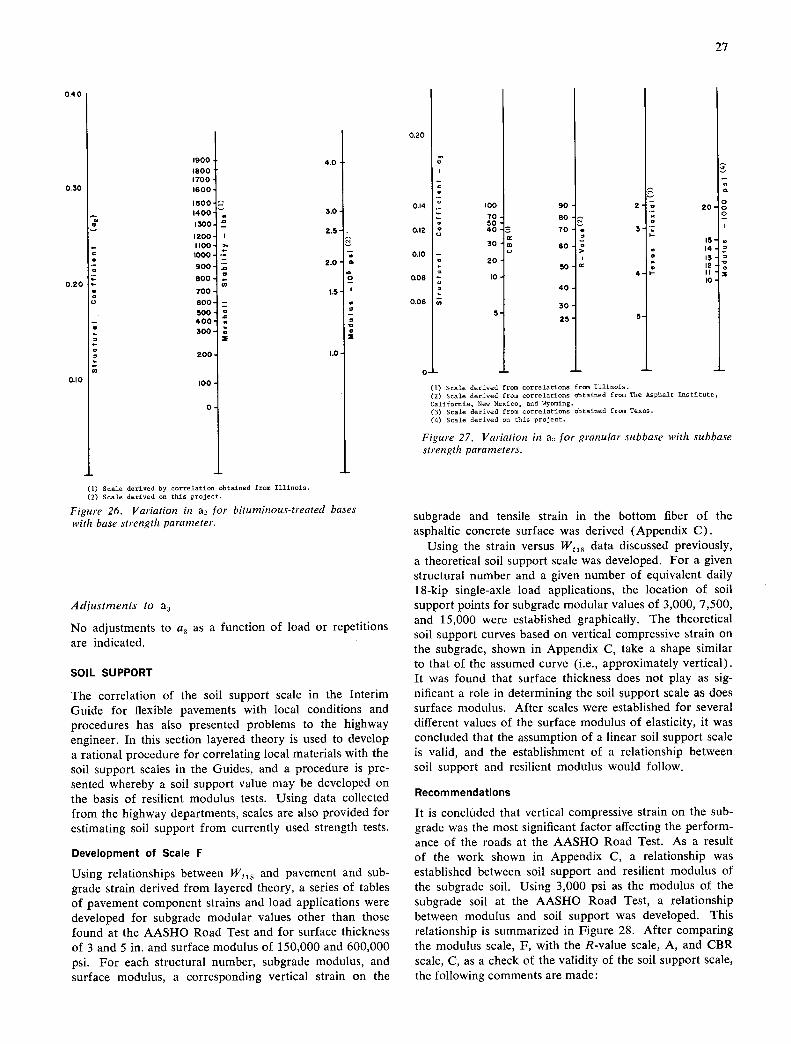
0.30

4.0

3.0

2.5 -

2.0

0

1.5

I.0

20 0 0

IS 14 = IS = 12 II I0 0.20 I

0

900

18001 1 700 600

1500 400 •

300 f 200 I 1100 1000

900

800 '5

700

600 - 500 400 300

90-1 2

80

705 C

60

50 4 -

40

30

25

0.20

0.14 . 100

70- 50-

0.12 40-

30 0.10 -

20

cfOB 10

0.06

5

0.40 I

27

Scale derived from correlations from Illinois. Scale derived from correlations obtained from The Asphalt Institute,

California, New Mexico, and Wyoming. Scale derived from correlations obtained from Tenon. Scale derived on this project.

Figure 27. Variation in a for granular subbase with subbase strength parameters.

0.10 100 -

0-

(1)Scale derived by correlation obtoimed from IJ.limnio. ( 2 ) Scale derived on this project.

Figure 26. Variation in a3 for bituminous-treated bases with base strength parameter.

Adjustments to a3

No adjustments to a3 as a function of load or repetitions are indicated.

SOIL SUPPORT

The correlation of the soil support scale in the Interim Guide for flexible pavements with local conditions and procedures has also presented problems to the highway engineer. In this section layered theory is used to develop a rational procedure for correlating local materials with the soil support scales in the Guides, and a procedure is pre-sented whereby a soil support value may be developed on the basis of resilient modulus tests. Using data collected from the highway departments, scales are also provided for estimating soil support from currently used strength tests.

Development of Scale F

Using relationships between W 1 and pavement and sub-grade strain derived from layered theory, a series of tables of pavement component strains and load applications were developed for subgrade modular values other than those found at the AASHO Road Test and for surface thickness of 3 and 5 in. and surface modulus of 150,000 and 600,000 psi. For each structural number, subgrade modulus, and surface modulus, a corresponding vertical strain on the

subgrade and tensile strain in the bottom fiber of the asphaltic concrete surface was derived (Appendix C).

Using the strain versus W558 data discussed previously, a theoretical soil support scale was developed. For a given structural number and a given number of equivalent daily 1 8-kip single-axle load applications, the location of soil support points for subgrade modular values of 3,000, 7,500, and 15,000 were established graphically. The theoretical soil support curves based on vertical compressive strain on the subgrade, shown in Appendix C, take a shape similar to that of the assumed curve (i.e., approximately vertical). It was found that surface thickness does not play as sig-nificant a role in determining the soil support scale as does surface modulus. After scales were established for several different values of the surface modulus of elasticity, it was concluded that the assumption of a linear soil support scale is valid, and the establishment of a relationship between soil support and resilient modulus would follow.

Recommendations

It is concluded that vertical compressive strain on the sub-grade was the most significant factor affecting the perform-ance of the roads at the AASHO Road Test. As a result of the work shown in Appendix C, a relationship was established between soil support and resilient modulus of the subgrade soil. Using 3,000 psi as the modulus of the subgrade soil at the AASHO Road Test, a relationship between modulus and soil support was developed. This relationship is summarized in Figure 28. After comparing the modulus scale, F, with the R-value scale, A, and CBR scale, C, as a check of the validity of the soil support scale, the following comments are made:

28

90

9-

-7—;- —50----- _j 0 -50 z ci)

4 - 4.0

—ci, 2___ -I lO___

0

40 9 — — I-.

6 - -! -i — 0

20 4 50 -10

4— 20 3

Co 0 IS

.3— 2..................

0 20

2- 0 6.0

The correlation is with the design curves used by California; AASHO desigsation is 1-173-60, and exudation pressure is 240 psi. See Hveem, P.M. and Careany, R.M .."The Factors Underlying the Rational Design of Pavements.' Proc. HOE, Vol. 28 (1948) pp. 101-136.

The correlation is with the design curves used by Waohingtoo Dept. of Highways; exudation pressure is 300 psi. See "Flexible Pavement Design Correlation Study." HRB Bull. 133 (1956).

The correlation is with the CBR design curves developed by Kentscky. See Drake. W.B. • and Bavess, J.H., "Re-Evaluation of Kentucky Flexible Pavement Design Criterion." BOB Bull. 233 (1959) pp. 33-56. The follow-ing conditions apply to the laboratory-modified CBR: specimen is to be molded at or near the optimum moiuture content as determined by AASHO T-99; dynamic compaction is to be used with a hammer weight of 10 lb dropped from a height of 18 in.; specimen is to be compacted in five equal layers with each layer receiving 10 blows; specimen is to be soaked for 4 days.

This scale has been developed by comparison between the California R-value and the Group Index determined by the procedure in Proc. gRE. Vol. 25 (1945) pp. 376-392.

Figure 28. Correlation chart for estimating soil support (S).

In available literature the modulus of a good crushed stone or aggregate base is reported to range from 15,000 to 35,000, depending on the magnitude of the vertical stresses applied. This would correspond to an R-value of the range of about 60 to 85 and a CBR of about 20 to 80. Both of these ranges are in line with what is usually considered to be the range from a good aggregate subbase to a good aggregate base. Thus, the scale F appears to be reason-able in the upper ranges.

For subgrade soils, a 3,000-psi modulus is considered to be a poor soil, whereas a 10,000-psi modulus would be considered good. When one compares these values with scales A and C, it can be seen that, for the range of modu-lar values from 31000 to 10,000 psi, the corresponding range of R-value would be from 10 to about 45, and CBR

from 2 to about 10. This indicates that the scale F appears reasonable in the lower range also.

On the basis of this investigation, it appears that the soil support scale assumed in the Interim Guide is reasonably valid. However, when R-value, CBR, and modulus as determined in this section are compared with the relation-ships between R-value, CBR, and modulus developed in the structural layer coefficient analysis, there is a slight dif-ference, particularly at the higher values of modulus. This difference is attributable to the different method of analysis. In the case of the soil support scale, the relationship be-tween soil support and modulus was determined on the basis of vertical strain in the subgrade.

REGIONAL FACTORS

The sensitivity analysis of the parameters of the design equation for flexible pavements showed that an error in selecting the regional factor can have an effect on the solution. Of the parameters considered in the flexible equa-tion, it is probably the least well defined. The results of a limited study of regional factors made in connection with this study follow. The background information for this analysis appears in Appendix C.

On the basis of information obtained from replies to the RFI, contours of equal regional factors were drawn for the United States (Fig. 29). Although these contours are only hypothetical, they do indicate agreement in regional factors between several adjacent states and lead one to believe that regional factors may ultimately be developed for all conditions.

On the basis of information presently available, it is con-cluded that the guidelines provided in the Interim Guides are still applicable for use in establishing regional factors. However, as far back as 1961, Special Report 61-E (45) pointed out the necessity for conducting satellite studies to obtain the information needed to adjust the Road Test findings to other environmental conditions and types of construction. It appears that little has been done to fur-ther the satellite study concept. If there is ever to be a rational design approach that will incorporate the effects of environment and region, it is almost imperative that a systematic program be laid out, with field test sections throughout the United States. Therefore, it is recom-mended that satellite test sections be provided throughout the United States for observation of pavement perform-ance under known traffic conditions. Preferably, these test sections should be constructed with equivalent materials and thicknesses in order to provide direct comparisons. Differences in performance at periods of time ranging from one to ten years should be noted. It would be highly desir-able if one of the series of test sections were constructed near the AASHO Road Test site.

RIGID PAVEMENT DESIGN

The revisions to the Interim Guides recommended here are primarily alterations of the existing approach to give the designer more flexibility in analysis. The information pre-sented is, in most cases, only an extension of work initiated by the AASHO Operating Subcommittee on Roadway

29

Figure 29. Contours of equal regional factors.

Design. Following are recommendations for revisions to the sections on material properties, subbase, pavement thickness, reinforcement, and load-transfer devices.

Material Properties

The review of the replies to the RFI revealed that most states using the Interim Guides have adopted the 1.33 safety factor without revision, and it is suggested that this practice be continued.

Since the Interim Guides were issued, several new types of steel have been introduced by the industry. Table 7 lists these latest types. Only the ASTM designations are given because, in some cases, the official status with regard to AASHO is unknown.

Subbase Design Chart

Because there is a current trend to use treated subbases beneath rigid pavements, the design of the subbase has become a more critical factor. A number of different cementing agents are being used, resulting in a large varia-tion of stiffness of the subbase layer. The stiffness may range from 20,000 psi for a granular material to 1,000,000 psi for a cement-stabilized granular material. The design chart for subbase should account for these differences and enable a designer to obtain a better estimate of the k-value at the top of the subbase. In order to develop criteria for such a better estimate of the k-value, linear elastic layered theory was used. For this problem, a two-layered system, similar to that shown in Figure 18, was analyzed. A 30-in.-diameter plate with an applied load of 10 psi was assumed to be placed on top of the upper layer and the resulting deflection was computed. This deflection was then divided

into the applied stress of 10 psi to obtain an estimated k-value for the layer. These computations were performed for a number of combinations of subgrade modulus, sub-base modulus, and subbase thickness. From these compu-tations a design chart was developed (Fig. 30). This chart may be compared with those currently used and presented in Appendix C.

The chart shows stiffness values with corresponding k-values of the natural subgrade material. The k-value may be obtained by procedures currently used by highway departments, or the stiffness value may be measured on samples of the material using the resilient modulus test (Appendix D). Also required with the analysis is the stiff-ness of the subbase, E, which may also be obtained by means of the resilient modulus test. Table 8 gives a range of stiffnesses for several different subbase types.

Figure 30 is used by entering with the subbase thickness on the vertical scale and projecting horizontally to the inter-section with the expected resilient modulus of the subbase. From this intersection a line is projected vertically until it intersects with the appropriate subgrade strength value. This point is then projected horizontally until it intersects with the vertical axis. The composite modulus of subgrade reaction (ks ), estimated for the top of the subbase, may be used with the pavement thickness design chart in the next section.

The design chart in Figure 30 was checked against the design charts used by the California Division of Highways and the Texas Highway Department, and they were found to have excellent correlation. Therefore, it is recommended that Figure 30 be used as a design chart for estimating composite modulus of subgrade reaction at the top of the subbase.

4 oq

A.

4

4

I

(9 c.

.4.

*Mhy be determined by means of the laboratory test method for Modulus of Resilience (H described herein.

noo S,

—11-1 .1 ~O00 n.

U 1000

800

U 0 Ia— 600 hi

00

0. > 400

300

200

100

0 ,

1. 6

10 12

30

LA®

Figure 30. Chart for esti,nating composite k-value

Pavement Thickness

The design equations in the Interim Guide for the design of rigid pavements were based on the Road Test equations, with modifications from theory, using the Spangler stress equation. In recent years several new theories have been developed, such as the finite element solution proposed by Hudson (76), or the axisymmetric solution of layered theory proposed by Duncan, et al. (77). These approaches

offer many advantages over the closed form aproaches, such as Spangler (78), Pickett (79), and Westergaard (80). Although the potentialities of these methods were fully recognized, the decision was made in this study to recommend to continue with the use of the combination of Spangler's equation and Road Test approach, for the following reasons:

The more complex theories will require considerable development work before application can be made on a nationwide basis.

Studies of soil conditions other than those at the Road Test are required.

The present approach, although subject to limitations, has proven to give reasonable solutions, and, with a few modifications, additional flexibility may be realized.

All state highway departments are presently using some modification of the Westergaard approach, and for all to change before a new procedure is perfected would be hard to justify.

This is not meant to imply that the development of new approaches should be discontinued. On the contrary, this work should be continued so that applications may be made in the near future.

In Appendix B of the AASHO Interim Guide for De-sign of Pavement Structures (86), a limited explanation of the development of the design equation is presented. Design nomographs were prepared with scales for equiva-lent 1 8-kip single-axle load applications, working stress of concrete, modulus of subgrade reaction, and slab thickness. Although included in the design equations, modulus of elasticity of the concrete and continuity of the slab were not considered design parameters in the charts. It is pro-posed that the two additional terms now be included in the design charts, and, further, that the design equation en-compass a regional factor similar to that used in the Interim Guide for flexible pavements.

One reason for the recommended inclusion of a modulus of elasticity for concrete term is that in the near future more synthetic aggregates probably will be used in concrete pavements as sources of quality natural material become more scarce. The concrete produced from synthetic aggre-gates generally has a modulus of elasticity considerably

TABLE 7

YIELD POINT STRENGTH FOR VARIOUS GRADES OF STEEL

STEEL GRADE YIELD POINT

STRENGTH (PSI)

A-496 (in fabric) 70,000 A-615, Gr. 40 40,000

Gr. 60 60,000 Gr. 75 75,000

A-15 or. M-31 Str. 33,000 Tnt. 40,000 Hard 50,000

A-431 orM-184 75,000 A-432 or M-185 60,000

TABLE 8

TYPICAL SUBBASE STIFFNESSES

STIFFNESS RANGE MATERIAL (PSI)

Granular 8,000-20,000 Cement-stabilized base 500,000-1,000,000 Cement-stabilized soil 400,000-900,000 Asphalt-treated base 350,000-1,000,000 Asphalt-emulsion-treated base 40,000-300,000

11 The resilient modulus test described in Appendix D may be used to quantify this term.

After Monismith. et al. (66) After MiIcheII (74). After Terrell (75).

31

different from that of some concrete produced with con-ventional aggregates. Thus, the design charts with a con-stant modulus of elasticity would not be applicable in many instances. The inclusion of the pavement continuity term is felt to be a necessity to provide for the several pavement types now being used; e.g., continuously reinforced con-crete pavements, and jointed pavements with a variety of load-transfer devices and systems.

The recommended rigid pavement equation is

log 0.333(4.5 - Pt) 1.624>< 10'

1+ (D+1)4

\ /D~ — 1.132\1 + (4.22_0.32Pf)[ log (215163J)(Dy 18.42)1

Z1/4

+C1Q—C2 +C3R (21)

in which the terms are as defined in the glossary, except as follows:

J = coefficient dependent on slab continuity and load conditions;

Zz Elk; E = Young's modulus of elasticity for the concrete; C1 = a constant to be analyzed;

Q = a function of the subbase quality; C. = a constant describing the quality of the Road Test

subbase; C3 = a constant to be analyzed; and R = a function of weather conditions and environment.

This equation may be presented in nomograph form for convenient use. Because few data are now available for evaluation of the regional factor term, this parameter is assumed to be equal to zero and is not considered in the analysis. It should be recognized that the nomograph solution is not a complete one and is subject to the limita-tions previously discussed. A nomograph for solving the foregoing equation for rigid pavements is shown in Fig-ure 31. The primary difference between Figure 31 and the nomographs of the AASHO Interim Guide for Design of Pavement Structures (86) is that pavement thickness may be solved in terms of six parameters instead of the three presented in the Guides. Figure 31 may be reduced to the Interim Guide format by inserting the AASHO Road Test values for pavement continuity, terminal service-ability, and modulus of elasticity of concrete.

The pavement continuity * term has been evaluated by Hudson and McCullough (8) and values of 3.2 and 2.2 were recommended for jointed and continuously reinforced concrete pavements, respectively. These values are marked on the nomograph and are suggested for use until better data become available. As a state acquires more experience regarding pavement continuity, the term may be adjusted, based on observations of deflections for the various pave-ment types under varying degrees of support and environ-mental conditions. The terminal serviceability values for

* Pavement continuity is defined as the percentage of load transferred across a pavement discontinuity, such as a joint or crack.

the class of highway being considered may also be entered on the figure. Caution is again given that the traffic equiva-lence factors used to determine the number of equivalent 18-kip single-axle load applications should be based on the terminal serviceability used in design. Attention is also called to the fact that the k-value to be used is the com-posite modulus of subgrade reaction at the top of the subbase from Figure 30. This is considered an elastic rather than a gross k-value. Work by Monismith and others has indicated that elastic deformation is of primary im-portance in pavement design. Therefore, the scale was changed from a gross k-value to an elastic k-value, using the Road Test data. The correlation between elastic k-value and gross k-value, as developed at the AASHO Road Test, is presented in Appendix C.

The concrete working stress (fe) used in the nomograph

is 0.75 times the flexural strength or modulus of rupture

(Se) as determined by AASHO Designation T-97 using third-point loading.

Reinforcement Design

The replies to the RFI indicate that if reinforcement is used, the Guides are generally used without revision. Some states have developed a standard weight of steel per square yard for a given pavement thickness, but generally these standards were also developed along the lines presented in the Guides. Therefore, the following revisions are sug-gested only for the purpose of giving more flexibility and consistency to the designer.

Attention is called to the fact that, in the Guides, the required amount of steel for continuously reinforced pave-ment is expressed as a percentage, whereas the distributed steel requirement for rigid pavements is presented in terms of area (i.e., as square inches per foot width of slab). The latter is satisfactory for estimating purposes, but is difficult to comprehend from a design standpoint. If distributed steel were expressed as a percentage, the values would be comparable with solutions obtained for continuously re-inforced concrete pavement.

Join ted Reinforced Concrete Pavement

The figure in the AASHO Interim Guide for Design of Pavement Structures (86) for distributed steel require-ments is for a fixed subbase friction factor of 1.5. This was a satisfactory assumption during the period when sand-cushion blankets were used between the pavement and the subbase; however, the current trend toward crushed stone or stabilized subbases, with a possible friction factor of 2 or more, emphasizes the need for considering the subbase friction factor as a variable in design.

A procedure for revising the formula for area of steel to express the solution in terms of a percentage 'of the cross-sectional area of the pavement is presented in Appendix C. The resulting equation is

P3 = (LFI2f)(100) (22)

in which

P8 = required steel percentage; L = length of slab between joints, feet;

log W = 7.35 log(D + 1) - 0.06 +

12

15

a

200

300

400

500

600 700 800

300

200

3

0

C

too 0 I

U

150

Figure 31. Design c/tart, alternate procedure for design of rigid pavements.

33

F = friction factor of subbase; and = allowable working stress in steel, psi.

Figure 32 is a nomograph solution of this equation. It provides much more flexibility than the one in the Interim Guides, because working stress can be varied between wide limits and the friction factor is included as a variable. The inclusion of a complete scale for working stress, in lieu of several fixed values, allows the designer to make an eco-nomic comparison of all steel types. In addition, the de-signer has the option of selecting the steel type or grade and determining the resulting required steel percentage, or

of selecting the optimum steel percentage and determining the steel type required. A critical item in the design equa-tion is the use of the appropriate friction or resistance fac-tor for the subbase material to be used. If no specific data are available, Table 9 may be used for general guidance in selecting a subbase resistance factor for design.

For two- or three-lane pavements, the practice in the past has been to use a constant transverse steel percentage across the width of the slab. An analysis of the subgrade drag theory formula that was used to derive the design equation indicates that the cross-sectional area of transverse steel may be reduced from the centerline toward the edge. On

L Pivot P5(%) f5 Line

Example Problem: L= 36 ft F = 1.9 fs=52500Psi

Answer: F 0.067%

Figure 32. Distributed steel percentage (8).

Where: Required steel percentage -

L = Width of slab—feet. F a Friction factor of subbase. f Allowable working stress in steel—psi.

(0.75 of yield strength recommended, the equivalent of safety factor of 1.33)

34

TABLE 9

SUBBASE COEFFICIENTS FOR USE IN EMPIRICAL DESIGN EQUATION

SUBBASE SUBBASE TYPE

COEFFICIENT

Surface treatment 2.2 Lime stabilization 1.8 Asphalt stabilization 1.8 Cement stabilization 1.8 River gravel 1.5 Crushed stone i.s Sandstone 1.2 Natural subgrade 0.9

These recommendations were derived from a field study reported by McCullough (81).

24-ft pavements, this is generally not a practical approach, but on multilane freeways it may be economically feasible. Figure 33 shows the design principles involved in this ap-proach. The sketch shows the influence line for the re-quired percentage of steel in terms of pavement width. The equation at the bottom of the figure may be used to com-pute the required percentage of steel at any point trans-versely across the slab. Note, for example, that if a five-module pavement is to be used, the steel required in the outer modules would be considerably less than in the interior module.

CI C2 C3 C4

I

:

+ M3 +_M4+_5

Pavement Cross Section

in which

M = concrete slab module between joints (construction or formed); X = width of concrete module; C = joint; e.g., construction or control;

= distance from a free edge to the most interior point for the area under consideration;

P9 = steel percentage required at distance .Q. from free edge; and P5 and L are as previously defined.

By definition the term 2 must Satisfy the following:

2 <

Using the influence diagram, the steel percentage required for any area may be computed as follows:

Continuously Reinforced Concrete Pavement

No change is suggested in the equation presented in the Interim Guides for determining the steel requirements for continuously reinforced concrete pavement. However, the nomograph has been revised to provide for the higher-strength steels that were not available at the time the Guides were prepared. The revised nomograph is shown in Figure 34.

Longitudinal steel should not be less than 0.4 percent for concrete made with conventional coarse aggregates, even though Figure 34 may indicate less. Deflection studies on in-service pavements have shown that the continuity con-dition across a transverse crack (full load transfer) is lost when the percentage of longitudinal steel decreases below 0.4 percent (82). In low-temperature areas, the absolute minimum should be increased to 0.5 percent. For a high-strength steel, the stresses due to volume change may be considerably less than the yield strength, but in order to develop the strength a large strain is required. This leads to excessive crack widths, and a resulting loss of load trans-fer. Some pavements with less than 0.4 percent steel have stayed in service for extended periods, but not without problems (83). In special cases, where the concrete coarse aggregate has a thermal coefficient of from 2 X 10 6 to 4 X 10- in /in /oF, the minimum allowable longitudinal steel may be reduced to 0.35 percent (85).

To permit the assumption of minimum crack widths, the ratio of the bond area of the longitudinal bars to the con-crete volume should not be less than 0.03 in.2 /in.. The bond-area ratio should be checked by the following (84):

Q=4P/D (23)

in which

Q = ratio of bond area to concrete volume, in in.2/in.3; P = steel area ratio, A 5/A,

A8 = cross-sectional area of steel, square inches per foot of slab width;

A = cross-sectional area of concrete, square inches; and D = diameter of reinforcing bars.

Steel Size and Spacing Requirements

After the required steel percentage is determined, the next design step is to determine the bar spacing and size needed to fulfill these requirements. Figure 35 is proposed for insertion into the Guides to provide the designer a simple nomograph for determining the size and spacing needed. The equation for the nomograph is

Y= (A11/DP8)(l00) (24)

in which

Y = bar or wire spacing, center to center, inches; = cross-sectional area bar wires, square inches;

D = pavement thickness, inches; and P9 = required steel percentage.

Load Transfer Devices

A review of state practice in the use of dowel bars in jointed pavement indicates that the states are essentially following

P = 2 PS

Figure 33. Procedure for designing distributed steel percentage

PS

1.0

I. I

I.0

0

o.e

0.6

0.5

0.4

0.3

F

I

1.0 1.5 to

C

Where P5 Required steel percentage-% F .Frjctjon factor of subbase S'c*Tensi$e strength of concrete- psi f5g Allowable working stress in steel-psi

(0.75 of yield strength recommended, the

equivalent of safety factor of 1.33)

SOLVES: P. (1.3-0.2F) x 100 fs

Example Problem:

Se . 300 f.45OOO F 2.0

Answer: P5:O.60

Sic

600

500 f

400 $ 52500

__.4... 45000 300 + 37500

200

tOO

Figure 34. Longitudinal steel for CRCP (8).

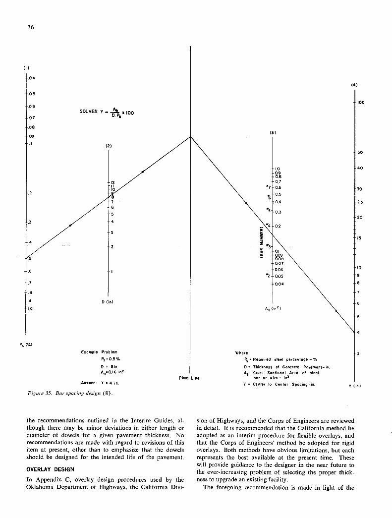
PS

100

50

40

30

25

20

5

10

9

8

7

6

5

4

3

36

answer. 1 4 In. Y Center to Center Spacing-in. y ( i,,) Figure 35. Bar spacing design (8).

the recommendations outlined in the Interim Guides, al-though there may be minor deviations in either length or diameter of dowels for a given pavement thickness. No recommendations are made with regard to revisions of this item at present, other than to emphasize that the dowels shOuld be designed for the intended life of the pavement.

OVERLAY DESIGN

In Appendix. C, overlay design procedures used by the Oklahoma Department of Highways, the California Divi-

sion of Highways, and the Corps of Engineers are reviewed in detail. It is recommended that the California method be adopted as an interim procedure for flexible overlays, and that the Corps of Engineers' method be adopted for rigid overlays. Both methods have obvious limitations, but each represents the best available at the present time. These will provide guidance to the designer in the near future to the ever-increasing problem of selecting the proper thick-ness to upgrade an existing facility.

The foregoing recommendation is made in light of the

37

fact that a number of states presently use a modification of the flexible pavement design procedure in the Interim Guides for overlay design. Such use requires the selection of a structural layer coefficient to assign to each layer of the existing pavement. This is largely a matter of judg-

ment, and is subject to considerable variation. Further-more, the procedure does not truly evaluate the load-carrying capacity of the existing pavement structure, as may be done by deflection measurements of the in-place pavement structure.

CHAPTER FOUR

CONCLUSIONS AND SUGGESTED RESEARCH

This project may be considered to be part of the continuing effort to update and improve pavement design procedures. Its basic objective is "to develop proposed revisions to the AASHO Interim Guides for the design of pavement struc-tures based on an evaluation of current state highway de-partment procedures." From the study of current highway practices, and with due consideration of recent develop-ments in analytical design theories and methods of charac-terizing properties of pavement materials, recommenda-tions were prepared for modification in a number of areas of the design procedures of the Interim Guides. The re-visions proposed are presented in the previous chapter, and satisfy the basic objective of this project. The findings re-ported herein, together with more detailed information in the Appendices, suggest the following conclusions and sug-gested research for further improvements of the Interim Guides.

CONCLUSIONS

On the basis of the findings of this investigation, the follow-ing major conclusions are drawn:

1. The Interim Guides were established on the basis of findings for one of a myriad of possible environmental, material, and construction conditions. Engineering judg-ment, together with some theoretical considerations, were used to extrapolate the results to other conditions. Un-fortunately, the relative effect of each of the variables affecting the pavement design has too often been over-looked. This study shows that:

a. Of the parameters considered in the flexible and rigid pavement equations, the SN of a flexible pavement is most significantly influenced by the structural coefficients of its various layers. The next most significant design parameter for low-traffic-volume roads (under about 100 equivalent daily 18-kip single-axle load applications) is total equivalent traffic. For high-traffic-volume roads an error in determination of soil support influences SN to a much greater extent than total equivalent traffic. The Road Test relationships indicate that

the design thickness of a rigid pavement is most significantly influenced by the fiexural strength of the portland cement concrete. The graphs herein may be used by the designer as judgment criteria for evaluating possible variability in the predicted design life in terms of the parameters used. First priority for future research toward improv-ing the Guides is to more properly quantify the structural layer coefficients for the materials used in flexible pavement construction.

2. Methods of converting mixed traffic to design traffic are numerous, and may result in differences in predicted design values. To minimize the chance for serious errors, the method giving the most accuracy with existing traffic data is suggested for immediate use. Additional conclu-sions are:

Loadometer data in the general format of the FHWA W-4 loadometer tables should be used for each axle load grouping. States experiencing growth in axle loads must project both the magnitude and the distribution of axle loads. The Load Distribution Factor (a measure of the axle-weight distribution) is an ex-cellent tool for use to keep summary statistics for given highway classifications, highways projects, or statewide averages. Because traffic is a critical factor in design, more reliable traffic data should be obtained through a wider sampling of traffic on the state highway sys-tem. The most desirable way of accomplishing this would be to install more loadometer stations for annual data collection. If this is not eco-nomically feasible, consideration should be given to increasing the number of stations and reducing the frequency of Operation. For example, little increáse in cost would result from doubling the number of loadometer stations and reducing the frequency from annually to every other year; i.e., only half the stations would be operated each year. Such a sampling at a station every two years would

38

be adequate for traffic predictions at that point, and a much broader base for projecting traffic would be available.

d. The traffic equivalence factors used for converting mixed traffic should be derived with due considera-tion of the effect of pavement thicknesses and anticipated terminal serviceability.

3. Procedures for establishing the soil support value for flexible pavement design vary from sophisticated triaxial tests to engineering judgment. For those states using the Interim Guides, the test procedures used have been cor-related with the AASHO scale through appropriate testing, or the relationships presented in the Interim Guides have been accepted. Although the original soil support scale was valid for only one point, S = 3 (or possibly two, S = 10), it was possible through theory to show the remainder of the scale to be reasonably sound. Continued effort should be made to strengthen the validity of the soil support scale as new analytical tools and methods of characterizing material properties become available.

4. Better methods are needed to establish the effects of variations in regional or environmental conditions. Exist-ing methods for establishing these effects rely almost totally on engineering judgment and on measures of critical en-vironmental parameters. Insufficient consideration has been given to differences in performance of equivalent sections under different environmental conditions. A program to systematically study these differences on a state and national basis is needed.

5. The structural layer coefficient for a given pavement material is not a constant. AASHO Road Test results showed that the structural layer coefficient of the surfacing can vary several fold, from only slightly higher than that for crushed stone base to as much as eight times higher. Although this variation in the surfacing may be attributable primarily to temperature differences, other variables that should be considered in establishing structural layer coefficients are:

The magnitude of axle loads and the number of repetitions of each. The thickness of each pavement component. The properties of the materials of each pavement component, including the subgrade. The environment, including temperature, moisture, frost, and cycles of change in each. The relative position and depth in the pavement structure.

The type of analytical studies presented herein should be continued so the behavior of pavement materials can be better understood. As new analytical tools and methods for characterizing materials become available, progress can be made toward determining coefficients for each com-ponent of a pavement for the anticipated traffic loads and environmental conditions.

6. Rigid pavements are presently designed by one of two methods: The Interim Guides or the PCA method. The recommendations in this report are aimed at improving the method presented by the Interim Guides. Recommended revisions were made in the following areas:

a. Material Properties—Because most states using the

Guides have adopted the use of concrete working stress as 0.75 times the flexural strcngth or modu-lus of rupture determined by AASHO Designation T-97 using third-point loading, it was suggested that this practice be continued. The Interim Guides should be updated to include most recent types of steel available. Subbase Design—Because of the increasing use of stabilized subbase materials, a design chart was developed to aid the pavement engineer in deter-mining support values for these materials. This chart was developed through application of lay-ered elastic theory, and was checked against cur-rent practices. Because of the excellent correlation between theory and practice, it is recommended that this chart be used for estimating the k-value for treated subbase. Thickness Design—An alternate nomograph for rigid pavement design was prepared providing for the variations in: (1) terminal serviceability in-dex, (2) pavement type (jointed or continuously reinforced), and (3) modulus of elasticity of the concrete.

Reinforcement Design—Design charts were de-veloped for determination of the percentage of steel and the size and spacing of reinforcement for reinforced and continuously reinforced con-crete pavements. For reinforced concrete pave-ments, the new chart provides additional design flexibility by including a wider range in working stress for the steel. For continuously reinforced concrete pavements, the design for percentage of steel in the Interim Guides has been revised to provide for the higher-strength steels not available at the time the Guides were prepared.

7. The review of current overlay design practices indi-cates that the few design methods available account for wheel load stresses only, with no consideration of stresses resulting from volume changes. Of the procedures avail-able, only those using deflection measurements evaluate the load-carrying capacity of the in-place pavement.

The flexible pavement design portion of the Interim Guides has been used in the design of overlays, but such an application is an extension of the empirical relationships beyond their limits. This is especially true with regard to its use with rigid pavements, because there is no basis in AASHO Road Test results for the assignment of structural layer coefficients to portland cement concrete. Therefore, a more rational overlay design procedure is needed in order to account for both wheel load and volume change stresses. Several design factors should be considered in a systems framework, such as that proposed in the report for NCHRP Project 1-10 (49).

RECOMMENDED FUTURE RESEARCH

It is strongly recommended that research be continued along the lines explored in this project. Specifically, addi-tional research is needed in the following areas:

39

Development of improved traffic projection methods to consider changes in both traffic volume and axle loads distribution. This is particularly important when looking ahead to potential increases in maximum allowable axle loadings.

Continued study to improve the soil support scale for flexible pavement design. Based on the concepts presented here, together with new analytical tools, methods of characterizing paving materials, or results of satellite stud-ies, further analyses can be made that will strengthen the base for the soil support scale.

Strengthening the basis for establishment of the struc-tural layer coefficients for each flexible pavement compo-nent. Some immediate results could be obtained if states were to begin to compare the coefficients they have used in design with performance of pavements. Long-range efforts should be directed toward developing weighted co-efficients that would be functions of traffic, thickness, and stress deformation properties of each pavement layer and of the environment.

Establishing criteria for selection of applicable re-gional factors. One approach to establishing such criteria

would be the construction of satellite test sections through-out the United States, and to observe pavement perform-ance under known traffic conditions. To be most effective, widely separated test sections should be constructed with equivalent materials and thicknesses in order to provide direct comparisons, and differences in performances at periods ranging from one to ten or more years should be noted.

Development of a more rational procedure for de-signed rehabilitation of existing pavements. Such a pro-cedure should incorporate some measure of the load-carrying capacity of the existing pavement, and should be applicable to determining overlay requirements for both flexible and rigid pavements.

Finally, it is recommended that consideration be given to further application of the systems engineering approach to the design of pavement structures, such as that de-veloped in NCHRP Project 1-10 (49). This would per-mit states to consider all aspects of pavement design dis-cussed in this report, as well as other complicating fac-tors such as economics and construction methods and techniques.

REFERENCES

"The AASHO Road Test-Proceedings of a Confer-ence held May 16-18, 1962, St. Louis, Mo." HRB

Spec. Rep. 73 (1962). "AASHO Interim Guide for Design of Flexible Pave-ment Structures." AASHO Comm. on Design (Oct. 1961) mimeo. "AASHO Interim Guide for Design of Rigid Pave-ment Structures." AASHO Comm. on Design (Apr.

1962) mimeo. TRICK, P. E., "An Introduction to Guidelines for Satel-lite Studies of Pavement Performance." NCHRP Re-

port2 (1964). TRICK, P. E., and HUDSON, W. R., "Guidelines for Satellite Studies of Pavement Performance." NCHRP

Report2A (1964). HUFF, T. S., "Satellite Studies on Pavement Perform-ance." Presented at 1965 Annual Meeting of AASHO, New York, N.Y. (1965). CHASTAIN, W. E., SR., "Application of Road Test Formulas in Structural Design of Pavement." HRB

Spec. Rep. 73 (1962) pp. 299-3 13. HUDSON, W. R., and MCCULLOUGH, B. F., "An Ex-tension of Rigid Pavement Design Methods." Hwy.

Res. Record No. 60 (1963) pp. 1-14. CHASTAIN, W. E., SR., and SCHWARTZ, D. R., "AASHO Road Test Equations Applied to the Design of Bitumi-nous Pavements in Illinois." Hwy. Res. Record No. 90

(1965) pp. 3-25.

CHASTAIN, W. E., SR., BEANBLOSSOM, J. A., and CHASTAIN, W. E., J., "AASHO Road Test Equations Applied to the Design of Portland Cement Concrete Pavements in Illinois." Hwy. Res. Record No. 90

(1965) pp. 26-41. RAND, D., and FRENCH, R., "Bituminous Concrete Pavement Inventory in Maine Correlated to AASHO

Road Test Results." Proc. AAPT, Vol. 34 (1965)

pp. 309-351. MURRAY, L. T., "Flexible Design and Experimentation in Missouri." Proc. AAPT, Vol. 34 (1965) pp. 496-

517. SKOK, E. L., JR., and DIETHELM, P. J., "Application of AASHO Road Test Results to Design of Flexible

Pavements in Minnesota." Proc. AAPT, Vol. 35

(1966) pp. 207-234. HVEEM, F. N., and SHERMAN, G. B., "Thickness of Flexible Pavements by the California Formula Com-pared to AASHO Road Test Data." Hwy. Res. Rec-

ordNo. 13 (1963) pp. 142-166.

HICKS, L. D., Discussion. Proc. International Con!.

on the Structural Design of Asphalt Pavements, Univ.

of Michigan (1962) p. 763. YODER, E. J., and MILHOUS, R. T., "Comparison of Different Methods of Measuring Pavement Condition -Interim Report." NCHRP Report 7 (1964).

40

VEsIc, A. S., and DOMASCI-IUK, L., "Theoretical Analysis of Structural Behavior of Road Test Flexible Pavements." NCHRP Report 10(1964). ISADA, N. M., "Detecting Variations in Load-Carrying Capacity of Flexible Pavements." NCHRP Report 21 (1966). KONDNER, R. L., and KRIZEK, R. J., "Factors Influenc-ing Flexible Pavement Performance." NCHRP Re-port 22 (1966). HARR, M. E., and HEAD, W. J., "Extension of AASHO Road Test Performance Concepts." NCHRP Report 30(1966). KARRH, J. B., and STEPHENSON, H. V., "Application of AASHO Road Test Results to Alabama Condi-tions." HPR Report No. 22, Alabama Hwy. Dept. (Aug. 1967). ALLEN, G. J., "New Developments in the Design of Flexible Pavements." Presented at Annual Meeting, ASCE, Arizona Section, Phoenix (Oct. 5, 1963). "Flexible Pavement Design Manual." Research Bul-letin 22-B, Florida State Road Dept. (July 20, 1960). SOWERS, G. F., "Stress, Bearing Capacity, and Flexi-ble Pavement Thickness Design Based on the AASHO Road Test and Georgia Pavement Evaluation Tests." Engineering Experiment Station, Georgia Institute of Technology, Atlanta (Feb. 1964). ERICKSON, L. F., "An Evaluation of Flexible Pave-ment Design Methods." Research Div., idaho Dept. of Highways (May 1964). DRAKE, W. B., and HAVENS, J. H., "Kentucky Flexi-ble Pavement Design Studies." Univ. of Kentucky, Engineering Res. Bull. No. 52 (June 1959). ROLAND, H. L., JR., "Texas Triaxial R-Value Correla-tion." Final Report, Research Project 61-15, HPR 1(1), Testing and Research Section, Louisiana Dept. of Highways (March 1963). "Flexible Pavement Design Standards." Bureau of Materials and Research, State Road Commission of Maryland (Revised Jan. 1, 1965). TONS, E., CHAMBERS, R. E., and KAMIN, M. A., "Layered Pavement Design Method for Massachus-setts." Hwy. Res. Record No. 71 (1965) pp. 193-219. SKOK, E. L., and RooT, R. E., "Application of AASHO Road Test Results to Design of Flexible Pavements in Minnesota." Dept. of Civil Engineering, Univ. of Minnesota (March 1967). "Structural Design Guide for Flexible Pavements." Bull. No. 102, New Mexico Hwy. Dept. (Aug. 1965). "Procedure Guide for Pavement Thickness Design." State of Oklahoma Dept. of Highways (Revised July 1965).

Pavement Design Manual. Chap. 14, "Pavement De-sign Analysis and Type Determination Method and Procedure," Penn. Dept. of Highways. "Simplified Procedure for the Design of Rigid Pave-ments." Dept. of Public Works, Commonwealth of Puerto Rico. (Revised 1967).

"Simplified Procedure for the Design of Flexible Pave-ments." •Dept. of Public Works, Commonwealth of Puerto Rico (1961).

CHU, T. Y., and HUMPI-IRIES, W. K., "The Applica-tion and Refinement of Triaxial Tests on Subgrade Materials for the Design of Flexible Pavement Struc-tures." Univ. of South Carolina (1965). "Thickness Design for Concrete Pavements." Con-crete Information, HB 35, Portland Cement Associa-tion (1966). "Flexible Pavement Design Procedure." Nebraska State Highway Dept. Manual of Instruction. Part 8, "Materials," Utah State Dept. of Highways. "Evaluation of Pavement Serviceability on Utah High-ways." Utah State Dept. of Highways (1966). VASWANJ, N. K., "AASHO Road Test Findings Ap-plied to Flexible Pavements in Virginia." Virginia Highway Research Council (1967). SCHNORMEIER, R. H., "Design of Flexible and Rigid Pavement Structures." Wyoming State Highway Dept. (Feb. 1968). HARTRONFT, B. C., "Overlays for Flexible Pavements for the 1968 Interstate Estimates." Hwy. Res. Record No. 254 (1968) pp. 68-74. ZUBE, E., and FORSYTHE, R., "Flexible Pavement Maintenance Requirements as Determined by Deflec-tion Measurement." Hwy. Res. Record No. 129 (1966) pp. 60-75. "The AASHO Road Test-Report 5, Pavement Re-search." HRB Spec. Rep. 61-E (1962). CAREY, W. N., JR., and TRICK, P. I., "The Pavement Serviceability-Performance Concept." HRB Bull. 250 (1960) pp. 40-58. BROKAW, M. P., "Development of the PCA Road Meter: A Rapid Method for Measuring Slope Vari-ance." Hwy. Res. Record No. 189 (1967) pp. 137-149. HVEEM, F. N., "Devices for Recording and Evaluat-ing Pavement Roughness." HRB Bull. 264 (1960) pp. 1-26.

HUDSON, W. R., and MCCULLOUGH, B. F., "Trans-lating AASHO Road Test Findings-Systems Formu-lation." Unpublished Report, NCHRP Project 1-10 (1968).

ANDERSON, A. A., "Current Practice Questionnaire-Jointing, Fillers, Sealers and Equipment." HRB Bull. 138 (1956) pp. 11-24. "Methodology for Overlays of Interstate Pavements Authorized Prior to October 24, 1963." Oklahoma Dept. of Highways, Research & Development Division. HELMER, R. A., "Final Report, Oklahoma Flexible Paving Research Project, Part Two." Oklahoma Dept. of Highways (1962).

"Rigid Pavements for Airfields Other Than Army." TM 5-824-3, Dept. of the Army and Air Force (Jan. 1970).

"Engineering and Design, Rigid Airfield Pavements." EM 1110-45-303, U.S. Army, Corps of Engineers (Feb. 3, 1958).

"Flexible Airfield Pavements; Airfields Other Than Army." TM 5-824-2, Chaps. 1-5, Headquarters, Dept. of the Army (May 15, 1964).

41

"Airfield Pavement Design. Engineering and Design- 73. KALLAS, B. F., and RILEY, J. C., "Mechanical Proper- Rigid Pavement Inlays." AF Manual 88-6, Chap. 6, ties of Asphalt Pavement Materials." Proc. Second

U.S. Air Force (May 1960). International Con!, on the Structural Design of As-

"Rigid Army Airfield Pavement Evaluation." A.F. phalt Pavements. Univ. of Michigan (1967) pp. 791- Manual 88-24, Chap. 3, U.S. Air Force. 814. "Analysis of Traffic Volume and Weight Study for MITCHELL, J. K., and SHEN, C.-K., "Soil-Cement Operational Period July 12, 1966 to September 2, Properties Determined by Repeated Loading in Rela- 1966." Iowa State Highway Comm. tion to Bases for Flexible Pavements." Proc. Second "Annual Loadometer Survey." Montana State High- International Con!. on the Structural Design of As- way Dept. (Aug. 1966). phalt Pavements, Univ. of Michigan (1967) pp. 348- "Loadometer Study." Ohio Dept. of Highways (July 373. 1966). TERRELL, R., "Factors Influencing the Resilient Char- LIDDLE, W. J., "Application of AASHO Road Test acteristics of Asphalt-Treated Aggregates." Ph.D. Results to the Design of Flexible Pavement Struc- Thesis, Univ. of California, Berkeley (Aug. 1967). tures." Proc. International Con!, on the Structural HUDSON, W. R., and MATLOCK, H., "Analysis of Dis- Design of Asphalt Pavements. Univ. of Michigan continous Orthotropic Pavement Slabs Subjected to (1962) pp. 42-51. Combined Loads." Hwy. Res. Record No. 131 (1966) SHOOK, J. F., and FINN, F. N., "Thickness Design pp. 1-48. Relationships for Asphalt Pavements." Proc. Inter- DUNCAN, J. M., MONISMITH, C. L., and WILSON, national Con!, on the Structural Design of Asphalt E. L., "Finite Element Analysis of Pavements." Hwy.

Pavements. Univ. of Michigan (1962) pp. 52-83. Res. Record No. 228 (1968) pp. 18-33. FERGUS, S. M., and KLINGER, E. W., "Preliminary SPANGLER, M. G., "Stresses in the Corner Region of Analysis of AASHO Road Test Data." Unpublished Concrete Pavements." Iowa Eng. Exp. Sta. Bull. 157 report of The Asphalt Institute (1961). (1942). SKOK, E. L., JR., and FINN, F. N., "Theoretical Con- PICKETT, G., and RAY, G. K., "Influence Charts for cepts Applied to Asphalt Concrete Pavement Design." Concrete Pavements." Trans. ASCE, Vol. 116, Paper Proc. International Con!, on the Structural Design of No. 2425 (1951) pp. 49-73. Asphalt Pavements. Univ. of Michigan (1962) pp. WESTERGAARD, H. M., "Stresses in Concrete Pave- 412-440. ments Computed by Theoretical Analysis." Public DORMON, G. M., and METCALF, C. T., "Design Curves Roads, Vol. 7, No. 2 (Apr. 1926) pp. 25-3 5. for Flexible Pavements Based on Layered Systems MCCULLOUGH, B. F., "An Evaluation of Terminal Theory." Hwy. Res. Record No. 71 (1965) pp. 69- Anchorage Installations on Rigid Pavements." Re- 84. search Report No. .39-417, Texas Highway Dept. (Sept.

M0NISMI'rH, C. L., SEED, H. B., MITRY, F. G., and 1966).

CHAN, C. K., "Prediction of Pavement Defiections MCCULLOUGH, B. F., and TREYBIG, H. J., "A State- from Laboratory Tests." Proc. Second International wide Deflection Study of Continuously Reinforced Con!. on the Structural Design of Asphalt Pavements. Concrete Pavement in Texas." Hwy. Res, Record Univ. of Michigan (1967) pp. 52-88. No. 239 (1968) pp. 150-174. COFFMAN, B. S., ILvES, G., and EDWARDS, W., "Theo- BURKE, J. E., and DHAMRAIT, J. S., "A Twenty-Year retical Asphaltic Concrete Equivalencies." Hwy. Res. Report on the Illinois Continuously Reinforced Pave- Record No. 239 (1968) pp. 95-119. ment." Hwy. Res. Record No. 239 (1968) pp. 197- COFFMAN, B. S., KRAFT, D. C., and TAMAYO, J., "A 211.

Comparison of Calculated and Measured Deflections MCCULLOUGH, B. F., and LEDBETTER, W. B., "LTS for the AASHO Test Road." Proc. AAPT, Vol. 33 Design of Continuously Reinforced Concrete Pave- (1964) pp. 54-90. ments." Jour. Hwy. Div., ASCE Proc., Vol. 86, No.

"The WASHO Road Test-Part 2: Test Data, Analy- HW 4, Proc. Paper 2677 (Dec. 1960).

ses, and Findings." HRB Spec. Rep. 22 (1955). MCCULLOUGH, B. F., and TREYBIG, H. J., "Analysis

SEED, H. B., CHAN, C. K., and LEE, C. E., "Resilient of Steel Stress and Concrete Movement on an Experi-

Characteristics of Subgrade Soils and Their Relation mental Continuously Reinforced Concrete Pavement."

to Fatigue Failures in Asphalt Pavements." Proc. Research Report No. 46-2, Texas Highway Dept.

International Con!, on the Structural Design of As- (1968).

phalt Pavements. Univ. of Michigan (1962) pp. 611- AASHO Interim Guide for Design of Pavement Struc-

636. tures. AASHO (1972).

NICHOLS, F. P., JR., "Facts and Fallacies Concerning SCRIVNER, F. H., and MOORE, W. M., "Some Recent Crushed Stone Bases." Presented at 50th Annual Findings in Flexible Pavement Research." Research

Convention, National Crushed Stone Assn. (Jan. Report No. 32-9, Texas Transportation Institute (July 1967). 1967).

SHooK, J. F., and FANG, H. Y., "Cooperative Ma- HARTRONFT, B. C., "Overlays for Flexible Pavements terials Testing Program at the AASHO Road Test." for the 1968 Interstate Estimates." Hwy. Res. Record HRB Spec. Rep. 66 (1961) pp. 59-102. No. 254 (1968) pp. 68-74.

APPENDIX A

REQUEST FOR INFORMATION

INTRODUCTION

Thepurpose of NCHRP Project 1-1 1 is to provide recom-

mendations for revisions to the current AASHO Interim Guide

plished by carrying out the specific Objectives Outli for the Design of Pavement Structurest. This will be accom-

ned as to 1 lows

Collect, review, and sumearize current state highway department's pavement design procedures.

Develop proposed revisions to the AASHO Interim Guides forthe design of pavement structures based on an evaluation of the results of objective (1)

In order to accomplish these objectives, it was first necessaryto develop this equest For Information (RFI) for R circulation to all State highway departments. After each state has had an opportunity to review the RFI, a represen-tative of the Bureau of Public Roads will meet with the representative(s) of each state for the purpose of obtaining answers to the questions set forth in the RFI.

The RFI has been designed in such a way to:

(i) Obtain information on the actual status of the Interim Guides in each state.

(2) If the Interim Guides are not used directly, determine the designprocedure currently used in each state and evaluate i

t s applicability to the Interim Guides.

obtain information on design methods for three types ofconstruction; (1) Flexible pavements, (2) Rigid pavements, and (3) Overlay pavements (both flexible and rigid). In this regard, the RFI has been divided into four parts as follows:

General--applicable to all types of construction

Flexible--applicable only to flexible pavements.

Rigid--applicable only to rigid pavements.

Overlay--applicable only to overlay pavements.

It is anticipated that the majority of the information requested is available in department publications or technical papers. Where this, is the case, copies of the reports would be extremely helpful. In some cases, specific information may not be available in published form. In these instances it

*Hereinafter referred to as Interim Design Guides or Interim Guides.

would be helpful if some indication could be given concerning design policy. For example, sub-surface drainage may not be specifically covered in the design procedure, but may be covered by design directives or policy.

In addition to the basic design factors of traffic, soil support, and possibly environment, it is considered highly desirable to obtain some information relative to mate-rials and construction requirements. Particularly, it is considered important to obtain that information considered pertinent to the structural performance of the pavement structure. To a large degree, the judgment of the highway engineer most familiar with state design principles will be required to determine what material and construction para-meters are pertinent. It is not the intention of this item to obtain a reference to the standard specifications. Suggested items are noted in the RFI.

The intent of this project is to obtain information relative to design procedures as they are currently being applied. Speculation as to the possibilities for future research in not particularly solicited at this time unless there are revisions pending based on such research or it his reached the publication stage. In the latter case, copies of research publications are requested.

In order to expedite the interview, it is recommended that: (1) the RFI be read through completely before the BPS representative meets with the state representative, and (2) pertinent technical publications be available at the time of the BPS interview.

DESIGN METHODS5

This section attempts to enumerate the various types of information which are considered of interest in the de-sign of the pavement Structure. For some states, additional factors not specifically included herein may be considered important. All such factors an are considered pertinent to design should be included in the response to this SF1,

GENERAL

The following factors of information are generally common for all pavement type (Flexible, Rigid and Overlay), but are not necessarily identical. For example, measurement procedures for the soil support value may vary, e.g., CBS for flexible pavements and subgrade reaction (k) value for a rigid pavement. The important Consideration is to be sure to include all pertinent information for each pavement type.

or definition of termb, see the Interim Guides

-3-

Traffic

What basic traffic information is required (e.g. Loado-meter, AOl', etc.)?

Have you used the recommendations of the Interim Guides for establishing equivalency factors for different wheel loads?

If not, what method 15 used to establish equivalency factors for different wheel toads?

What wheel or axle load is used to standardize the equivalency factor (e.g. AASHO-18 kips, California - 5 ki1 ESWL, etc.)?

What computations are used to Convert mixed traffic to a design traffic number?

How is the design traffic number incorporated into the design procedure if different from guides (e.g. daily, yearly or design period)

What is your typical design traffic analysis period?

What procedure is used to project future traffic and equivalency factors (e.g. land use, etc.)?

If the design period is less than 20 years, how do you adjust the traffic number for the reduced design period?

Support Value

What test method is used for evaluating the support value of the in-place material (e.g., CBR, R-value, Texas triaxial classification, modulus of subgrade reaction, swell pressure, etc.)? How is the test per-formed?

How is support value established for varying soil con-ditions along length of project (e.g. frequency of sampling)?

Have you used the guidelines set forth in the Interim Guides to incorporate support value (subgrade material properties) into the design procedure?

If so, how was test procedure tied into support value?

If not, how is support value incorporated into the de-sign procedure?

-4-

Do you have any correlations relating various Standard test procedures,(i.e., Hveem st:abiliometer, California Bearing Ratio, and k-value, etc.?)

Environmental or Regional Factors

Have you used the guidelines set forth in the Interim Guides to establish a regional factor?

If not, what modifications have you made to establish a regional factor and how do you incorporate it into your design procedure?

Have you established any regional factors within your state or between states?

What criteria were used to establish these regional factors?

How do you account for frost penetration in your de-sign procedure?

How are potential volume change factors considered in the design procedure,(e,g., soil swell, loss of strength, etc.?)

Life Expectancy

110w have you transposed the results of the AASHO Road Test into actual conditions? (i.e., what sort of factors are used to convert the road test equations, which are based on a two year period, to actual situations?)

If you have incorporated such factors, how were they established, and what criteria were used in establishing the procedure?

Has fatigue life of paving materials been incorporated into the design procedure?

If so, how?

Have you considered the possibiilty that age influences the evaluation of material properties?

If so, what steps have been taken to include this fac-tor into the design procedure?

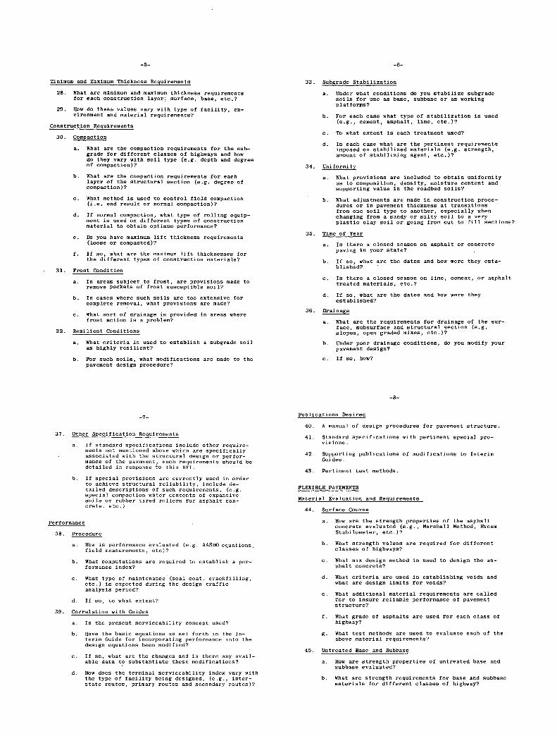
-5- -6-

Minimum and Maximum Thickness Requirements 33. Subgrade Stabilization

28. What are minimum and maximum thickness requirements a. Under what conditions do you stabilize subgrade for each construction layer; surface, base, etc.? soils for use as base, subbase or as working

platforms? 29. 110w do these valuew vary with type of faciiity, en-

vironment and material requirements? b. For each case what type of stabilization is used (e.g., cement, asphalt, lime, etc.)?

Construction Requirements C. To what extent is each treatment used?

30. Compaction d. In each case what are the pertinent requirements

a. What are the compaction requirements for the sub- imposed on stabilized materials (e.g. strength, grade for different classes of highways and how an,ount of stabilizing agent, etc.)? do they vary with soil type (e.g. depth and degree of compaction)? 34. Uniformity

b. What are the compaction requirements for each a. What provisions are included to obtain uniformity layer of the structural section (e.g. degree of as to composition, density, moisture content and compaction)? supporting value in the roadbed soils?

c. What method is used to control field compaction b. What adjustments are made in construction proce- (i.e. end result or normal compaction)? dures or in pavement thickness at transitions

from one soil type to another, especially when d. If normal compaction, what type of rolling equip- changing from a sandy or silty soil to a very

ment is used on different types of construction plastic clay soil or going from Cut to fill sections? material to obtain optimum performance?

35. Time of Year e. lb you have maximum lift thickness requirements

(loose or compacted)? a. Is there a closed season on asphalt or concrete

f. If so, what are the maximum lift thicknesses for paving in your state?

the different types of construction materials? b. If so, what are the dates and how were they esta-

blished? 31. Frost Condition

C. Is there a closed season on lime, cement, or asphalt In areas subject to frost, are provisions made to treated materials, etc.? remove pockets of frost susceptible soil?

In cases where such soils are too extensive for d. If, what are the dates and how were they tso

complete removal, what provisions are made? es ab li shed?

36. Drainage c. What sort of drainage is provided in areas where

frost action is a problem? a. What are the requirements for drainage of the sur- face, subsurface and structural section (e.g.

32. Resilient Conditions slopes, open graded mixes, etc.)?

a. What critoria is used to establish a subgrade soil b. Under poor drainage conditions, do you modify your as highly resilient? pavement design?

b. For such soils, what modifications are made to the c. If so, how? pavement design procedure?

-8-

-7- Publications Desired

40. A manual of design procedures for pavement structure.

37. Other Specification Requirements 41. Standard specifications with pertinent special pro-

a. If standard specifications include other require- Vi5iOfl5•

cents not mentioned above which are Specifically associated with the structural design or perfor- 42. Supporting publications of modifications to Interim macce of the pavement, such requirements should be Guides detailed in response to this sF1.

43. Pertinent test methods. b. If special provisions are currently used in order

to achieve structural reliability, include de- tailed descriptions of such requirements, (e.g. FLEXIBLE PAVEMENTS special compaction water contents of expansive soils or rubber tired rollers for asphalt con- Material Evaluation and Requirements

crete. etc.) 44. Surface Course

Performance a. How are the strength properties of the asphalt concrete evaluated (e.g. Marshall Method, Hymen

38. Procedure Stabilometer, etc.)?

a. How is performance evaluated (e.g. AASHO equations, b. What strength values are required for different field measurements, etc)? classes of highways?

b. What computations are required to establish a per- C. What mix design method is used to design the as- formance index? phalt concrete?

C. What type of maintenance (seal coat, crackfiilisg, d. What criteria are used in establishing voids and etc.) is expected during the design traffic what are design limits for voids? analysis period?

e. What additional material requirements are called d. If so, to what extent? for to insure reliable performance of pavement

structure? 39. Correlation with Guides

f. What grade of asphalts are used for each class of Is the present serviceability concept used? highway?

Have the basic equations as set forth in the In- g. what test methods are used to evaluate each of the terim Guide for incorporating performance into the above material requirements? design equations been modified?

45. Untreated Base and Subbase C. If so, what are the changes and is there any avail-

able data to substantiate these modifications? How are strength properties of untreated base and subbase evaluated?

d. How does the terminal serviceability index vary with the type of facility being designed, (e.g., inter- What are strength requirements for base and subbase state routes, primary routes and secondary routes)? materials for different classes of highway?

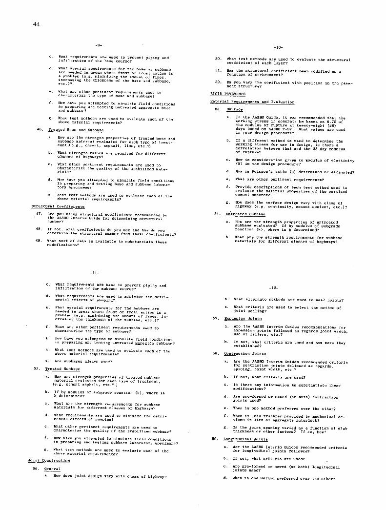
-10-

44

C. What requirements are used to prevent piping and infiltration of the base Course?

What special requirements for the base or subbase are needed in areas where frost or frost action is a problem (e.g. minimizing the amount of fines, increasing the thickness of the base and subbase, etc.)?

What are other pertinent requirements used to characterize the type of base and subbase?

How have you attempted to simulate field conditions on preparing and testing untreated aggregate base and subbase?

What test methods are used to evaluate each of the above material requirements?

46. Treated Base and Subbase

How are the strength properties of treated base and subbase material evaluated for each type of treat-ment,(e.g., cement, asphalt, line, etc.?)

What strength values are required for different classes of highways?

What other pertinent requirements are used to characterize the quality of the stabilized mate-rials?

How have you attempted to simulate field conditions on preparing and testing base and subbase labora-tory specimens?

What test methods are used to evaluate each of the above material requirements?

Structural Coefficients

47. Are you using structural coefficients recommended by the AASHO Interim Guide for determining structural number?

48. If not, what coefficients do you use and how do you determine the structural number from these coefficients?

49. What sort of data is available to substantiate these modificationo?

50. What test methods are used to evaluate the structural coefficient of each layer?

51. Has the structural coefficient been modified as a function of environment?

52. Do you vary the coefficient with position in the pave-ment structure?

RIGID PAVEMENTS

Material Requirements and Evaluation

53. Surface

In the AASHO Guide, it was recommended that the working stress in concrete be based on 0.75 of the modulus of rupture at twenty-eight (28) days based on AASHO T-97, What values are used in your design procedure?

If a different method is used to determine the working stress for use in design, is there a correlation between that and the 28 day modulus of rupture?

How is consideration given to modulus of elasticity (E) in the design procedure?

How is Poisson's ratio ('i) determined or estimated?

What are other pertinent requirements?

Provide descriptions of each test method used to evaluate the material properties of the portland cement concrete.

How does the surface design vary with class of highway (e.g. continuity, cement Content, etc.)?

54. Untreated Subbase

How are the strength properties of untreated subbase evaluated? If by modulus of subgrade reaction (k), where is k determined?

What are the strength requirements for subbase materials for different classes of highways?

C. What requirements are used to prevent piping and infiltration of the subbase course?

What requirements are used to ninimize the detri-sental effects of pumping?

What special requirements for the subbase are needed in areas where frost or frost action is a problem (e.g. minimizing the amount of fines, in-creasing the thickness of the subbase, etc.)?

What are other pertinent requirements used to characterize the type of Subbase?

How have you attempted to simulate field conditions on preparing and testing untreated aggregate subbase?

What test methods are used to evaluate each of the above material requirements?

Are subbases always used?

55. Treated Subbase

How are strength properties of treated subbase material evaluated for each type of treatment,

(e.g. cement asphalt, etc.?

If by modulus of subgrade reaction (k) where is k determined?

What are the strength requirements for subbase materials for different classes of highways?

What requirements are used to minimize the detri-mental effects of pumping?

What other pertinent requirements are used to characterize the quality of the Stabilized subbase?

How have you attempted to simulate field conditions in preparing and testing subbase laboratory specinens?

What test methods are used to evaluate each of the above material requirements?

Joint Construction

56. General

a. How does joint design vary with class of highway?

-12-

b. What alternate methods are used to seal joints?

C. What criteria are used to select the method of joint sealing?

57. Expansion Joints

Are the AASHO Interim Guides recommendations for expansion joints followed as regards joint width, use of fillers, etc.?

If not, what criteria are used and how were they established?

58. Contraction Joints

Are the AASHO Interim Guides recommended criteria for contraction joints followed as regards. spacing, joint width, etc.?

If not, what criteria are used?

C. Is there any information to substantiate these modifications?

Are pre-formed or sawed (or both) contraction joints used?

When is one method preferred over the other?

When is load transfer provided by mechanical de-vices in lieu of aggregate interlock?

Is the joint spacing varied as a function of slab thickness or other factors? If so, how?

59. Longitudinal Joints

Are the AASHO Interim Guides recommended criteria for longitudinal joints followed?

If not, what criteria are used?

C. Are pre-formed or sawed (or both) longitudinal joints used?

d. When is one method preferred over the other?

-13-

60. Load Transfer Devices

Are the AASHO Interim Guides recommended criteria for mechanical load transfer devices followed as regards diameter, length and spacing?

If not, what criteria are used?

C. Are typical drawings of joints with mechanical load transfer devices available?

a. What means is provided to prevent corrosion where salt is applied to the surface of the pavement?

61. Tiebars

Are the AASHO Interim Guides recommendations for tiebars followed as regards bar sizes, length and spacing?

U. not, what modifications have been made?

C. Are the Interim Guide's recommendations regarding strength of steel used?

If not, what modifications have been made?

What means is provided to prevent corrosion where salt is applied to the surface of the pavement?

Reinforcement

62. ReinfOrced Concrete Pavement

Do you follow the AASHO Interim Guide's design charts for percent steel or slab?

If not, what criteria do you use?

63. Continuously Reinforced Concrete Pavement

Are the AASHO Interim Guide's design charts folloo as regards percent steel in continuously reinforced concrete pavement?

If not, what criteria do you use?

45

-14-

Continuity Effect on Slab Thickness

a. Is there any incremental adjustments provided for in slab thickness requirements as a function of slab continuity, (e.g., jointed pavements, rein-forced concrete pavements, continuously reinforced Concrete pavement?)

Terminal Treatment

Is any special terminal treatment of the concrete pave-ment used at bridges or other fixed objects, e.g., terminal anchorage, piles, etc.?

If so, what criteria-are used?

OVERLAYS (Of Existing Flexible or Rigid Pavements)

Design Procedures

What procedure is used to evaluate the existing pave-ment for purposes of estimating overlay requirements

(e.g., experience, deflection, strain in surface course or subgrade? )

What tests or experience factors are used to evaluate properties of existing pavements?

What are the required surface preparation requirements prior to overlay, (e.g., subsealing, patching or "breaking" the pavement?

What are minimum requirements for overlays (either flexi-ble or rigid)?

FUTURE RESEARCH

Are there any projects (current or proposed) from which data will be used to revise the current design procedure?

If so, what are they?

a a

.00 Cu 4.40 06. a 00

01 1< 04-I 10.-I

(1

'o 0

0 #40 4<

0< 1< 0<0<1< <1<H 4<4

04 H

<04040<1< (0 14041< 14 1< 1<1<1<

0<0< 0< 0<1< H 1< 1< 1< (<H

.0 a 00

00 0 0 (0 0 0 0 00 0 #1 4, -In 000.-I 00

1

0 'I-I 0 o n 00 0 0. .05. 0 00 0000 0 0-' 00 0 - 0 00 (0 0.00 000) 0 41.0 00-441 .50 0(00 .4 0 (00 0,01 (0 ('0 V 000.41.4 .4 00 0.10 .4.S0000 >1000 000 00441 -4 .1.4(0

00004 041410000 •400 .000 0 .000(0041 aS 64.. 5400 (0 -44000 DIR (0000(00 00000V., 41 00 100,4 00 0(0(00000 01000000 00 00>. 00 0 00>00 .O (0 n.SO0'I., Ioa8..Ib.0 ,00000 0000000,.I 00.44100 00000Z 444 (0>0.0 .00000.0 .00(0 0 '-4-4 0-I 411.1 .4 .010500.4 00004141 00.0,44100 1041.10>. 10.0000(0 #4 4,00 1.41.40 00b00V44 4.Inm.on (0.04100 #141 00

0000.4.5.-I .10-100 800,-low 0000.441 00010010 0.0>55 554141.. ,-I00000 000(00041 41(011000 00 #4

,.4.-414-400 000-4(1 00v,-400 00000000 n -I .5 '4-4 000001 0000.0 .5410110 000410 .4000,-Ia. .43 0 00D1. (010>410- 14(04.1(0(0 (0(0(0(0(0 (0Z(0ZZ ZZS;(00 000.1010 a4EE-1> (-(010mw 06.

Use B.P.R. Modification Guides

x

x

x

x

--

Do not Use Guides

x

x x

x

(3) (3)

x

TABLE A-2

USE OF INTERIM GUIDES' WHEEL LOAD EQUIVALENCE FACTORS

Agency Use Guides

Alabama X Alaska Arizona X Arkansas X California

Colorado Connecticut Delaware X Florida Georgia X

Hawaii Ida ho Illinois X Indiana X Iowa X

Kansas Kentucky X Louisiana X Maine X Maryland S

Massachusetts X Michigan (I Mississippi X Minnesota Missouri X

Montana X Nebraska X Nevada X New Hampshire X New Jersey X

New Mexico X New York North Carolina X North Dakota Ohio X

Oklahoma Oregon Pennsylvania X Rhode Island South Carolina

South Dakota X 1 Tennessee X 1 Texas X Utah X Vermont

Virginia Washington West Virginia Wisconsin X Wyoming X

Districtof Columbia Puerto Rico X

TOTALS:

U) Used in checking design only 2 Use for special studies Use Calif. Equivalency Factors

TABLE A-3

WHEEL LOAD USED FOR PAVEMENT DESIGN

Flexible Pavements Rigid Pavements

k Heaviest Axle Loads I Agency Axle Load Wheel Load Other None 18 PCA Type Concept None

Alabama X X Alaska X

X Arizona X X Arkansas X X California X X

Colorado X X Connecticut x X Delaware X X Florida x X Georgia X x

Hawaii X X Idaho X X Illinois X x Indiana X X Iowa X X

Kansas X X

Kentucky X X Louisiana X X Maine X X Maryland S X

Massachusetts X X(l) Michigan (3) X X Mississippi X X Minnesota

(3) X X - Missouri X X

Montana X X Nebraska X x Nevada X X New Hampshire X X(2) New Jersey X X

New Mexico X (2) X

New York X X North Carolina X x North Dakota X X Ohio X X

Oklahoma X X Oregon X X Pennsylvania X X Rhode Island X X South Carolina X X

South Dakota X (3) X (3 Tennessee X X 3 Texas X X Utah X X (1) Vermont X X

Virginia X X Washington X X (2)

West Virginia X X Wisconsin X X Wyoming X X

District of Columbia Puerto Rico X X

TOTALS -s-. T7

TABLE A-5

OTHER METHODS FOR ESTABLISHING SOIL SUPPORT

Other Pedo- Soil logical Classi- Classi- Frost Standard

Agency fications fications Index Section Experience

Alaska X Connecticut x Iowa x Michigan X Minnesota X

New York X North Dakota X Oklahoma X Rhode Island X Vermont X

District of Columbia X

TOTALS 4 1 1 1 4

TABLE A-4

TEST METHODS USED TO ESTABLISH SOIL SUPPORT

Agency CBR R-Value Triaxial Group Index Other

Alabama X Alaska X Arizona X Arkansas X California X

Colorado X X Connecticut Delaware X Florida X Georgia X X

Hawaii X Idaho X Illinois X Indiana X Iowa X

Kansas X Kentucky X Lou isiana X Maine X Maryland X

Massachusetts X Michigan X Mississippi X Minnesota X Missouri X

Montana X Nebraska X Nevada X New Hampshire X New Jersey X

New Mexico X New York X North Carolina X X North Dakota X

Ohio X

Oklahoma X Oregon X Pennsylvania x Rhode Island X South Carolina x

South Dakota X Tennessee X Texas X Utah X Vermont X

Virginia X Washington X West Virginia X Wisconsin X Wyoming X

District of Columbia X Puerto Rico X - --

TABLE A-6 TABLE A-7

PROCEDURES USED TO INCORPORATE SOIL SUPPORT AVAILABLE CORRELATION BETWEEN TEST METHODS INTO DESIGN METHOD

CBR vs Soil CBR vs R-Value vs

Agency Use Interim Guides Use California Method Other Aency Classification K-Value K-Value -

Alabama x Alabama X Alaska x Alaska

Arizona X 2 X

Arizona Arkansas

x X Arkansas X(l)

California x California X

Colorado Colorado x Connecticut Connecticul x Delaware x Delaware x Florida x Florida (3) X Georgia x Georgia x

Hawaii x Hawaii X X Idaho x Idaho X X Illinois x Illinois x Indiana x Indiana X Iowa X Iowa x

Kansas x Kansas

Kentucky Kentucky Louisiana x Louisiana

Maine x Maine - x Maryland x Maryland x

Massa chuse t ts X Massachusetts

Michigan x Michigan x Minnesota x Minnesota x Mississippi x MississippE X Missouri Missouri x

Montana x Montana x Nebraska x Nebraska x Nevada x Nevada x New Hampshire x New HampshIre

New Jersey x New Jersey X

New Mexico X New Mexico x New York x New York x North Carolina X North Carolina x North Dakota x North Dakota X Ohio X Ohio X

Oklahoma x Oklahoma X Oregon x Oregon x Pennsylvania x PennsylvanIa x Rhode Island x Rhode Islaid x South Carolina South Carolina x

South Dakota x South Dakota x Tennessee x Tennessee

Texas x Texas X(1) Utah x Utah x Vermont x Vermont x

Virginia x Virginia x Washington x Washington. x West Virginia x West Virginia x Wisconsin X Wisconsin x Wyoming x Wyoming x

District of Columbia x District of Columbia x Puerto Rico X Puerto Roci X

-- -- 28 TOTALS 31 6 13

0 Studias underway 3 Triaxial Test vs Support Value * For checking purposes only 2 R-Va1ue vs P1 and Gradation 4 CBR vs Support Value

(5) Group Index vs Support Value

TABLE A-9

AGENCIES THAT HAVE ESTABLISHED INTRASTATE REGIONAL FACTORS

Arizona Ii. New Hampshire Georgia 12. New Mexico Hawaii 13. North Carolina Idaho 14. Oklahoma

TABLE A-8 Iowa 15. South Dakota

USE OF INTERIM GUIDES' RECOMMENDATIONS TO ESTABLISH : nd : Wyoming

A REGIONAL FACTOR S. Massachusetts 18. Puerto Rico Michigan Nebraska

From Guides, From Other Regional Factors Agency From Guides Modified Sources Not Used

Alabama X TABLE A-b Arizona X

IN DETERMINING REGIONAL FACTOR Arkansas x FACTORS CONSIDERED California X

Colorado X Connecticut X C 5 0

Delaware X ' Florida X Georgia X bO .404) 04 44) 0) 04. 4,

0 06

0 - 10

x 0 •ebOa C CO 0. 5 4) '.4 00

0. on 5 04)

on 000

Hawaii Idaho X Agency E.

Illinois X X Indiana X Alabama

Iowa x Alaska X Arizona X X

Kansas x Arkansas N

Kentucky X Delaware N

Lou isiana X x Georgia X X X X Maine

Maryland x Hawaii X Idaho X X

Massachusetts X Illinois X

Michigan x Indiana X

Minnesota X - X

Mississippi X Iowa X Missouri It Kansas X X

Montana X Kentucky Louisiana X

X Nebraska X Maine X

Nevada New Hampshire

X X Maryland It

New Jersey X Massachusetts X Michigan X X

New Mexico X Mississippi X

New York x Montana X X x North Carolina X x x North Dakota X Nebraska

X Ohio X Nevada X X

New Hampshire X It

Oklahoma X New Jersey It

Oregon X New Mexico X X X

Pennsylvania x X Rhode Island X North Carolina X

South Carolina x North Dakota It

Ohio X

South Dakota x Oklahoma X

Tennessee X Pennsylvania It

Texas Utah

X x South Carolina It

Vermont X South Dakota X X Tennessee X

Virginia X Texas X

It

X Washington X Utah West Virginia X

It Wisconsin X Virginia X

Wyoming X Wisconsin Wyoming X X X

District of Columbia x Puerto Rico X

Puerto Rico X - - TOTALS: 14 18 6 14 TOTALS 5 5 13 5 5 2 4 13 3 5

TABLE A-li

TABLE A-12

METHODS USED IN DESIGN PROCEDURE TO CONSIDER EFFECT

REQUIRED THICKNESS OF OF FROST PENETRATION

NON-FROST-SUSCEPTIBLE MATERIAL

Use Granular Agency Regional Factor Material Not Considered

Alabama Alaska x Arizona X Arkansas California x

Colorado x Connecticut x Delaware x Florida Georgia

Hawaii Idaho X Illinois x Indiana x Iowa X

Kansas x Kentucky x Lou isiana Maine x Maryland x

Massachusetts X Michigan x Minnesota X Mississippi Missouri x

Montana X Nebraska X Nevada x New Hampshire x New Jersey X

New Mexico X New York x North Carolina North Dakota X Ohio x

Oklahoma x Oregon x Pennsylvania x Rhode Island x South Carolina

South Dakota X Tennessee x Texas Utah x Vermont x

Virginia X Washington x West Virginia x Wisconsin X Wyoming X

Districtof Columbia X Puerto Rico

TOTALS: 7

Corps of Not a Problem % of Frost Depth Standard Engineers

x Agency 50 67 75 100 277 3 Procedure Experience

Alaska X

X California X Colorado X Connecticut K Iowa X

Maine X

x Maryland X X Michigan X Minnesota X Montana X

Nevada x(l\ (2) New Hampshire X x New Jersey X New York X X Oregon X

x Pennsylvania X Rhode Island X Utah X Washington X West Virginia x

Wisconsin X

x

'Secondary Roads

(2) Interstate

x

x

x

TABLE A-14

STRUCTURAL LAYER COEFFICIENT CONCEPTS USED BY AGENCIES NOT USING THOSE RECOMMENDED BY THE GUIDES

TABLE A-13

USE OF INTERIM GUIDES' STRUCTURAL LAYER COEFFICIENTS

Use Guides With Use Guides, But Agency Use Guides Modification Not For Design Do Not Use

Alabama X Alaska X Arizona X Arkansas X California X

Colorado X Connecticut x Delaware X Florida X Georgia X

Hawaii X Idaho X Illinois X Indiana X Iowa x - Kansas Kentucky X

X Lou isiana Maine X Maryland X

Massachusetts X Michigan X Minnesota (2' x Mississippi X(1) Missouri X

Montana X Nebraska X Nevada X New Hampshire X New Jersey X

New Mexico X New York X North Carolina x North Dakota X Ohio X

Oklahoma x Oregon x Pennsylvania X Rhode Island X South Carolina x

South Dakota x 2 Tennessee x 2 Texas x Utah X Vermont X

Virginia x Washington X West Virginia X Wisconsin X Wyoming X

Districtof Columbia x Puerto Rico x

TOTALS T

Use for special studies 2 Use for checking design

California Gravel Other Gravel Do not use Equivalency Concept Equivalency Concepts Equivalency Concept

California Minnesota Alaska

Hawaii Oklahoma Colorado

Idaho Virginia Connecticu;

Oregon District of Columbia

Washington Florida

West Virginia Michigan

New York

Rhode Island

Vermont

TABLE A-16

SUMMARY OF STATES USING STRENGTH TEST TO ESTIMATE STRUCTURAL LAYER COEFFICIENT

S 5 0 - 0 n.e -

S 0 wH

a SC a C 2 a -

m 1.5 as

5 a mm

1. H 51. o 1.0

a 0

Agency _ .-.

Alabama X

Arizona X

Illinois X X X

Louisiana X x New Mexico X X

Ohio IC

Texas X X

Wyoming X X LA

TABLE A-15

SUMMARY OF STRUCTURAL LAYER COEFFICIENTS USED FOR DIFFERENT PAVEMENT COMPONENTS

SURFACE COURSES

PLANT MIX ROAD MIX (HIGH (LOW

STATE STABILITY) - STABILITY) OTHER

0.44 0.20 Sand asphalt 0.40

0.35-0.44 0.25-0.38 Sand asphalt 0.25

0.35-0.40

0.44 -

0.315 -

0.30-0.35 0.20

Plant-mix sand asphalt (low stab.) 0.28

Nevada 0.30-0.35 0.17-0.25 -

New Hampshire 0.38 0.20 Sand asphalt 0.20

New Mexico 0.30-0.45 0.20 Plant-mix seal 0.25

Ohio 0.40 -

Pennsylvania 0.44 0.20 Sand asphalt 0.35

South Carolina 0.40 - A. C. binder 0.35 sand asphalt

South Dakota 0.36-0.42 - -

BASE COURSES

UNTREATED

Limestone - 0.14 Slag 0.14 Sandstone 0.13 Granite 0.12

Sand & gravel, well graded 0,14

Cinders 0.12-0,14 Sandy gravel, mostly

sand 0.11-0.13 Waterbound macadam 0.20 Crusher run 0.14 Quarry waste 0.11 Select borrow 0.08 Crushed stone 0.14

Crushed rock (Class 5 &6gravel) 0.14

Sandy gravel 0.07

Crushed gravel <1½" 0.14 > 1½" 0.12

Select surf. 0.10 Spec. borrow 0.07 Sand 0.05 Crushed gravel 0.10-0.12 Crushed rock 0.13-0.16 Crushed gravel 0.10 Bank run gravel 0.07 Crushed stone 0.14 Quarry rock 0.10-0.15 Crushed rock 0.06-0.12

Aggregate 0.14 Waterbound macadam 0.14 Crushed stone 0.14 Dense grade 0.18

Crushed rock 0.14

0.11

Alabama

Arizona

Delaware

Massachusetts

Minnesota

Montana

Utah 0.40 0.20 Plant-mix seal 0.40 0.12

Wisconsin 0.44 0.20 Sand asphalt 0.40 Crushed gravel 0.10 Crushed stone 0.14 Waterbound macadam 0.15-0.20 Sand-gravel uncrushed 0.07

Wyoming 0.30-0.40 - Inverted penetration 0.20-0.25 0.05-0.12

Notes: Consult AASHO Interim Guide (86, Table A 4-1) for values Used by the following states: I. Indiana, Iowa, New Jersey, Tennessee, and Puerto Rico-values as shown.

North Carolina and North Dakota-values as shown, except 0.30 for bituminous-treated base. Maine-values as shown, with some modifications. Maryland-substitution values for materials to replace design thickness of asphalt hot.mix are the AASHO structural coefficients expressed in layer

thicknesses, in inches.

CEMENT-TREATED LIME-TREATED BITUMINOUS-TREATED SUBBASES

<400 psi 0.15 - Coarse graded 0.030 Sand & sandy clay 0.11 400-650 psi 0.20 Sand 0.25 Chert, low P.1. 0.10 > 650 psi 0.23 Topsoil 0.09

Float gravel 0.09 Sand & silty clay 0.05

< 300 psi 0.15 - Sand-gravel 0.25-0.34 Sand-gravel, well 300-500 psi 0.18-0,25 Sand 0.20 graded 0.14 > 500 psi 0.25-0.30 Crushed stone or

cinders 0.12 Sand & silty clay 0.05-0.10

Soil-cement 0.20 - Asph. stab. 0.10 Select borrow 0.08

- - Blackbase 0.34 Gravel 0.11 Penetrated crushed stone 0.29 Select material 0.08

- - 0.175-0.21 Sandy gravel (C1.3 & 4 gravel) 0.105

Selected granular (<12% minus #200) 0.07

<400 psi 0.15 0.15 Plant mix 0.25-0.30 - > 400 psi 0.20 Bit. stab. 0.20

- - Plant mix 0.25-0.34 Gravel type 1 0.09-0.11 Select material 0.05-0.09

Gravel 0.17 - Bit. conc. 0.34 Sand-gravel 0.05 Gravel 0.24

<400 psi 0.12 0.05-0.10 Plant mix 0.30 Aggregate 0.06-0.12 400-650 psi 0.17 Road mix 0.15 Borrow 0.05-0.10 > 650 psi 0.23

- - - 0.11

Soil-cement 0.20 Soil-lime Soil-bit. 0.20 Sand-gravel 0.11 Cement aggr. 0.20 Plant mix 0.30

plant mix 0.30 - - Black base 0.30 -

Sand 0.25

0.20 0.18 Hot mix Untreated 0.10 aggregate 0.30 coarse sand 0.24 fine sand 0.18

Cold mix aggregate 0.15

400-650 psi 0.20 - Coarse graded 0.30 Sand-gravel 0.10 Sand or sandy clay 0.06-0.10

<400 psi 0.15 0.15-0.30 Coarse graded plant mix 0.34 Sand-gravel 0.05-0.11 400-650 psi 0.20 Sand plant mix 0.30 > 650 psi 0.23

0.15-0.25 0.07-0.12 Plant mix 0.20-0.30 Special borrow 0.05-0.12 Emulsion 0.12-0.20

TABLE A-18

CRITERIA FOR VARYING STRUCTURAL LAYER COEFFICIENTS WITH POSITION IN PAVEMENT STRUCTURE

Agency Criteria

Alabama No indication

Arizona For sandwich-type construction - CTB

Georgia No indication

Illinois Gravel material has a different coefficient when used as base than when used as surface material (inherent when specifying) minimum thickness re- quirements

Kansas No indication - Guides used on special studies only

Louisiana No indication

Maryland Inherent when specifying minimum thickness re- quirements

Nevada No indication

South Carolina On overlays

South Dakota Subbase gravel used adjacent to subgrade has a coefficient of 0.11 with base. Coarse gravel (with a better gradation) is given a value of 0.10

Washington Empirical Equation

Wyoming Considered in selecting structural coefficients within the overall allowable range

Puerto Rico No indication

TABLE A-17

VARIATION IN STRUCTURAL LAYER COEFFICIENT WITH POSITION IN PAVEMENT STRUCTURE

Vary Structural Do Not Vary Agency Coefficient Structural Coefficient Concept Not Used

Alabama X Alaska X Arizona X Arkansas X California X

Colorado X connecticut X Delaware X Florida X Georgia X

Hawaii X Idaho X Illinois X Indiana X Iowa X

Kansas X Kentucky X Louisiana X Maine X Maryland X

Massachusetts X Michigan X Minnesota X Mississippi X Missouri X

Montana X Nebraska X Nevada X New Hampshire x New Jersey X

New Mexico X New York S North Carolina X North Dakota X Ohio X

Oklahoma X Oregon X Pennsylvania X Rhode Island N South Carolina X

South Dakota x Tennessee X Texas X Utah X Vermont S

Virginia X Washington X West Virginia X Wisconsin X Wyoming X

District of Columbia S Puerto Rico X

TOTALS

TABLE A-19

PROCEDURE USED TO DETERMINE WORKING STRESS IN PORTLAND CEMENT CONCRETE

Guides California Assume Constant PCA Standard Agency Method Method Working Stress Method Section None Other

Alabama X Alaska X Arizona X Arkansas X California X

Colorado X Connecticut N Delaware X Florida X Georgia X

Hawaii X Idaho X Illinois X Indiana X (2) Iowa X

Kansas X Kentucky X Louisiana X Maine N Maryland X

Massa c huset ts Michigan X Minnesota N Mississippi X Missouri X

X 2 Montana Nebraska X Nevada X New Hampshire x New Jersey X

New Mexico X New York X North Carolina X North Dakota X Ohio X

Oklahoma X 2 x oregon Pennsylvania X Rhode Island X South Carolina X

South Dakota X Tennessee X Texas Utah X Vermont

Virginia N Washington N West Virginia X 3 Wisconsin X Wyoming X

Districtof Columbia x Puerto Rico X

TOTALS - -r 55(1) T

1 Rigid Pavements not used 3 Combination of PCA, AASHO, and experience

2 Compressive Strength 4 For checking design or.ly

TABLE A-20

METHODS OF DETERMINING k-VALUE FOR RIGID PAVEMENT DESIGN

CBS S-Value Triaxial Soil Rigid Measure Assume Corre- Corre- Corre- Classification Pavement K-Value

Agency Insitu Experience lation lation lation Correlation Not Used Not Used

Alabama X Alaska X Arizona X(l) Arkansas X (1) California X

Colorado X Connecticut X Delaware Florida

N X

Georgia

Hawaii X 1 Idaho X Illinois (2) X Indiana X Iowa X

Kansas X Kentucky X Lou isiana X Maine X Maryland X

Massachusetts x Michigan X Minnesota X Mississippi X Missouri X

Montana X Nebraska X Nevada X New Hampshire X New Jersey X

New Mexico New York X North Carolina X 3 North Dakota X Ohio N

Oklahoma X Oregon X Pennsylvania X Rhode Island (1) X South Carolina x

South Dakota X Tennessee X Texas X Utah X Vermont X

Virginia N Washington X West Virginia X Wisconsin X Wyoming X

District of Columbia N Puerto Rico X

TOTALS 1 9 15 7 2

'Use only stabilized subbases

not credit the granular subbase

3>Subbase not used extensively UI UI

TABLE A-21

EXTENT OF USE OF GUiDES' RECOMMENDATIONS FOR STEEL IN REINFORCED CONCRETE PAVEMENTS

Use Guides Do Not Use Agency Recommendations Guides Recommendations

Alabama Alaska Arizona Arkansas California

Colorado Connecticut Delaware Florida Georgia

Hawaii Idaho Illinois Indiana Iowa

Kansas Kentucky Louisiana Maine Maryland

Massachusetts Michigan Minnesota Mississippi Missouri

Monta ma Nebraska Nevada New Hampshire New Jersey

New Mexico New York North Carolina North Dakota Ohio

Okla homa Oregon Pennsylvania Rhode Island South Carolina

South Dakota Tennessee Texas Utah Vermont

Virginia Washington West Virginia Wisconsin Wyoming

District of Columbia Puerto Rico

TOTALS

RCP Not Used

x x x x

x x

x x

x

x

x x

x

x

x

x

x

x

14

TABLE A-22

EXTENT OF USE OF GUIDES' RECOMMENDATIONS REGARDING CONTINUOUS REINFORCED CONCRETE PAVEMENTS

Use Guides Do Not Use Guides Agency Recommendations Recommendations Do Not Use CRCP

Alabama X Alaska X Arizona X Arkansas X California X

Colorado X Connecticut x Delaware X Florida X Georgia X

Hawaii X Idaho X Illinnis X Indiana X Iowa X

Kansas X Kentucky X Louisiana X Maine X Maryland X

Massachusetts x Michigan X Minnesota X Mississippi X Missoiri X

Montana X Nebraska X Nevada X New Hampshire x New Jersey X

New Mexico X NewYork X North Carolina X North Dakota X Ohio X

Oklahoma X Oregon X Pennsylvania X Rhode Island X South Carolina X

South Dakota X Tennessee X Texas X Utah X Vermont X

Virginia X Washington X West Virginia X Wiscomsin X Wyoming X

District of Columbia X Puerto Rico - X

TOTALS 10

TABLE A-24

SUBDIVISION OF EXPERIENCE METHOD FOR OVERLAY DESIGN

Ridability Condition Survey

Idaho Idaho

Massachusetts Kansas

Michigan Maryland

Minnesota Massachusetts

Montana Michigan

North Dakota Minnesota

Ohio Montana

Rhode Island Nebraska

West Virginia Nevada

Ohio

West Virginia

TABLE A-23

METHOD(S) OF OVERLAY DESIGN USED

AASHO AASHO Agency Deflection Flexible Psi Experience Visual

Alabama X X Alaska X Arizona x Arkansas X California X X

Colorado X Delaware X Florida

* X x

Georgia X Hawaii X X

Idaho X x Illinois X Indiana x Iowa x Kansas x

Kentucky * X Louisiana X X Maine * X Maryland X X Massachusetts X

Michigan * X Minnesota X X Mississippi X Missouri X Montana X

Nebraska X Nevada X New Hampshire x New Jersey * X X New Mexico X X

NewYork X North Carolina x North Dakota X - Ohio x Oklahoma X X

Oregon x Pennsylvania x Rhode Island X South Carolina x South Dakota X

Texas X x Utah X Vermont x Virginia * X Washington X X

West Virginia xt x Wisconsin X Wyoming X District of Columbia X Puerto Rico X

TOTALS: 11

*Secondary Method

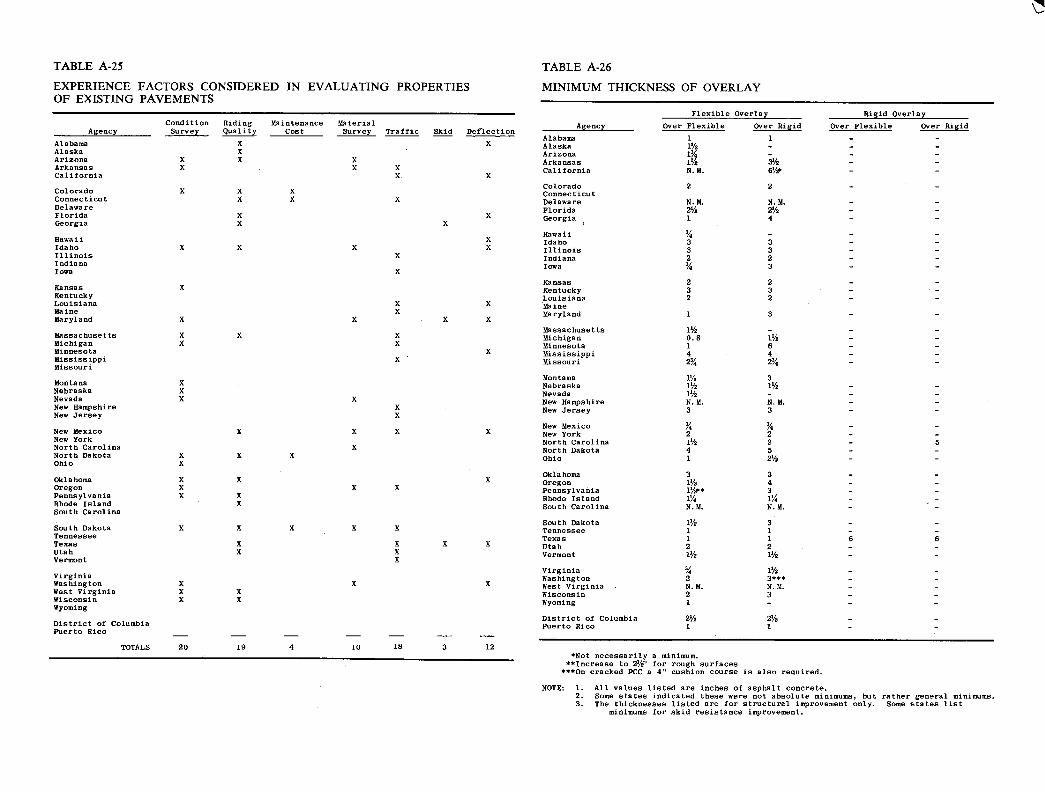
TABLE A-25

EXPERIENCE FACTORS CONSIDERED IN EVALUATING PROPERTIES OF EXISTING PAVEMENTS

Condition Riding Maintenance Material Agency Survey Quality Cost Survey Traffic Skid Deflection

Alabama X X Alaska X Arizona X X X Arkansas X X X California X X

Colorado X X X Connecticut X X X Delaware Florida X X Georgia X X

Hawaii X Idaho X X X x Illinois X Indiana Iowa X

Kansas X Kentucky Louisiana X X Maine X Maryland X X X X

Massachusetts X X X Michigan X X Minnesota X Mississippi X Missouri

Montana X Nebraska X Nevada X x New Hampshire X New Jersey X

New Mexico X X X X New York North Carolina X North Dakota X X X Ohio X

Oklahoma X X X Oregon X X X Pennsylvania X X Rhode Island X South Carolina

South Dakota X X X X X Tennessee Texas X X X X Utah X X Vermont X

Virginia Washington X X X West Virginia X X Wisconsin X X Wyoming

District of Columbia Puerto Rico

TOTALS 20 19 4 10 18 3 12

TABLE A-26

MINIMUM THICKNESS OF OVERLAY

Flexible Overlay Rigid Overlay

Agency Over Flexible Over Rigid Over Flexible Over Rigid

Alabama 1 1 - - Alaska 1% - - - Arizona j3/ - - - Arkansas 3½ - - California N.M. 6'/a* - - Colorado 2 2 - - Connecticut Delaware N.M. N.M. - - Florida 2'/z - - Georgia 1 4 - - Hawaii % - - - Idaho 3 3 - - Illinois 3 3 - - Indiana 2 2 - - Iowa 3/4 3 - - Kansas 2 2 - - Kentucky 3 3 - - Louisiana 2 2 - - Maine Maryland 1 3 - - Massachusetts 1½ - - - Michigan 0.8 1½ - - Minnesota 1 6 - - Mississippi 4 4 - - Missouri 2% 23/4 - - Montana 3 Nebraska 1½ 1'/2 - - Nevada 1½ - - - New Hampshire N.M. N.M. - - New Jersey 3 3 - - New Mexico % % - - New York 2 2 - - North Carolina 1½ 2 - 5 North Dakota 4 5 - - Ohio 1 21/2 - - Oklahoma 3 3 - - Oregon 1½ 4 - - Pennsylvania 1'/* 3 - - Rhode Island 1'/4 l/4 - - South Carolina N.M. N.M. - - South Dakota 1½ 3 - - Tennessee 1 1 - - Texas 1 1 6 6 Utah 2 2 - - Vermont 11/2 1½ - - Virginia % 1½ - - Washington 2 3*5* - West Virginia N.M. N.M. - - Wisconsin 2 3 - - Wyoming 1 - - - District of Columbia 21/2 21/2 - - Puerto Rico 1 1 - -

SNot necessarily a minimum. **Increase to 21/i' for rough surfaces ***On cracked PCC a 4" cushion course is also required.

NOTE: 1. All values listed are inches of asphalt concrete. Some states indicated these were not absolute minimums, but rather general minimums. The thicknesses listed are for structural improvement only. Some states list

minimums for skid resistance improvement.

TABLE A-27

SUMMARY OF STATUS OF RESEARCH

Agency Current Research Proposed Research No Research

Alabama X Alaska X Arizona X Arkansas X California X

Colorado X Connecticut X Delaware X Florida X Georgia X

Hawaii X Idaho X Illinois X Indiana X Iowa X

Kansas X Kentucky X Maine X Maryland X

Massachusetts X Michigan X Minnesota X Mississippi X MIssouri X

Montana X Nebraska X Nevada X New Hampshire X New Jersey X

NewMexico X New York X North Carolina X North Dakota X Ohio X

Oklahoma X Oregon X Pennsylvania X Rhode Island x South Carolina X

South Dakota X Tennessee X Texas X Utah X Vermont x

Virginia X Washington x West Virginia X Wisconsin X Wyoming X

District of Columbia x Puerto Rico x

MWW<O 0.00 OZMMM MMMMM MMRt Cv.V.'OO N'' aOav.,- '<000,t 0wwa

00005 H000

00000 000)-.'- 05

00'lll)- EOnaqr

O - act -tow 1000010

0ctcc 50'OR

'1-twO) 0-,O'5Ot

0a.Ccct 0 0')-c

wa ,-,- ', S 5 0

5055w '1 5005

k '-0 00<0 '50 00

o'a 0)00010 waqSct 10 000'

av w0a, . QmW

-''101 5555 5551-'. 105 10 0aaS 1000'- 10 0010 ru 000 Or'1O' 5cc 0 0 '0 5 a ,< t•' - 000 ct

a,- 00 0 -

a a a a

I I Road Teat ru

N N N N N N N Correlation

icol N N I Satellite

Studies

IN x1 Frost Effects ru

z NiAggregates

Is N N ISIs Stabilization

I,)

I Quality Control

aol An I alysis of Mixed Traffic

a'! N Traffic

Projections

I Performance

N I< N ICRCP

0' Is 0< N I Joint Scalers

0'! > >4 N IJoint Design

< 0< 0< N Mix Design

N N N N Base Properties

N N ISubgrade Moisture

N N N N N Other

N N N ISoil Support

Structural NIs N N N N N Coefficients

N N Regional Factors

0 os N N N N Overlay Design

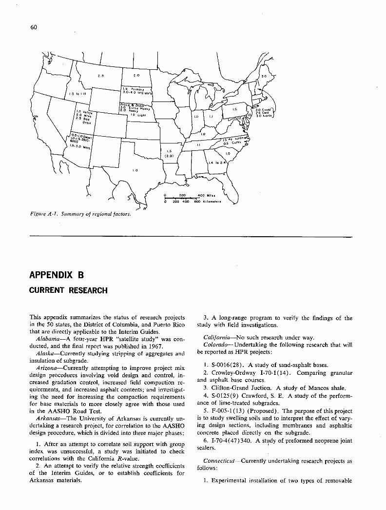
60

Figure A-I. Summary of regional factors.

APPENDIX B

CURRENT RESEARCH

This appendix summarizes the status of research projects in the 50 states, the District of Columbia, and Puerto Rico that are directly applicable to the Interim Guides.

Alabama—A four-year HPR "satellite study" was con-ducted, and the final report was published in 1967.

Alaska—Currently studying stripping of aggregates and insulation of subgrade.

Arizona—Currently attempting to improve project mix design procedures involving void design and control, in-creased gradation control, increased field compaction re-quirements, and increased asphalt contents; and investigat-ing the need for increasing the compaction requirements for base materials to more closely agree with those used in the AASHO Road Test.

Arkansas—The University of Arkansas is currently un-dertaking a research project, for correlation to the AASHO design procedure, which is divided into three major phases:

After an attempt to correlate soil support with group index was unsuccessful, a study was initiated to check correlations with the California R-value.

An attempt to verify the relative strength coefficients of the Interim Guides, or to establish coefficients for Arkansas materials.

A long-range program to verify the findings of the study with field investigations.

California—No such research under way. Colorado—Undertaking the following research that will

be reported as HPR projects:

S-0016(28). A study of sand-asphalt bases. Crowley-Ordway 1-70-1(14). Comparing granular

and asphalt base courses. Clifton-Grand Juction. A study of Mancos shale. S-0125(9) Crawford, S. E. A study of the perform-

ance of lime-treated subgrades. F-005-1(13) (Proposed). The purpose of this project

is to study swelling soils and to interpret the effect of vary-ing design sections, including membranes and asphaltic concrete placed directly on the subgrade.

1-70-4(47) 340. A study of preformed neoprene joint sealers.

Connecticut—Currently undertaking research projects as follows:

1. Experimental installation of two types of removable

61

joint formers, and sealing with extruded and closed-cell neoprene compression seals.

Study of density and depth control of bituminous concrete shoulders on penetration macadam and gravel bases.

Research conducted at the University of Connecticut to identify the causes of early deterioration of flexible pavement.

Continuing study of the performance of contraction design portland cement concrete pavement.

Study of rigid pavement finishing, particularly in regard to prevention of hydroplaning.

Delaware-Currently undertaking the following:

Determination of regional factor according to AASHO procedure.

Determination of the strength of select borrow and select borrow-cement stabilized base and subbase courses by evaluation of average CBR.

Land-use studies for Kent and Sussex Counties to improve projected traffic estimates.

Florida-Currently undertaking a flexible design re-search program.

Georgia-No such research under way. Hawaii-No such research under way. Idaho-No formal projects, but are continuing to review

loadometer data and classification of commercial traffic. illinois-Currently engaged in the following projects:

1HR28. To study rehabilitation of pavements per the AASHO Road Test.

1HR84. To correlate the results of the University Test Track with that of the AASHO Road Test.

1HR36. A study of continuously reinforced concrete pavement.

IHR6. A condition survey on US 66. 1HR76. Lime stabilization of soils.

indiana-Observation of performance of joints on US 40.

Iowa-Currently engaged in a study to determine a strength correlation by which structural coefficients can be interpolated between Interim Guide coefficients. The project is in its second year, and in its final phases, at Iowa State University.

Kansas-Both current and proposed projects, as follows:

Many recent rigid pavement projects have experi-mental sections, such as: (a) elimination of granular sub-base, (b) subgrade paper, (c) varying joint design, (d) elimination of air entraining, and (e) running concrete aggregate through a dryer prior to actual batching.

Experimental flexible pavement sections have been built using a 6-in, hydrated-lime-treated subgrade to reduce the required thickness of pavement.

Kentucky-Currently considering the following projects:

1. KYHPR-64-1 5. To investigate the relationship be-tween soil support value and Kentucky CBR.

KYHPR-64-20. To study flexible pavements using viscoelastic principles.

KYHPR-64-21. To determine traffic parameters for prediction, projection, and computation of equivalent 18-kip single-axle loads.

Louisiana-Currently engaged in Project 63-45C, "AASHO Correlation Study Research Project."

Maine-An HRP study has been completed. Maryland-Currently undertaking the following proj-

ects:

An HPR study to investigate the quality of base and subbase materials.

A statewide investigation of flexible pavement con-ducted by the Maryland Bureau of Research. This is a continuing HPR study on base courses. The first Interim Report was published in 1965, and a Progress Report was published in 1966.

A laboratory test study using Shell laboratory ap-paratus to determine sonic modulus of flexible pavements.

Massachusetts-An HPR study has been completed. Michigan-Three current projects, as follows:

A test road for determination of expansion joint spacing.

A test road for evaluation of load transfer devices. A statistical evaluation of field data on the perform-

ance of post-war concrete pavements.

Minnesota-A study has been completed of flexible pavement design methods, and the effect of increasing the bitumen content of mixes.

Mississippi-Currently engaged in four HPR research projects as follows:

No. 12-no identification. No. 39-no identification. No. 43-no identification. No. 45-no identification.

Missouri-Hopeful that data acquired from satellite programs can be used to revise current design procedures.

Montana-Currently engaged in a project at the Mon-tana School of Mines on asphalt adhesion. Also conduct-ing research on mineral filler.

Nebraska-Currently engaged in a comparison of the results of the AASHO design equation with the Nebraska method of design, in three parts: (1) evaluate existing pavements designed by Nebraska method for adequacy to determine which design criteria need revision; (2) study pavements originally underdesigned to determine addi-tional structure required to serve expected traffic; and (3) study feasibility of using soil strength test results in lieu of group index method of design.

Nevada-No such research under way or proposed. New Hampshire-No such research under way or

proposed. New Jersey-Two experimental test roads or sections

that may be used for revising their present design standards (Routes 1-80 and 1-95).

62

New Mexico-Currently engaged in the following

An evaluation of previous construction projects to relate the performance of structural components to the structural coefficient.

A project to evaluate performance of inverted bitumi-nous base construction. (Tesuque-Pojoaque, New Mexico F-051-1(8)).

New York-Currently engaged in research projects in-volving analysis of both flexible and rigid pavements.

North Carolina-Currently engaged in the following:

ERD-110-60-5(52), "The Transition of the Results of the AASHO Road Test as Useful Guides for Design in North Carolina."

ERD-110-67-5(67), "Evaluation of Base Course for Flexible Pavement."

North Dakota-Currently engaged in two studies in-cluded in the HPR program:

Soil stabilization study, being conducted by the Uni-versity of North Dakota. Soil samples have been tested using various soil-stabilizing additives such as portland ce-ment, hydrated lime, phosphoric acid, slow- and medium-curing asphalt emulsions, and lime with flyash. The aim is to provide insight into subgrade stabilization for use either as a working platform or in the pavement structure.

Determination of strength equivalences of bitumi-nous mixtures using various asphalts with North Dakota aggregates. The aim is to determine the most economical mixture for each typical aggregrate found in North Da-kota. Research being done at North Dakota State University.

Ohio-Currently engaged in fatigue of flexible pave-ments, EES-296, a cooperative project between the Ohio Department of Highways and the FHWA being conducted at Ohio State University.

Oklahoma-Currently engaged in the following:

Adoption of AASHO design in Guides. Subgrade moisture variations. Constructing several experimental projects with 2 ft

of lime treatment in a single lift. Evaluating two recently constructed continuous re-

inforced concrete pavement projects. A proposed skid-resistance study, which may change

the properties of the wearing course. A proposed study of the problem of absorptive

aggregates.

Oregon-No such research under way or proposed Pennsylvania-Currently undertaking the following:

Evaluation of pavement performance using profi-lometer, roughometer, and Dynaflect.

Evaluation of structural coefficients for use in flexi-ble pavement design.

Frost protection. Estimation of overlay cycle length. Determination of regional factors.

Investigation of truck type, weight, and volume trends.

Rhode Island-An HPR study is under way. South Carolina-Current projects are:

I. Evaluation of relative strength of flexible pavement components.

2. Investigation of subgrade moisture conditions in con-nection with the design of flexible pavements.

South Dakota-Currently engaged in two 4-year study projects, as follows:

Sixteen projects with the lime-treated subgrade. One 8-mile project with several different types of

subgrade and stabilization agents.

Tennessee-No such research under way or proposed. Texas-Currently engaged in the following:

Project No. 2-8-62-32, "Application of the AASHO Road Test Results to Texas Conditions."

Project No. 1-8-63-46, "Performance Study of Con-tinuously Reinforced Pavement."

Project No. 1-8-66-101, "Utilizing Deflection Mea-surements to Upgrade Pavement Structures."

Project No. 3-8-68-123, "Development of System Design For Pavement Structures."

Utah-Research projects, current and proposed, are as follows:

Use of synthetic rubber in asphalt pavements. Mixture behavior, pavement performance, and ther-

morheologic properties. Relation of viscosity graded asphalt cements to mix-

ture behavior in pavement performance. Predicting performance of pavements by deflection

measurements. Application of deflection measurements to construc-

tion control, pavement design, and maintenance require-ments.

Characteristics of compacted bases and subbases. Evaluation of pavement serviceability.

Vermont-No such research under way or proposed, with the exception of observation of their present system.

Virginia-Currently engaged in the following: AASHO Road Test findings applied to flexible pavements in Vir-ginia, Phase D. Interim Report No. 1 was completed in September 1967. Some results of this study may be used to revise the current procedure for design of flexible pave-ments, such as incorporation of resiliency factors into soil support value, determination of structural coefficients and thickness equivalencies of materials, and determination of Present Serviceability Index for evaluation of performance of flexible pavements.

Washington-No such research under way or proposed. West Virginia-Currently engaged in the following:

A long-term field project correlating R-value and modulus of subgrade reaction.

A study of the relationship between air temperature

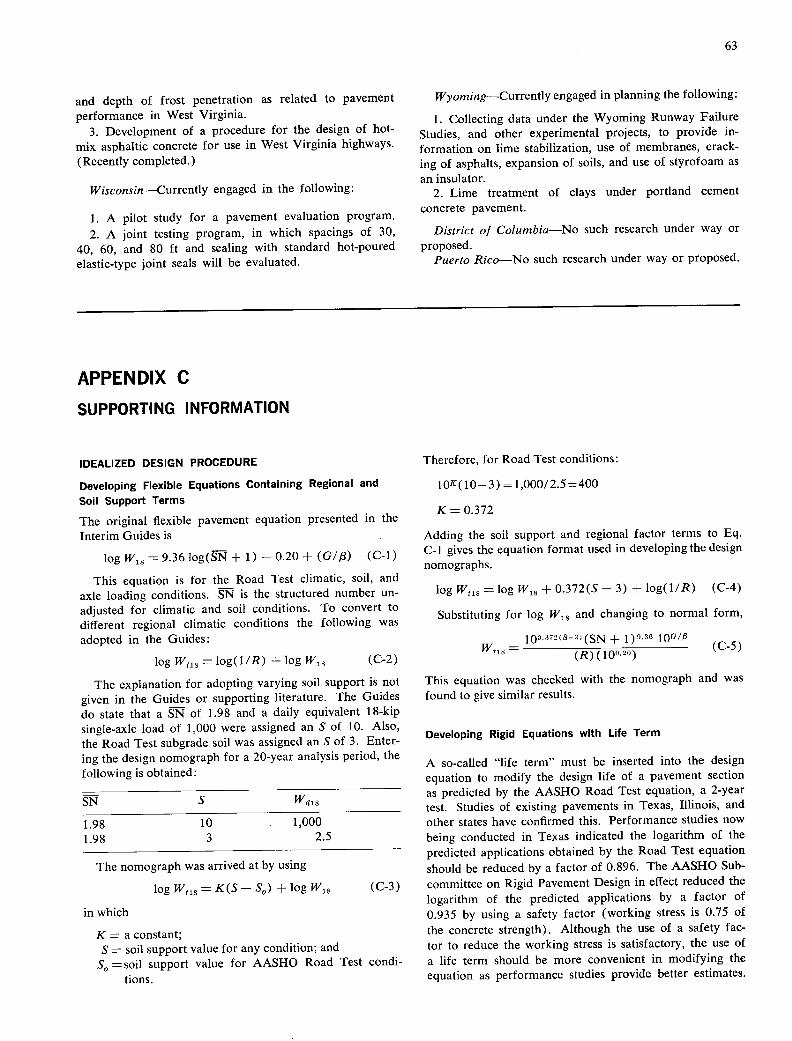
63

and depth of frost penetration as related to pavement performance in West Virginia.

3. Development of a procedure for the design of hot-mix asphaltic concrete for use in West Virginia highways. (Recently completed.)

Wisconsin—Currently engaged in the following:

1. A pilot study for a pavement evaluation program. 2. A joint testing program, in which spacings of 30,

40, 60, and 80 ft and sealing with standard hot-poured elastic-type joint seals will be evaluated.

Wyoming—Currently engaged in planning the following:

Collecting data under the Wyoming Runway Failure Studies, and other experimental projects, to provide in-formation on lime stabilization, use of membranes, crack-ing of asphalts, expansion of soils, and use of styrofoam as an insulator.

Lime treatment of clays under portland cement concrete pavement.

District of Columbia—No such research under way or proposed.

Puerto Rico—No such research under way or proposed.

APPENDIX C

SUPPORTING INFORMATION

IDEALIZED DESIGN PROCEDURE

Developing Flexible Equations Containing Regional and

Soil Support Terms

The original flexible pavement equation presented in the Interim Guides is

log W18 = 9.36 log(SN + 1) —0.20 + (G/$) (C-i)

This equation is for the Road Test climatic, soil, and axle loading conditions. SN is the structured number un-adjusted for climatic and soil conditions. To convert to different regional climatic conditions the following was adopted in the Guides:

log Wt18 = log (1/R) + log W18 (C-2)

The explanation for adopting varying soil support is not given in the Guides or supporting literature. The Guides do state that a SN of 1.98 and a daily equivalent 18-kip single-axle load of 1,000 were assigned an S of 10. Also, the Road Test subgrade soil was assigned an S of 3. Enter-ing the design nomograph for a 20-year analysis period, the following is obtained:

- S Wdls

1.98 10 1,000

1.98 3 2.5

The nomograph was arrived at by using

log W = K(S - S0 ) + log W18 (C-3)

in which

K = a constant; S = soil support value for any condition; and

S0 = soil support value for AASHO Road Test condi-tions.

Therefore, for Road Test conditions:

1OK(10_3) = 1,000/2.5=400

K = 0.372

Adding the soil support and regional factor terms to Eq. C-i gives the equation format used in developing the design nomographs.

log W 18 = log W1 + 0.372(S - 3) + log(i/R) (C-4)

Substituting for log W10 and changing to normal form,

10023'(SN + l0°/ Wtls = (C-5)

(R)(iO° 20 )

This equation was checked with the nomograph and was found to give similar results.

Developing Rigid Equations with Life Term

A so-called "life term" must be inserted into the design equation to modify the design life of a pavement section as predicted by the AASHO Road Test equation, a 2-year test. Studies of existing pavements in Texas, Illinois, and other states have confirmed this. Performance studies now being conducted in Texas indicated the logarithm of the predicted applications obtained by the Road Test equation should be reduced by a factor of 0.896. The AASHO Sub-committee on Rigid Pavement Design in effect reduced the logarithm of the predicted applications by a factor of 0.935 by using a safety factor (working stress is 0.75 of the concrete strength). Although the use of a safety fac-tor to reduce the working stress is satisfactory, the use of a life term should be more convenient in modifying the equation as performance studies provide better estimates.

64

In determining the magnitude of the life factor, the Interim Guides and the Texas performance studies were given equal consideration and an average factor of 0.9155 was selected. An extended version of the basic AASHO Road Test equation with a life factor applied has the following form (8):

\ log W 18 = —8.682 - 3.513 log sD2( 1 - 2.61a

Z¼ D%)

+0.9155G/ (C-6)

Only one term in Eq. C-6 has not been evaluated ade-quately—the continuity term J. The selection of a value for design purposes must still be on the basis of limited data. The value for the jointed pavements on the AASHO Road Test is automatically fixed at the value of 3.2, which was used in all correlation work. This value is assumed to apply to all jointed concrete pavements with adequate load transfer. A value of I = 2.2 is tentatively selected for continuously reinforced concrete pavement, based on comparative performance studies.

CONVERTING MIXED TRAFFIC TO

EQUIVALENT AXLE LOADS

The idealized concepts that should be included in any design procedure using the Guides appear in Chapter Ihree. One of these concepts was that an iterative process should be used in computing structural number of pave-ment thickness to ensure that the difference between the computed structural number and the assumed structural number is less than some predetermined tolerable value. Discussed in the following are:

The effect of structural number on pavement thick-ness, and of terminal serviceability on axle load equiva-lence factors.

The present procedures of the states for converting mixed traffic to equivalent axle loads for use in the design equations, and a comparison of each with the idealized design procedure.

The differences, in terms of component layer thick-nesses, between the ideal full iterative procedure and the semi-iterative process used by a number of agencies.

The mathematical models used to develop the load equivalence factors were derived from the AASHO Road Test data, and are of the following format.

For flexible pavements:

- (L+fl)4. 91r lOG/a 1

- [L + 1)4.79] [ 1o0/a(n)4.33] (C-7a)

For rigid pavements:

lOG/fl 1 e— [(L. + fl)l.621

- (L + 2][l0G/fl(n)7.2s] (C-7b)

in which

LL = the axle load being considered; and L = the axle load being used as a basis for equating

other axle loads.

The errors involved in using incorrect terminal service-ability terms or pavement dimensions are discussed in Chapter Three. The loadometer data used in the example comparison are given in Table C-i.

Several of the methods for converting loadometer data to equivalent wheel loading for design are compared in the following. Each procedure, with the exception of Method A, is being used by a highway department. Method A is the detailed procedure for converting mixed traffic that will give the greatest accuracy in predicting the equivalent axle load from the loadometer data as they are presently collected. Therefore, this method will be used as a basis for comparing the accuracy of the other methods in ap-plications under various traffic and wheel load distribu-tions. Methods B through G were derived for the condi-tions of a given state highway department, and, in most cases, certain assumptions were made in order to develop a procedure that could be put into use immediately. The basic assumptions for each of these methods and a brief description of each follow.

Method A

With Method A, the data presented in the W-4 loadometer forms used by most highway departments to report load-ometer data to the FHWA are used directly without change in grouping. In the W-4 tables, the axle loads are listed in groups that are generally in 2,000-lb increments. The number of axles in each group is then multiplied by the traffic equivalence factor for the average axle load for the group; e.g., for the 12,000- to 16,000-lb group, the traffic equivalence for a 14,000-lb axle load is used. This pro-cedure represents the most accurate use of the loadometer data in its present form; i.e., without classifying the axles into groups with smaller load ranges.

Method B

Method B is based on categorizing traffic into three basic classifications: passenger cars, single-unit vehicles, and multi-unit vehicles. A weighted equivalence factor for each vehicle type, based on the statewide average of vari-ous roadway classifications, is used to convert to equiva-lent axle loads. The equivalent axle load for each vehicle type is then distributed to the design lane. The basic equation is:

W 18 = DP (c1 PC P) + (c2 SU S) + (c3 MUM)

1,000,000 (C-8)

in which

DP = design period, years; C1 = constant for passenger cars;

= constant for single units; c3 = constant for multiple units;

PC = total passenger-car ADT (two directions) for the design period;

SU = total single-unit ADT (two directions) for the design period;

MU = total multiple-unit ADT (two directions) for the design period;

P = percent of passenger-car ADT in design lane;

65

S = percent of single-unit ADT in design lane; and M = percent of multiple-unit ADT in design lane.

The values of the constants c1, c.,, and C3 vary, depend-ing on pavement type and highway classification. The general classification used for the highway system is:

Class I—Roads and streets designed as four- (or more) lane facilities, or as part of a future four- (or more) lane facility.

Class TI—Roads and streets designed as a two- or three-lane facility with structural design traffic greater than 1,000 ADT.

Class Ill—Roads and streets with structural design traffic between 400 and 1,000 ADT.

Class IV—Roads and streets with structural design traffic less than 400 ADT.

The constants developed for rigid pavements to be used with Eq. C-8 are given in Table C-2. Only three highway classifications are given, because rigid pavements generally will not be used for a Class IV designation. Table C-3 gives the constants to be used with flexible pavements.

A basic limitation of this method is that, if the axle load distribution changes, the predicted traffic could be seri-ously in error. If this method is used by a state, the con-stants should be derived for that state, and on a yearly basis in order to assist in detecting trends.

Method C

Method C is almost identical to Method A, except that only ten axle groups (Table C-4) are used, compared to the 24 or more groups with Method A. An estimate is made of the total axles expected to use the facility in the future, and their distribution. As for Method A, a sum-mation is then made of the total equivalent 18-kip single-axle load applications. The result then is divided by 2 to give a 50/50 split of traffic by direction. The primary limitation of this method is that the group equivalence factors, as given in Table C-4, were developed on the basis of the average axle weight distributions for the state. Any change of axle distributions within the state would be reflected in an error for the total traffic predicted. A different set of load equivalence factors is used for flexible and rigid pavements.

Method D

Method D is similar to Methods A and C, except that a technique is used that enables the state to estimate future changes in axle load distributions. The general equation used for predicting total 18-kip single-axle loads is:

W 18 = (LDF) (DT) + (0.0002) (DPC) (C-9)

in which

LDF = load distribution factor; DTT = daily truck traffic or number of commercial

traffic; and DPC = daily passenger cars and light truck traffic.

By using the load distribution factor (LDF) term, the state predicts the change in the axle weight distribution

TABLE C-i

AVERAGE DAILY AXLE APPLICATIONS BY LOAD GROUPING ON A TYPICAL PRIMARY HIGHWAY

AXLE GROUPING NO. OF AXLES

(a) Single axles

Under 3000 0 3000-6999 337 7000-7999 278 8000-11999 762

12000-15999 121 16000-17999 101 18000-19999 181 20000-21999 173 22000-23999 64 24000-25999 11 26000-29999 5

(b) Tandem axles

Under 6000 1 6000-11999 203

12000-17999 181 18000-23999 93 24000-29999 133 30000-3 1999 85 32000-33999 106 34000-35999 93 36000-37999 57 38000-39999 35 40000-40999 12 41000-41999 5 42000-43999 6 44000-45999 3 46000-49999 1 1

TABLE C-2

RIGID PAVEMENT TRAFFIC CONSTANTS FOR METHOD B

TRAFFIC CONSTANTS

HIGHWAY PASS. SINGLE MULTIPLE

CLASS CARS UNITS UNITS

I 0.146 44.995 421.57 II 0.146 44.995 413.91

III 0.146 44.995 413.91

TABLE C-3

FLEXIBLE PAVEMENT TRAFFIC CONSTANTS FOR METHOD B

TRAFFIC CONSTANTS

HIGHWAY PASS. SINGLE MULTIPLE

CLASS. CARS UNITS UNITS

I 0.146 42.705 345.655 II 0.146 39.785 337.260

III 0.146 35.770 289.810 IV 0.146 9.855 78.840

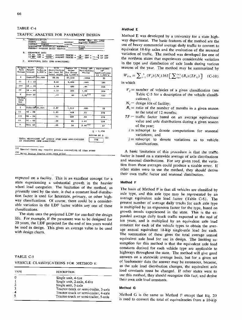
66

TABLE C-4

TRAFFIC ANALYSIS FOR PAVEMENT DESIGN IDENTIFICATION DATED Mar. 20, 1962 COUNTYName HIGHWAY Highway Number CONTROL Number LIMITS WADOMETER STATION(S) REFERENCE_L-cxx PRESENT AVERAGE DAILY TRAFFIC 1400

GEOMETRIC DATA 19 60 ADT = 1300 PERCENT TRUCKS = 18 DI!V S OF ADT 19= ADT = 20G, PERCENT TRUCKS = TE, DHV •% OF ADT

STRUCTURAL DATA (TWO DIRECTIONS)

STSjTh Axle

Groups

3XT0 Weight Groups

I'STST Axlexlo 1,000's

Axle Distributjox Per Cest Of TotalAxles

Number 01 Axles

Per Group is1,000's

Group 18s Equivalexcy

Factor __________

Equivalest l8I

Applications ix1,000's

I Usder5k 31,025 82.64 21,639 .0008 21

II 5 - 12 8.40 2,606 .069 180

III 12 - 16 1.58 490 .46 225

IV 16 - 20 1.13 351 1.02 358

V Over 20 .13 40 3.06(1) 122

Axle Set

Groups

I Under18 31,025 3.27 1,014 .023 23

II 18 - 28 1.83 168 .31 176

III 28 - 34 . 71 220 .81 178

IV 34 - 40 .26 81 1.4 1 114

Over 40 - .05 F 16 3.66(1) 1 57

5 - 1,456

DIVIDE BY 2

TOTAL 0UIVALENT 18' SINGLE AXLE LOAD APPLICATIONS {_728 1 (2)

IN THOUSANDS (ONE DIRECTION)

Special Cases may require precise evaluaio9 91 this group

(2) Ester Desigs Charts with this value.

expected on a facility. This is an excellent concept for a state experiencing a substantial growth in the heavier wheel load categories. The limitation of the method, as presently used by the state, is that a constant load distribu-tion factor is used for Interstate, primary, or other high-way classifications. Of course, there could be a consider-able variation in the LDF factor within any one of these classifications.

The state uses the projected LDF for one-half the design life. For example, if the pavement was to be designed for 20 years, the LDF projected for the end of ten years would be used in design. This gives an average value to be used with design charts.

TABLE C-5

VEHICLE CLASSIFICATIONS FOR METHOD E

TYPE DESCRIPTION

0 Single unit, 4-tire Single unit, 2-axle, 6-tire

2 Single unit, 3-axle 3 Tractor-truck or semi-trailer, 3-axle 4 Tractor-truck or semi-trailer, 4-axle 5 Tractor-truck or semi-trailer, 5-axle

Method E

Method E was developed by a university for a state high-way department. The basic features of the method are the use of heavy commercial average daily traffic to convert to equivalent 1 8-kip axles and the evaluation of the seasonal variation of traffic. The method was developed for one of the northern states that experiences considerable variation in the type and distribution of axle loads during various seasons of the year. The method may be summarized by

W8 = ( Vi) (N)3651 (Ri) (TF)] (C-b)

in which

V = number of vehicles of a given classification (see Table C-5 for a description of the vehicle classifi-cations);

N = design life of facility; R= ratio of the number of months in a given season

to the total of 12 months; IF = traffic factor based on an average equivalence

value and axle distributions during a given season of the year;

= subscript to denote computations for seasonal variations; and

j = subscript to denote variations as to vehicle classifications.

A basic limitation of this procedure is that the traffic factor is based on a statewide average of axle distributions and seasonal distributions. For any given road, the varia-tion from these averages could produce a sizable error. If other states were to use the method, they should derive their own traffic factor and seasonal distribution.

Method F

The basis of Method F is that all vehicles are classified by axle type, and this axle type may be represented by an average equivalent axle load factor (Table C-6). The present number of average daily trucks for each axle type is multiplied by an expansion factor for the type, based on growth trends experienced in the state. This is the ex-panded average daily truck traffic expected at the end of ten years, and is multiplied by an equivalent axle load constant for each of the vehicle types to obtain the aver-age annual equivalent 18-kip single-axle load for each. The summation of these gives the total average annual equivalent axle load for use in design. The limiting as-sumption for this method is that the equivalent axle load constants derived for each vehicle type are applicable to highways throughout the state. The method will give good answers on a statewide average basis, but for a given set of loadometer data the answer may be erroneous, because, as the axle load distribution changes, the equivalent axle load constants must be changed. If other states were to use this method, they should recognize this fact, and derive their own axle load constants.

Method G

Method G is the same as Method F except that Eq. 20 is used to convert the total of equivalencies from a lO-kip

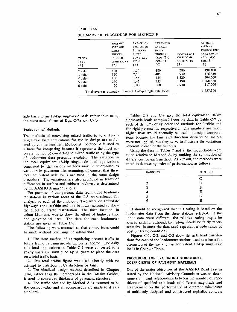
67

TABLE C-6

SUMMARY OF PROCEDURE FOR METHOD F

PRESENT EXPANSION EXPANDED AVERAGE

AVERAGE FACTOR TO AVERAGE ANNUAL

DAILY 10 YEARS DAILY EQUIVALENT

TRUCKS AFTER TRUCKS EQUIVALENT AXLE LOADS

TRUCK IN BOTH CONSTRUC- (COL. 2 X AXLE LOAD (C0L. 4 x TYPE DIRECTIONS TION COL. 3) CONSTANTS COL. 5)

(1) (2) (3) (4) (5) (6)

2 axle 400 1.70 680 280 190,400 3 axle 150 2.70 405 930 376,650 4 axle 100 1.55 155 1,320 204,600 5 axle 230 1.45 335 3,190 1,068,650

6 axle 60 1.00 60 1,950 117,000

Total average annual equivalent 18-kip single-axle loads 1,957,300

axle basis to an 18-kip single-axle basis rather than using the more exact forms of Eqs. C-7a and C-7b.

Evaluation of Methods

The methods of converting mixed traffic to total 18-kip single-axle load applications for use in design are evalu-ated by comparison with Method A. Method A is used as a basis for comparing because it represents the most ac-curate method of converting to mixed traffic using the type of loadometer data presently available. The variation in the total equivalent 18-kip single-axle load applications computed by the various methods may be interpreted as variation in pavement life, assuming, of course, that these total equivalent axle loads are used in the same design procedure. The variations are also presented in terms of differences in surface and subbase thickness as determined by the AASHO design equations.

For purpose of comparison, data from three loadome-ter stations in various areas of the U.S. were selected for analysis by each of the methods. Two were on Interstate highways (one in Ohio and one in Iowa) selected to show the effect of traffic distribution. The third location, in urban Montana, was to show the effect of highway type and geographical area. The data for each loadometer station are given in Table C-7.

The following were assumed so that comparisons could be made without confusing the interactions:

The state method of extrapolating present traffic to future traffic by using growth factors is ignored. The daily axle load applications in Table C-7 were converted to a yearly basis and multiplied by 20 years to place the data on a total traffic basis.

This total traffic figure was used directly with no attempt to distribute it by direction or lane.

The idealized design method described in Chapter Two, rather than the nomographs in the Interim Guides, is used to convert to thickness of pavement structure.

The traffic obtained by Method A is assumed to be the correct value and all comparisons are made to it as a standard.

Tables C-8 and C-9 give the total equivalent 18-kip single-axle loads computed from the data in Table C-7 by each of the previously described methods for flexible and for rigid pavements, respectively. The numbers are much higher than would normally be used in design computa-tions because the lane and direction distribution factors were not applied, but they serve to illustrate the variations inherent in each of the methods.

Using the data in Tables 7 and 8, the six methods were rated relative to Method A, by ranking the summation of differences for each method. As a result, the methods were rated in decreasing order of performance, as follows:

RANKING METHOD

1 C 2 D 3 F 4 E 5 G 6 B

It should be recognized that this rating is based on the loadometer data from the three stations selected. If the input data were different, the relative rating might be altered slightly, although the rating should be fairly repre-sentative, because the data used represent a wide range of possible traffic conditions.

Figures C-i, C-2, and C-3 show the axle load distribu-tions for each of the loadometer stations used as a basis for discussion of the variation in equivalent 18-kip single-axle loads in Chapter Three.

PROCEDURE FOR EVALUATING STRUCTURAL

COEFFICIENTS OF PAVEMENT MATERIALS

One of the major objectives of the AASHO Road Test as stated by the National Advisory Committee was to deter-mine significant relationships between the number of repe-titions of specified axle loads of different magnitude and arrangement on the performance of different thicknesses of uniformly designed and constructed asphaltic concrete

68

TABLE C-7

LOADOMETER DATA USED FOR COMPARING METHODS OF CONVERTING MIXED TRAFFIC

NUMBER OF AXLES

URBAN, INTERSTATE, INTERSTATE,

AXLE GROUPING MONTANA OHIO IOWA

(a) Single axles

Under 3000 2619 2498 512 3000-6999 569 5258 536 7000-7999 31 1853 239 8000-11999 85 8662 1453

12000-15999 25 2495 279 16000-18000 1823 106 16000-17999 13 18001-19000 856 1800 1-20000 43 18000-19999 4 1900 1-20000 548 20000-2 1999 0 20001-21999 534 4 22000-23999 0 368 3 24000-25999 0 94 0 26000-29999 0 15 0 30000-34999 0 0 0

Total axles counted 3346 25004 3175

(b) Tandem axles

TABLE C-8

COMPARISON OF VARIOUS METHODS OF CONVERTING MIXED TRAFFIC TO 18-KIP SINGLE-AXLE LOAD, FLEXIBLE PAVEMENTS (pt=2.S)

METHOD

TRAFFIC DATA FROM

URBAN, INTERSTATE, MONTANA OHIO

INTERSTATE,

IOWA

A 725,839 24,393,315 17,918,799 B 1,652,099 15,354,795 11,359,289 C 619,777 24,023,570 13,269,429 D 771,441 24,294,515 19,708,831 E 1,201,872 11,770,812 8,526,546 F 358,493 8,750,508 7,901,676 G 508,259 12,401,716 11,198,703

TABLE C-9

COMPARISON OF VARIOUS METHODS OF CONVERTING MIXED TRAFFIC TO 18-KIP SINGLE-AXLE LOAD, RIGID PAVEMENTS (p,=2.5)

TRAFFIC DATA FROM

URBAN, INTERSTATE, INTERSTATE, METHOD MONTANA OHIO IOWA

8 715 2 396 173 0 117 71 0 94 9 0 32 0 0 0 1 0 8 0 0 0 0 0 0 0

82 10246 2853

0 8 9 A 558,332 26,112,721 17,146,995 26 1564 337 B 1,902,882 28,297,272 13,899,330 11 1684 396 C 649,773 28,306,170 19,041,875 16 1772 457 E 1,582,056 16,457,339 11,921,374 13 2925 815 F 358,493 8,750,508 7,901,676

723 G 508,259 12,401,716 11,198,703 6

208 342 243

surfaces on different thicknesses of bases and subbases with a basement soil of a known characteristic. To accomplish this objective, a factorial design (45, Table 2), was set up to study the effect of different loads on similar and dif-ferent pavement structures. In addition to the main fac-torial design, two additional special experiments were in-cluded in loops 3 through 6. The first involved a study of pavement shoulders, and the second involved a study of the type of base material, which is of concern here. Four different types of base course material were used: crushed stone, gravel, cement-treated gravel, and bituminous-treated gravel.

On the basis of the results of this study, the AASHO Committee on Design evaluated the Road Test findings and established structural coefficients for the different types of materials used. These structural coefficients were in-cluded in the Interim Guide for design of flexible pave-ments and are summarized in Table C-b. The values established at the Road Test are marked with an asterisk; the remaining factors were estimated from the results of the special base study at the AASHO Road Test or through engineering and judgment factors. The constant values for structural coefficients in this table are a problem to pave-ment designers because they were established for the ma-terials used in the Road Test and are not necessarily ap-plicable to other paving materials. Consideration should be given to varying the structural coefficients as a function of material type or material properties. This point was made in the foreword to the Interim Guide for design of flexible pavements, where it was stated that ". . . careful consideration must be given by the user to those coefficients not established in the Road Test."

Study needed to fill the gaps in knowledge on structural coefficients may fall into four categories: (1) theoretical studies, (2) major satellite studies, (3) field tests, and 4) laboratory tests. As stated in HRB Special Report

Under 6000 6000-11999

12000-17999 18000-23999 24000-29999 30000-31500 30000-31999 31501-31999 30000-32000 32001-32999 32000-3 3999 34000-35999 3 6000-37999 38000-39999 40000-41999 42000-43999 44000-45999 46000-49999 50000-53999

Total axles counted

100

80

60

40

20

0

K, PS

Figure C-I. Axle-load distribution for the Montana loadometer station.

100

80

60

40

20

0 4 8 12 16 20 24 28

K,ps

Figure C-2. Axle-load distribution for the iowa loadometer station.

- 0 4 8 12 16 20 24 28 32 28 40

K,ps

Figure C-3. Axle-load distribution for the Ohio loadometer station.

40

69

70

TABLE C-b

EXTRACTS FROM TABLE 1, "AASHO INTERIM GUIDE FOR DESIGN OF FLEXIBLE PAVEMENT STRUCTURES"

COEFFICIENT

PAVEMENT COMPONENT a1 a, a

Surface course: Road mix (low stability) 0.20 Plant mix (high stability) 0.44 * Sand asphalt 0.40

Base course: Sandy gravel 0.07 Crushed stone 0.14 Cement treated (no soil-

cement) 650 psi or more' 0.231 400-650 psi 0.20 400 psi orless 0.15

Bituminous treated Coarse graded 0.34 Sand asphalt 0.30

Lime treated 0.15-0.30 Subbase:

Sandy gravel 0.11 * Sand or sandy clay 0.05-0.10

Compressive strength at 7 days. b This value has been estimated from AASHO Road Test data, but

not to the accuracy of those factors marked with an asterisk. It is expected that each state will study these coefficients and make such

changes as their experience indicates necessary.

61-E (45): ". . . [O]nly through such theoretical work will there be developed rational mathematical models by which performance can be related to the fundamental properties of materials and to dynamic characteristics of loading."

Following is a brief outline of the development of the AASHO Road Test coefficients, and a summary of pro-cedures currently used by a selected group of states and other agencies concerned with pavement design.

Development of AASHO Road Test Coefficients

In 1962, Liddle (61) outlined the methods used by the AASHO Committee on Design to apply the results of the AASHO Road Test to flexible pavement design. Liddle presented a method of determining layer thickness from structural number (SN). The relationship is expressed by

SN = a1 D1 + a, D, + a3 D. (C-il)

in which

a1, a,, as = coefficients of relative strength; = thickness of bituminous surface course,

inches; D2 = thickness of base course, inches; and D3 = thickness of subbase, inches.

The AASHO Road Test established coefficients for the types of surface course, base course, and subbase course used on the project. Coefficients used for other types of

materials were established by rationalization and a study of comparative cohesion, stability, and bearing values ob-tained in the laboratory. It should be noted that Liddle emphasized that further experience and research would be necessary to establish valid coefficients for all materials.

Selected Current Procedures for Determining Structural Coefficients

Arizona

Initially Arizona adopted the structural coefficient values established by the AASHO Road Test. Using these values as a guide, they established values for construction ma-terials used in Arizona. However, after using the estab-lished structural coefficient values in the design equation in evaluating the pavement structure for several projects, Arizona determined that the coefficients should be revised.

After considerable study and research,-these structural coefficients were revised and, in most cases, lower co-efficients were established. The ranges of the structural coefficients for each material used in Arizona are:

MATERIAL STRUCTURAL COEFFICIENT

Asphaltic concrete 0.34 to 0.42 Bituminous road mix 0.25 to 0.37 Bituminous-treated base 0.30 to 0.35 Cement-treated base 0.15 to 0.29 Aggregate base 0.08 to 0.14 Select material 0.05 to 0.12

The methods actually used to arrive at structural co-efficients for a material are summarized in Tables C-il and C-12. For example, in the case of select material, assume that the following conditions exist:

A non-plastic material. 0 to 10 percent passing the No. 200 sieve. 75 percent passing the No. 8 sieve. Crushed material passing the 3-in, slot.

The structural coefficient for this would be determined by adding the following to the base value 0.05: 0.01 for non-plastic materials, 0.02 for the percentage passing No. 200, 0.01 for percentage passing No. 8, and 0.01 for material crushed to pass the 3-in, slot. The resulting value of 0.10 would be the structural coefficient for this par-ticular select material.

Coefficients for aggregate base, bituminous-treated base, and asphaltic concrete are determined in a similar manner using the criteria given in Tables C-li and C-12.

The Asphalt institute

Shook and Finn (62) showed that the structural com-ponents (surfacing, base, and subbases) could be treated as linear combinations of equivalent thickness of each layer (D = a1 D1 + a, D, + a3 D3). Further, it was con-cluded that 1 in. of asphaltic concrete surfacing or asphalt base is equal to 2 in. of good crushed stone or 2.67 in. of subbase.

The method for determining these equivalence factors was based on an extensive survey of prior performance,

71

TABLE C-il METHODS USED TO ARRIVE AT STRUCTURAL COEFFICIENTS FOR A MATERIAL

SELECT MATER I AL

(STANDARD SPECS. - MAX. 5 P.1. WITH 251 PASS 200 OR MAX. 10 P.J. WITH 12% PASS 200)

fl ,n S & S. USE BASE COEFFICIENT Of

STRUCTURAL P. I. PASS 200 PASS 8 PASS CRUSHED

PASS 3 SLoT CRUSHED

PASS 3 COEFFICIENT

.01 N.P.

.01 0-15

.02 *0_10

.01 30-75

.02 30-75

100 .01 ____________

100 .02 ____________

*BAIED ON PIT INFOATION RATHER THAN SPECIFICATIONS.

A G G R E G A T E BASE

4lar •ar COEFFICIENT OF .08 FOR $ & C. USE BASE COEFFICIENT OF .06 FOR CINDERS.

STRUCTURAL P. I. — COEFFICIENT

PASS 200 PASS ASRASION CRUSHING

.02 N.P.

.00 0-12

.00 0-10

.01

.01 45-75

.01 _______________ _______________ <40

.01 _______________ 35% RET. j SIEVE

BASCD ON PIT INFOATION RATHER THAN SPECIFICATIONS.

including the results of the AASHO Road Test and the WASHO Road Test, together with theoretical considera-tions detailed by Skok and Finn (64). HRB Special Report

61-E (45) included a development of structural coefficients based on present serviceability index, Class 2 cracking, and deflection. On the basis of this analysis, Skok and Finn concluded that asphaltic concrete can be from two to six times as effective as good crushed stone. Other analy-ses of the same data (Klinger and Ferguson) indicated that the effectiveness of asphaltic concrete relative to good crushed stone was about 3.

As a result of these analyses, Shook and Finn performed three separate multiple linear regression analyses on the AASHO Road Test data, using the following models:

SN = 2.0 D1 + D2 + 0.75 D3 (C-12)

SN = 2.5 D1 + D, + 0.75 D3 (C-13)

SN = 3.0 D1 + D2 + 0.75 D3 (C-14)

The study was made to determine which coefficient gave the lowest error in the regression analyses. From this analysis it was concluded that any of the transformations for SN would fit the data with approximately the same error. Consequently, these investigators concluded that 1 in. of a high-quality asphaltic concrete surfacing should

be equivalent to 2 to 3 in. of good dense-graded crushed stone base, whereas asphaltic concrete base would be approximately equivalent to 2 in. of such crushed stone.

A theoretical investigation using layered elastic theory to interpret the AASHO Road Test data (64) suggests that when one is comparing vertical pressures on the subgrade it appears reasonable to use an equivalence factor of at least 2 to 1. Therefore, on the basis of the performance studies and theoretical studies, The Asphalt Institute de-cided on an equivalence factor of 2 to 1 for asphaltic concrete surface or base to aggregate base and 2.67 to 1 for asphaltic concrete surface or base to aggregate subbase.

California

Hveem and Sherman (14) give the California procedure for estimating gravel equivalencies of different construc-tion materials.

As a result of the performance of thicker asphalt sec-tions on the AASHO Road Test, the cohesion value scale in the California procedure was revised. Although the original formula assumed a cohesion of 100 for gravel and that no materials would be less than 100, it was evident that the gravel base used in the AASHO Road Test had a cohesion value of far less than 100. Tests performed on this material indicated a cohesion of only 20, and, for the

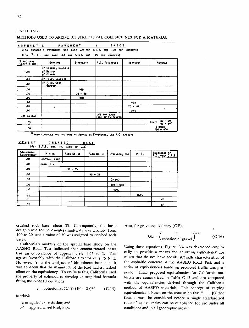
72

TABLE C-12

METHODS USED TO ARRIVE AT STRUCTURAL COEFFICIENTS FOR A MATERIAL

A S P H A L T IC PAVEMENT & 8 A S E S

(FOR ASPHALTIC PAVDIENTS USE BASE .25 FOR S & G AND .20 FOR CINDERS)

(FOR *B T B USE BASE .20 FOR S & G AND .15 FOR CINDERS)

STRUCTURAl. COEFFICIENT GRADING STABILITY A.C. IHICKNESS AsRASION ASPHALT

.02 COARSE, CLASS A MID

" COARI(MU

.Ci " FINE, CLASS B

.00 " FINE, OPEN GRADLD

.02 >35

.01 28-35

.00 428

.02

.01 25-40

.00 >40

.01 TO 0.8 .01 FOR EACH INCH SF THIcXNESS

.05 PENCT. :

.00 LIQUID 250-800

*WHEN CONTROLS ARE THE SANE AS ASPHALTIC PAVDIENT$, USE A.C. FACTORS

C E M E N T TREATED BASE (FOR C.T.B. USE THE BASE or .12)

STRUCTUAL. RCOEFFICIENT MIXING PASS No. 8 Pass No. 4 STRENGTH, PSI P. I. A.0

TNICXNESS OF . OVER C.T.B.

.05 CENTRAL PLANT

.00 ROAD MIX

.01 30-65

.02 45-75

.07 >500

.05 300-500

.00 <300

.01 N.P.

.01 4"

.02 6"

crushed rock base, about 33. Consequently, the basic design value for cohesionless materials was changed from 100 to 20, and a value of 30 was assigned to crushed rock bases.

California's analysis of the special base study on the AASHO Road Test indicated that cement-treated bases had an equivalence of approximately 1.65 to 1. This agrees favorably with the California factor of 1.75 to 1. However, from the analyses of bituminous base data it was apparent that the magnitude of the load had a marked effect on the equivalency. To evaluate this, California used the property of cohesion to develop an empirical formula fitting the AASHO equations:

c = cohesion at 72°[8/(W + 2)]2.5 (C-15)

in which

c = equivalent cohesion; and W = applied wheel load, kips.

Also, for gravel equivalency (GE),

GE = (

cohesion f gravel)° (C-16)

Using these equations, Figure C-4 was developed empiri-cally to provide a means for adjusting equivalency for mixes that do not have tensile strength characteristics of the asphaltic concrete at the AASHO Road Test, and a series of equivalencies based on predicted traffic was pro-

posed. These proposed equivalencies for California ma-terials are summarized in Table C-13 and are compared with the equivalencies derived through the California method of AASHO materials. This concept of varying equivalencies is based on the conclusion that ". . . [O]ther factors must be considered before a single standardized ratio of equivalencies can be established for use under all conditions and in all geographic areas."

CT• cT .

AAS A.C. CT

CT 2000

C. 1000

-\

CDLI,. A.C.

• - E,rEcTuvt COHESION, c - c1

(54)2.5

WHERE C, - COHESIONCTER VALUE AT MEAN PAVOSENT TOIPERATURE

c1

0- 0 2 4 6 0 10 12

3.0

- - 2.0

0.5

0.1

0.4

73

TRArruc INDEX

Figure C-4. Gravel equivalent of bituminous pavement based on AASHO Road Test analyses.

Illinois

Illinois has modified the structural coefficients presented in the Interim Guides. These modifications were developed to account for differences in strength of pavement ma-terials, and are based on the premise that the value of a coefficient for a particular layer is not constant, but would vary with the strength of the material used in this layer. Relationships between coefficient and material strength, as measured by the State of Illinois test procedures, were established for surface, base, and subbase materials. Ex-perience with the material coefficients developed on the AASHO Road Test, together with results of tests con-ducted by the state, were used in establishing these relationships.

The coefficient for the surface course, a1, was correlated with Marshall stability values (Fig. C-5). The upper value of 0.44 represents the bituminous concrete used on the Road Test; the lowest point, the lowest stability road mix; and the intermediate point, the Illinois Division of High-ways bituminous sub-class I-il.

The relationship between the coefficient a2 and ma-terials strength has been developed for four general cate-gories of base: granular materials, bituminous-stabilized granular materials, portland cement-stabilized granular materials, and lime-stabilized granular materials. Figure C-6 shows the relationship developed between coefficients for granular base and CBR. The upper and lower limits represent the Road Test crushed-stone base material and the Road Test sand and gravel subbase material, respec-tively, when used as a base course.

The coefficient for bituminous-stabilized granular base

GRAVEL EQUIVALENCY (IN.)

TRAFFIC

INDEX AASHO CALIF.

ROAD CLASS RANGE MATERIAL MATERIAL

Heavy industrial 12 2.0 1.6 11 2.1 1.7

Heavy truck traffic 10 2.2 1.8 9 2.3 1.9

Medium truck traffic 8 2.4 2.0 7 2.6 2.1

Light truck traffic 6 2.8 2.3 Residential streets 5 3.0 2.5

4 3.0 2.5

course materials was considered to vary with Marshall stabilities (Fig. C-7). The upper point represents the bituminous-treated base on the Road Test; the intermediate point, the grade 11 gravel stabilized with either emulsified or liquid asphalts; and the lower point, the Road Test sand and gravel material without treatment.

The coefficient for portland cement-stabilized granular base course materials was assumed to vary with 7-day compressive strength (Fig. C-8). Here the upper point represents the Road Test cement-treated base; the lower point, the same sand and gravel material without cement stabilization; and the intermediate point, a material with the minimum compressive strength for adequate durability of a soil-cement base.

For lime-fly-ash-stabilized granular base course mate-rials, it was assumed that the coefficient varies with the 21-day compressive strength (Fig. C-9), because perform-

400 800 1200 1600 2000 2400

MARSHALL STABILITY , lb

Figure C-5. Coefficient of the surface course correlated with Marshall stability values.

TABLE C-13

PROPOSED EQUIVALENC1ES FOR BITUMINOUS MATERIALS (Thickness of Gravel Layer Required to Equal 1 In. of Asphaltic Concrete)

0.24

va 0.20 0

I— z 0.16

0.150

0.125

CY 0.100

I-

0.075

LLJ

0.050

0.025

0.28

0.24

0.20 C"

0

I- 0.16 Lu U Lu..

b 0.12 0 L)

0.08

004

I hhuhll I I II Li -

0.6 I I

P.C.C. BASE— - 1(2500

0.4 - - - z w

CEMENT TREATED-01 - fr"BASE (650 psi) - - / 0.2

0 <..S0IL_ CEMENT BASE - — U

74 (300 p) -

- 00 1000 2000 3000 - — 7—DAY COMPRESSIVE STRENGTH, psi

(MINIMUM FIELD STRENGTH)

0 I I 1 I 1 111 1 I I Iii 1 I

C.WV 400 600 800 1000

20 40 60 80 tOO 200 7-DAY COMPRESSIVE STRENGTH, psi

C B R VALUE Figure C-8. Coefficient for portland cement-stabilized base course materials vs 7-day com- pressive strength.

Figure C-6. Relationship developed between coefficients from granular base andCBR. 0.28 [I

0.!

0.4

(1

0.3

z Uj

U.

0.2 Uj

U

0.1

0

MARSHALL STABILITY , lb 0 100 200 300 400 500 600 700 800 900

Figure C-7. Coefficient for bituminous-stabilized granular base 21—DAY COMPRESSIVE STRENGTH .psi course materials vs Marshall stability.

Figure C-9. Coefficient for lime-flyash-stabjljzed granular base course materials vs 21-day compressive strength.

75

ance data for lime-treated base course materials were not available.

The coefficient for subbase material was correlated with CBR (Fig. C-b). The upper and lower points represent the sand and gravel subbase material used on the Road Test and the material representative of the sandy clay, respectively.

Louisiana

For design of flexible pavements, Louisiana uses the co-efficients for Louisiana materials summarized in Table C-14. The coefficient for surface course is shown to be a function of Marshall stability, whereas the coefficients of the untreated and lime-treated base and subbase courses are a function of the Texas triaxial value. Cement-stabilized base is shown to vary as a function of com-pressive strength, whereas the asphalt-stabilized base ma-terials vary as a function of the Marshall stability. Co-efficients used in the design of overlays for both bituminous concrete and portland cement concrete pavements also are given in the table.

National Crushed Stone Association

Nichols (71) reported on triaxial tests performed on a wide range of construction materials. Nichols determined a relationship between vertical pressure at failure for vari-ous confining lateral pressures for large triaxial specimens on five different materials: slag or stone, normal gravel, asphaltic concrete, clay-gravel, and sand. At a 2-psi lateral pressure, the following vertical pressures at failure are indicated: slag or stone, 58 psi; normal gravel, 35 psi; asphaltic concrete, 29 psi; clay-gravel, 20 psi; and sand, 17 psi. From these data it would appear that slag or stone would be stronger than any of the other materials at a confining pressure of 2 psi for this test. Unfortunately, Nichols does not indicate the failure criterion used to establish the vertical pressure.

In addition, Nichols established layer equivalencies, using normal gravel as a standard, by dividing the vertical pressure at failure for each material by that for the stan-dard gravel at given lateral pressures. Table C-is sum-marizes these layer equivalencies for stone, slag, asphaltic concrete, sand, and clay-gravel in terms of the standard gravel as 1.0. These figures indicate that stone is from 1.48 to 1.65 times as strong as the standard gravel, and that slag macadam is from 1.04 to 1.72 times as strong. Asphaltic concrete is only slightly better than gravel at the lowest lateral pressure, and at a lateral pressure of 4.0 psi only about two-thirds as strong.

On the basis of additional analysis of Road Test data, Nichols also concluded that the equivalencies or structural coefficients of the materials used on the Road Test could not be assigned a constant value. Under light wheel load-ings, the ratio of asphaltic concrete to crushed stone was shown to be greater than 2.2 to 1, but for the heaviest loads it was only 1.8 to 1, thus indicating that for given increases in test load magnitude the increase in thickness of asphaltic concrete base required is almost as great as the required increase in thickness of crushed stone.

TABLE C-14

PAVEMENT COEFFICIENTS FOR FLEXIBLE SECTION DESIGN, LOUISIANA

ITEM STRENGTH COEFFI-dENT

Surface Course Asphaltic concrete

Types 1, 2, and 4 BC and WC 1000+ 0.40 Types 3 WC 1800+ 0.44

BC 1500+ 0.43

Base Course Untreated:

Iron ore-Grade B 3.7- 0.06 Sand clay gravel-Grade A 3.3- 0.08 Sand clay gravel-Grade B 3.5- 0.07 Shell and sand shell 2- 0.13

Cement stabilized: Soil cement 300 psi+ 0.15 Iron ore-Grade B 300 psi-i- 0.15 Sand clay gravel-Grade B 500 psi+ 0.17 Shell and sand shell 900 psi-i- 0.23

Lime stabilized: Sand shell 1.0 0.14 Sand clay gravel-Grade B 2.0- 0.12 Iron ore-Grade B 2.2- 0.11

Asphalt stabilized: Hot-mix base course (Type 3) 1200+ 0.34

Subbase Course Lime-treated sand clay gravel-

Grade B 2.0- 0.14 Lime-treated sand shell 1.0 0.15 Shell and sand-shell 2.0- 0.14 Sand clay gravel-Grade B 3.5- 0.11 Iron ore-Grade B 3.7- 0.10 Lime-treated soil 3.5- 0.11 Suitable material-A-6 (P1=15-) - 0.04 Old gravel or shell roadbed (8-in.

thickness) - 0.11 Sand (R-value) 55+ 0.10

Coefficients for Bituminous Concrete Overlay Base course:

Bituminous concrete pavement New 0.40 Old 0.24

Portland cement concrete pavement New 0.50 Old, fair condition 0.40 Old, failed 0.20 Old, pumping 0.10

New Mexico

New Mexico also varies the structural coefficients of pave-ment components with strength. For the surface layers, New Mexico uses Figure C-li to vary the structural co-efficient as a function of Marshall stability. For untreated granular bases and subbases, Figure C-12 summarizes the variation in structural coefficient as a function of R-value. In both cases, these correlations with strength parameters were provided by the FHWA, Denver Region.

76

0.150

0.125

0.100

I— z LLJ 0.075

0.050

0.025

0 • II I I I I I I liii

2 4 6 8 10 20 40 60 80 100

C B R VALUE

Figure C-JO. Coefficie,zt for subbase material vs CBR value.

50

Based on Graph rurnished by the FHWA, Denver Region.

1000 1100 1200 1300 1400 1500 1600 1700 1800 1900 2000 MARSHALL STABILITY, POUNDS

Figure C-li. chart for estimating structural coefficients of bituminous pavement mixtures based on Marshall stability, New Mexico.

TABLE C-iS

STRENGTH INDICES RELATIVE TO STANDARD GRAVEL BASE ON TRIAXIAL TEST

STRENGTH INDEX, BY

LATERAL PRESSURE OF

MATERIAL 0.5 PSI

1.0 PSI

2.0 PSI

Stone 1.48 1.65 1.63 Slag 1.04 1.42 1.63 Asphaltic concrete 1.04 0.96 0.83 Sand 0.22 0.35 0.49 Clay-gravel 0.48 0.58 0.57

Source: Nichols (71).

Ohio

Coffman, et al. (67) developed a method for establishing equivalencies on a continuous basis for a 245-day period; that is, for determining a representative value that accounts for variations in stiffness during the period. For these

4.0 calculations, equivalence was defined as that thickness of

PSI base necessary to replace 1 in. of surfacing for equal de- flection. Deflections were calculated using layered elastic 1.60

1:72 theory, and the results of static and dynamic laboratory 0.68 tests of pavement materials in the frequency domain. The 0.64 materials investigated were two asphaltic concrete surfac- C)

ings (the AASHO Road Test surface and a typical Ohio surface) and three asphaltic concrete bases (the AASHO

77

90

I I I I I I

88 - COEFFICIENT = .14 - (.006 X 83 - RX) -

86 - XR_VALUE OF MATERIAL BEING COMPARED WITH - CRUSHED LIMESTONE AND SAND FILLER BASE

84 - USED ON AASHO ROAD TEST. -

Based on Graph furnished by the FHWA, 82 - Denver Region. -

uJ -j 80 >

78

76

74

72

70

I I I I I I I Ok .06 .08 .10 .12 .14 .16 .19 .21

STRUCTURAL COEFFICIENT

Figure C-12. Chart for estimating structural coefficients of granular subbase and base ma-terial based on stabilometer R-value, New Mexico.

Road Test asphaltic concrete base and two typical Ohio asphaltic concrete bases). The subgrade properties as-sumed were those determined from 1960 trenchings at the AASHO Road Test, and the continuous hourly tempera-ture data were those reported by The Asphalt Institute for the College Park, Md., location. Continuous 19-kip single-axle loadings, moving at 50 mph, were assumed for the principal calculations. These calculations resulted in the average equivalencies for a 245-day period summarized in Table C-16.

In addition to the primary analysis, several secondary analyses were made to determine the effects of different loadings as functions of weight, speed, time, and contact area, together with the effects of different subgrades and layer thicknesses. It was shown that changes in subgrade did not make a significant change in the layer equivalency,

whereas, for in-service pavements, vehicle speed can affect equivalencies significantly.

It was also shown that the layer equivalency is a func-tion of the thickness of the base layer. For the analysis reported, decreasing the base thickness by two-thirds re-sulted in roughly doubling the deflections and slightly decreasing the layer equivalence factor.

In summary, it was concluded that there is no unique equivalence factor, and that the inclusion of a failure term is necessary for theoretical calculations of equivalency for given materials, environment, and loading.

Texas

Tentative material coefficients to supplement the co-efficients provided in the Interim Guides were prepared wherever possible based on studies of AASHO Road Test

TABLE C-l6

245-DAY DATA, OHIO

AASHO SURF., AASHO SURF., T-35 SURF., T-35 SURF., T-35 SURF.,

ITEM AASHO BASE B-21 BASE u-35 BASE AASHO BASE B-21 BASE

(a) Equivalence (in.)

Average 1.24 1.28 0.78 0.83 0.90

High (4th hr) 1.53 1.51 1.03 1.05 1.06

Low (4th hr) 1.05 1.12 0.39 0.41 0.53

(b) Deflection (10 in.)

Average 16.5 16.9 18.5 18.9 19.5

High (4th hr) 23.7 23.2 31.7 31.3 30.7 Low (4th hr) 10.9 11.6 12.5 12.7 13.6

78

materials. Certain coefficients were based on the collec-tive experience of several engineers throughout Texas. Coefficient ranges for the various materials are as follows:

Granular bases and subbases, untreated and lime-treated—Figure C- 13 shows a plot of structural coefficients versus triaxial class based on Road Test materials.

Asphalt-treated bases—Figure C-14 shows structural coefficients for asphalt-treated material as a function of the Texas triaxial class at 140°F.

Cement-treated bases—Figure C-15 shows the esti-mated variation in structural coefficient for cement-treated materials as a function of 7-day unconfined compressive strength.

Asphaltic concrete—Figure C-i 6 shows the best esti-mate available for the variation of coefficients with co-hesiometer value. This curve indicates advantages for asphaltic concrete with a cohesiometer value of around 200, but little added credit for higher cohesiometer values.

The foregoing coefficients are being checked against field performance throughout the state. A systematic correla-tion of a great many pavement sections is expected to allow the statistical study of isolated variables.

Wyoming

Wyoming uses an approach similar to that of New, Mexico for varying structural coefficients as a function of a strength parameter. For surface courses, Wyoming varies the structural coefficient as a function of Marshall stability.

This relationship is shown in Figure C-17. For granular subbase and base materials, the variation of structural coefficient with R-value is shown in Figure C-18.

DEVELOPMENT OF A RATIONAL SOIL SUPPORT SCALE

As mentioned in the Interim Guide for design of flexible pavements, many basic assumptions were made in the development of the design charts in the Guides. One of these assumptions was:

It has been necessary to assume a scale for the soil sup-port value on [the design] charts. . . . 3.0 on the scale represents the silty clay roadbed soils on the Road Test, it is a firm and valid point. 10.0 represents crushed rock base material such as used on the AASHO Road Test. It is a reasonably valid point. All other points on the scale are assumed.

Following is a discussion of the approach used to check the validity of the soil support scale for use in the design of flexible pavements.

The need for planned satellite studies subsequent to the Road Test was clearly emphasized in HRB Special Report 61-E (45), particularly from the standpoint of strengthen-ing the soil support scale. Satellite studies on soils differ-ing from those at the Road Test would make it possible to establish empirically a stronger based and a more reliable soil support scale. Because of the limited number of satel-lite studies that have been conducted, it was apparent that some other means must be used to strengthen the soil sup-port scale. One such means is through application of theory, such as layered elastic analysis.

Several investigators have established the applicability of

07-

0

05-

10 20 30 40

50 the

Texas Triaxial Soil Class (TEX-117-E)

Figure C-13. Granular bases and subbases, natural and lime-treated.

z

0

U

100 400 600 800 1000 1200 7 Day Unconfined Compressive Strength - PSI

Figure C-15. Cement-treated materials.

4

":''.....

A ninimun Hveem Stability value of 30 shall be provided

1.0 2.0 3.0 4.0 100 200 300

400

Texas Triaxial Class at 140° (TEX-121-E) Cohesiometer Valoe

Figure C-14. Asphalt-treated materials. Figure C-16. A sphaltic concrete.

I 34 -z 'U a

32

'a.

'U 0

30 —I 4 0 ,_ 28 a 0 I-

26

WA

layered elastic theory to the prediction of deflections and of stresses and strains in a pavement structure. These investigators have indicated the reliability of these pre-dicted responses through comparisons of measured re-sponses on either prototype pavements or full-scale test roads. On the basis of these investigations it was con-cluded that a first step toward a rational soil support scale should be the application of layered elastic theory, and that additional refinements should be made as new develop-ments and new methods for characterizing the pertinent properties of pavement components become available.

The response of the pavement to one dual wheel of an 18-kip axle load (i.e. two 4,500-lb wheel loads) is used for this analysis. The contact area for each of the loads is assumed to be circular, and the spacing between the tires is assumed to be equal to one load radius. The variables considered in this analysis are:

The modulus of the surface layer (E1), 150,000 and 600,000 psi.

The modulus of the base layer (E2), 15,000 psi. The modulus of the subgrade layer (E3), 3,000,

7,500 and 15,000 psi. The thickness of the surface layer (D1), 3, 4, 5, 6,

8, and lOin. The thickness of the base layer (D2).

The surface and base moduli, and one level of sub-grade modulus (E3 == 3,000 psi), are similar to that estab-lished at the AASHO Road Test. The other values of subgrade modulus, 7,500 and 15,000 psi, were selected primarily to represent a wide range of subgrades from poor to good, with assumed correlation with CBR values about as follows:

40

38

36

24

22

20 I 000

200 1400 1600 1800 2000 MARSHALL. STABILITY, POUNDS

Figure C-17. Chart for estimating structural coefficients of bituminous pavement mixtures based on Marshall stability, Wyoming.

SUBGRADE TYPE MODULUS (Psi) CBR

Poor 3,000 2 Fair 7,500 5 Good 15,000 10+

Also considered in the analysis were six levels of surface thickness, ranging from 3 to 10 in., to cover the broad

Iü 1

4 >

80

78

76 WI', I (04

210

T4 cr o I Z

I OW 721— 2 U)

cc

70

.02 .04 .06 .Ub .

STRUCTURAL COEFFICIENT

Figure C-18. Chart for esti,nating structural coefficients of granular subbase and base mate-rial based on stabilometer R-values, Wyoming.

80

range of surfacing thickness used on heavy-duty highways. The corresponding base thicknesses used for each surface level were determined from

SN = a1D1 + a2D2 (C-17)

in which SN is the structural number; a1 and a, are struc-tural coefficients for the surface and base, respectively; and D1 and D. are the thickness of the surface and base, respectively.

Several investigators have indicated that two of the most critical responses in the pavement are the tensile strain on the bottom fiber of the asphaltic concrete (Ea0) and the vertical compressive strain on the subgrade (E89). The first is generally associated with fatigue cracking, and the second is associated with distortion of the pavement, such as rutting or corrugating. For this analysis, E90 and E11, were calculated for each of the combinations of variables with the aid of an IBM 6400 digital computer and Chev-ron Research Corporation's program for solution of the layered elastic equation. Calculations were made for one 4,500-lb tire load, and, in order to obtain the effect of the dual tires, the response of a second 4,500-lb tire spaced at three load radii was superimposed on it. The results of the calculation are shown in Figures C-19 and C-20. Note that Eac and E9 are functions of the structural number, the subgrade modulus, and the surface modulus.

The values for equivalent 1 8-kip single-axle load ap-plications to a given level of serviceability were calculated using the following equation from the Interim Guides:

log W 1 =9.36log( N + 1) —0.20+ 0.40+ (

G 1094 ,

1)1.19

(C- 18)

For each structural number, unadjusted for climatic and soil conditions, the number of equivalent 18-kip single-axle load applications (W118 ) was calculated for terminal ser-viceability indices of 2.5 and 2.0, with results as follows:

EQUIVALENT 1 8-KIP SINGLE-AXLE

LOAD APPLICATIONS, W118

SN Pt2.5 Pt= 2'°

1.5 3,193 3,278 2.0 16,454 17,534 3.0 186,514 230,335 4.0 1,088,780 1,610,795 5.0 4,805,546 8,044,522 6.0 18,138,485 32,365,071

On the basis of the relationships established here, and the calculated strains summarized in Figures C-19 and C-20, Figures C-21, C-22, and C-23 were prepared to show the relationships of both vertical compressive strain and tensile strain in the bottom fiber of the asphaltic concrete as functions of W.18 for terminal serviceability indices of 2.5 and 2.0 for the AASHO Road Test conditions, and two levels of surface modulus (150,000 and 600,000 psi).

PROCEDURE FOR DETERMINING REGIONAL FACTORS

Over the years, many investigators have shown that en-vironment can significantly affect pavement performance. For example, a given pavement may perform well in an and region, but may have a short service life if constructed in a wet climate. One of the major weaknesses of the AASHO Road Test was that the design equations relating traffic load and repetitions to performance over a range of structural sections were established for one environment only. The AASHO Committee on Design included in the Interim Guide for design of flexible pavements a factor, which they called the regional factor (R). This factor permits an adjustment to be made in the structural num-ber to reflect climatic and environmental conditions differ-ing from those at the Road Test site. The method sug-gested in the Interim Guide for estimating a regional factor is based on the duration of certain typical conditions during an annual period. Based on this method, the values for certain typical conditions are given in Table C-17.

Summarized in the following are the procedures used by selected states for determining regional factors. The states were selected primarily because they provided a cross-section of procedures used throughout the U.S.

Arizona—divided into three zones on the basis of eleva-tion, as follows:

Zone 1: desert areas below 3,500 ft in elevation where the soils are considered to be dry all year. A regional factor of 0.5 to 1.0 is used.

Zone 2: intermediate areas, 3,500 to 6,000 ft eleva-tion, where soils are dry through all but the late winter and early spring months, subject to freezing temperatures but with only a minimum of frost damage. A regional fac-tor of 1.0 to 1.5 is used.

Zone 3: mountainous areas, above 6,000 ft elevation, in which saturated soils would be expected the major por-tion of the year, and where frost damage would be antici-pated. A regional factor of 1.5 to 3.0 is used.

Georgia—Figure C-24 shows the regional factors used. These regional factors were selected on the basis of judg-ment and experience for varying topography, rainfall, water table, and temperature. Higher regional factors are assigned to the northwestern portion of the state, where there are higher elevations and greater temperature variations.

Idaho—Idaho conducted an extensive study to determine the effect of climate and environment on the performance of flexible pavements. The following were considered in the development of their climatic or regional factors:

I. Road Test results—Both the AASHO and WASHO Road Test results were investigated with respect to the amount of distress during different seasons of the year.

Interim Guide regional factor—Using the procedure described in Appendix G of the Interim Guide, each dis-trict in the state established its own regional factors. Re-ports indicated that the correlation between districts and the conformity at district borders was good.

Idaho weather—Weather Bureau records were re-viewed, particularly with regard to duration of freezing

81

TABLE C-17

AASHO INTERIM GUIDE RECOMMENDATIONS FOR REGIONAL FACTOR

REGIONAL

PAVEMENT CONDITION

FACTOR (R)

Roadbed soil frozen (5-in, depth or more) 0.2 to 1.0 Roadbed soil dry (summer and fall) 0.3 to 1.5 Roadbed soil saturated (spring break-up) 4.0 to 5.0

weather and precipitation during winter months. Degree-day curves were drawn for each station (Fig. C-25). These data, together with a district maintenance engineer's evaluation of spring breakup periods, were used to estab-lish the map for climatic factors shown in Figure C-26. Note the similarity to the previous figure.

On using the Guides' recommendations for increasing pavement thickness in accordance with climatic conditions, the following procedure was developed for adjusting struc-tural thickness as a function of climate:

15000

3 x 103 7.5 x 10 15 x 10 3 x 103 7.5 x 103 15 x 103

1.5 .0011758 .0008289 .0006381 .0005585 .0004175 .0003314

-

SN

1.5

14.0 .0006290 .0006282 - .0006272 .0003578 .0003402 .0003287 3

3 22.3 .0006118 .0006212 .0006263 .0003357 .0003314 .0003283 4

30.7 .0006103 .0006205 - .0006261 .0003287 .0003285 .0003281 5

- 39.0 .0006112 .0006207 .0006259 .0003262 .0003275 .0003280 6

2.0 .0009054 .0006760 .0005458 .0004017 .0003133 .0002564 2

10.3 .0005883 .0005580 .0005397 .0003056 .0002753 .0002576 3

4 18.7 .0005402 .0005395 .0005358 .0002728 .0002627 .0002559 4

27.0 .0005303 .0005355 .0005380 .0002615 .0002581 .0002557 5

- 35.3 .0005281 .0005346 .0005378 .0002570 .0002562 .0002555 6

6.7 .0005671 .0004978 .0004577 .0002674 .0002288 .0002045 - 3

15.0 .0004774 .0004644 .0004559 ,0002294 .0002141 .0002039 4

5 23.3 .0004565 .0004561 .0004554 .0002146 .0002081 .0002037 5

31.7 .0004502 .0004536 .0004552 .0002081 .0002053 .0002036 6

3.0 .0005793 .0004595 .0003888 .0002350 .0001943 .0001663 3

11.3 .0004321 1.0004035 .0003859 .0001979 .0001784 .0001657 4

6 19.7 .0003963 .0003897 .0003851 .0001806 .0001714 .0001654 5

28.0 .0003852 .0003853 .0003848 .0001727 .0001682 .0001654 6

12.3 .0003180 .0002951 .0002808 .0001358 .0001226 .0001143 5

- 20.7 .0002931 .0002854 8 -

.0002803 .0001263 .0001187 .0001141 6

5.0 .0002856 .0002409 .0002122 .0001076 .0000926 1.0000828 5 10 - 13.3 .0002402 .0002224 .0002113 .0000986 1 .0000885 .0000827 1 6

Figure C-19. Summary of calculations for tensile strain in the bottom fiber of the asphaltic concrete (response due to both tires).

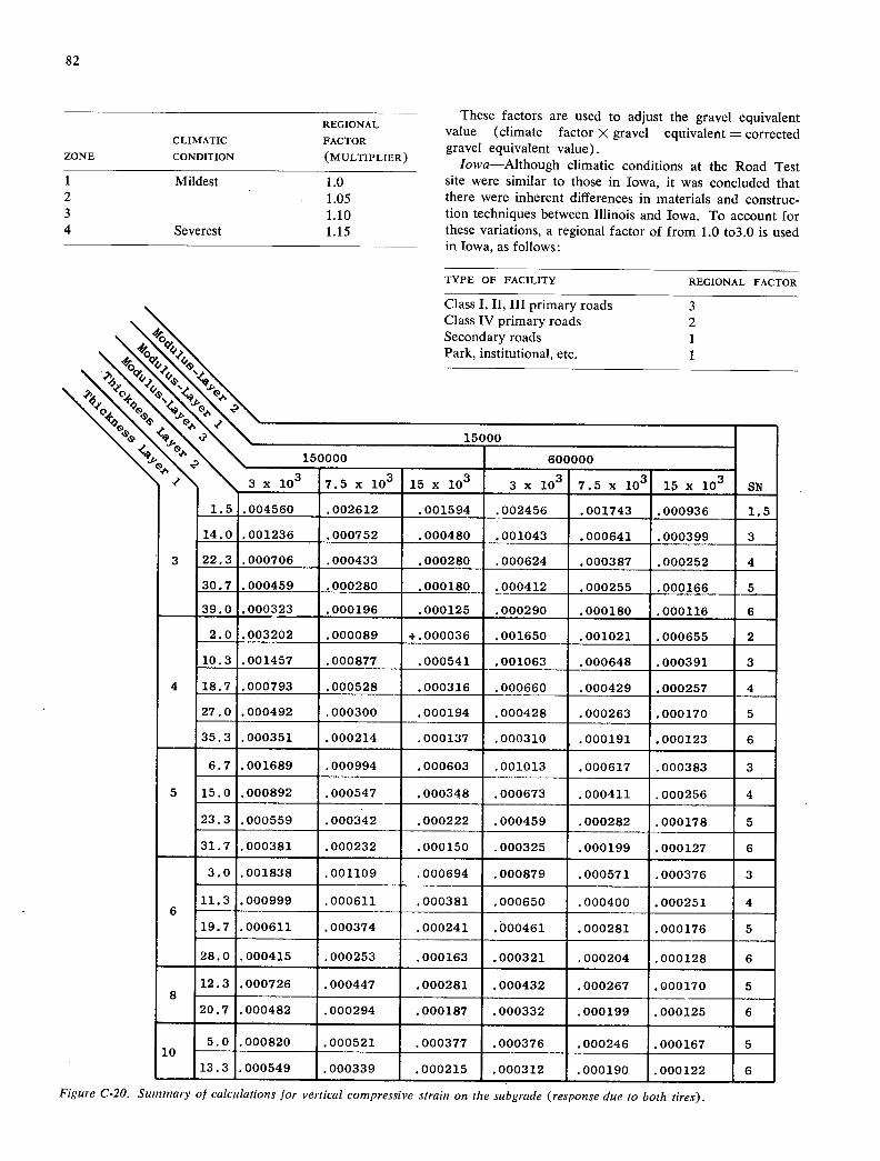
82

ZONE

1 2 3 4

CLIMATIC

CONDITION

Mildest

Severest

These factors are used to adjust the gravel equivalent REGIONAL

value (climate factor X gravel equivalent = corrected FACTOR

gravel equivalent value). (MULTIPLIER)

Iowa-Although climatic conditions at the Road Test 1.0 site were similar to those in Iowa, it was concluded that 1.05 there were inherent differences in materials and construc- 1.10 tion techniques between Illinois and Iowa. To account for 1.15 these variations, a regional factor of from 1.0 to3.0 is used

in Iowa, as follows:

TYPE OF FACILITY REGIONAL FACTOR

Class I, II, III primary roads 3 Class IV primary roads 2 Secondary roads 1 Park, institutional, etc. 1

\ '\ ' 15000

\0000 600000

/ 3x10 7.5x103 15x103 3x 10 7.5x103 15x103

1.5 .004560 .002612 .001594 .002456 .001743 .000936

-

SN

1.5

14.0 .001236 .000752 .000480 .001043 .000641 .000399 3

3 22.3 .000706 .000433 .000280 .000624 .000387 .000252 4

30.7 .000459 .000280 .000180 .000412 .000255 .000166 5

- 39.0 .000323 .000196 .000125 .000290 .000180 .000116 6

2.0 .003202 .000089 +.000036 .001650 .001021 .000655 2

10.3 .001457 .000877 .000541 .001063 .000648 .000391 3

4 18.7 .000793 .000528 - .000316 .000660 .000429 .000257 4

27.0 .000492 .000300 .000194 .000428 .000263 .000170 5

- 35.3 .000351 .000214 .000137 .000310 .000191 .000123 6

6.7 .001689 .000994 .000603 .001013 .000617 .000383 3

5 15.0 .000892 .000547_- .000348 .000673 .000411 .000256 4

23.3 .000559 .000342 .000222 .000459 .000282 .000178 5

- 31.7 .000381 .000232 .000150 .000325 .000199 .000127 6

3.0 .001838 .001109 .000694 .000879 .000571 .000376 3

6 11.3 .000999 .000611 .000381 .000650 .000400 .000251 4

19.7 .000611 .000374 .000241 .000461 .000281 .000176 5

- 28.0 .000415 .000253 .000163 .000321 .000204 .000128 6

12.3 .000726 .000447 .000281 .000432 .000267 .000170 5

20.7 .000482 .000294 .000187 .000332 .000199 .000125 6

5.0 .000820 .000521 .000377 .000376 .000246 .000167 5, 10

13.3 .000549 .000339 .000215 .000312 .000190 .000122 6

Figure C-20. Summary of calculations for vertical compressive strain on the subgrade (response due to both tires).

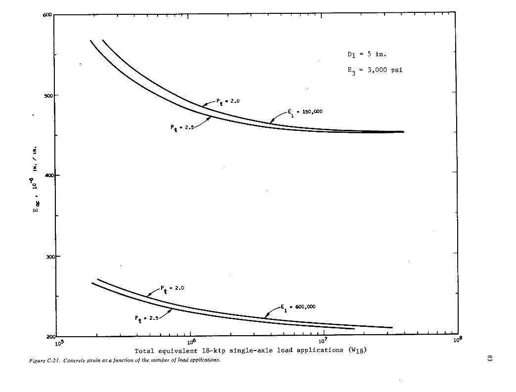
10 100 10' 10

Total equivalent 18-kip single-axle load applications (W18) 00

Figure C-21. Concrete strain as a function of the number of load applications.

Di = 6 in.

E1 = 150,000 psi

E3 = 3,000 psi

Pt 2

2.0

105 io6 107 to8

Total equivalent 18-kip single-axle load applications (W18) Figure C-22. Subgrade strain as a function of the number of load applications. E1 150,000 psi.

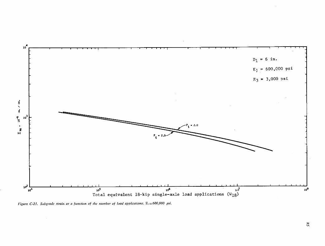
4 10

Dl = 6 in.

E1 = 600,000 psi

E3 = 3,000 psi

Pt

2.0

102L

105 106 icd

100

Total equivalent 18-kip single-axle load applications (W18)

Figure C-23. Subgrade strain as a junction Of the number of load applicat ions. E1= 600,000 psi.

00

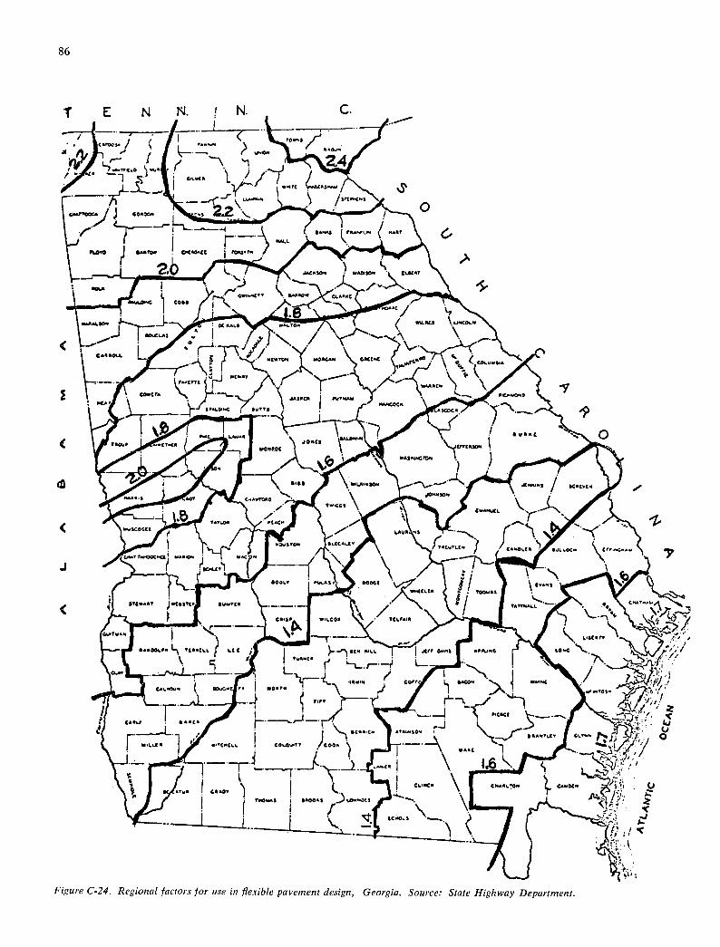
86

_tc L.,_

—7 0000. /

<7.___._l••

— 091.t

ovG 090?00 . 90631?" .

210 L. )

1 0N6C" ,06'b ._(t.800C

_6 -. •...j... 60t

6 • p.—. \

Cb_190

\spc.

l•9t60 09111 .

I / Swolac • town ( 10060 1Ln

tiQN90C •\ JONIS \I6

,tM0#

SIll 0L*IItlCn . / SCOEN

601 c..*oo L96'ntCi. '—i .-.ZT . ••..

( cot i...uo -. ( •\ 'l• / 0061106 S921 /'9C9,LC I ) ,ttoco

j I .

-TL •oot.0 901.60 00001 .

- ., WI.CLLCS . 1001.151

$i(w5? 59511(5

C \P

" WI1.006

1811061.1.

.1055 . t •_• — 5.•.

t,$(1 • 560601.0. I... 1(5 0C1. 1.1€ ...'1 9(N 51.1. 9oI9 •9.ING 1.060 \.

Co"

( 009001 1, welTs . . I.00 .,7 d,

.4 ,. I 01(5CC '(

'5L.. r------'•'-

\ 5(50,155 OTO,OOON r- "'" 1 ' • 601.011111 )Co..

5691

S 00 1 1.069000 \

•p.ij

ell

Figure C-24. Regional factors for use in flexible pavement design, Georgia. Source: State Highway Department.

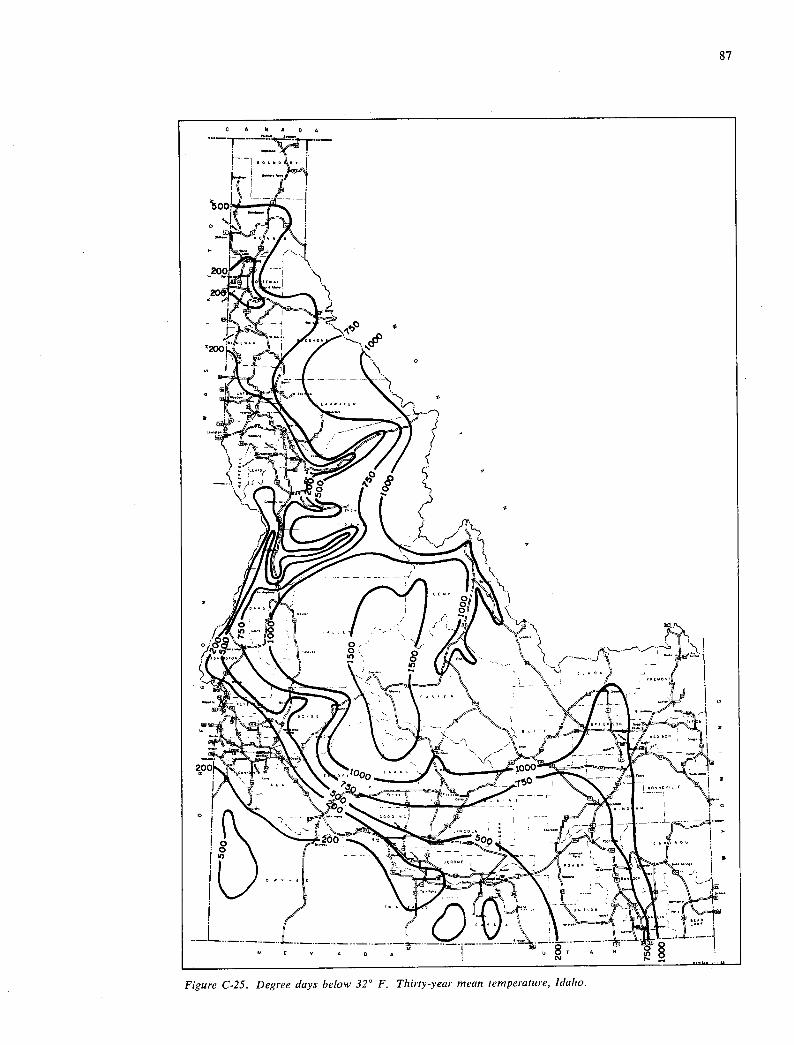
87

Figure C-25. Degree days below 32° F. Thirty-year mean temperature, Idaho.

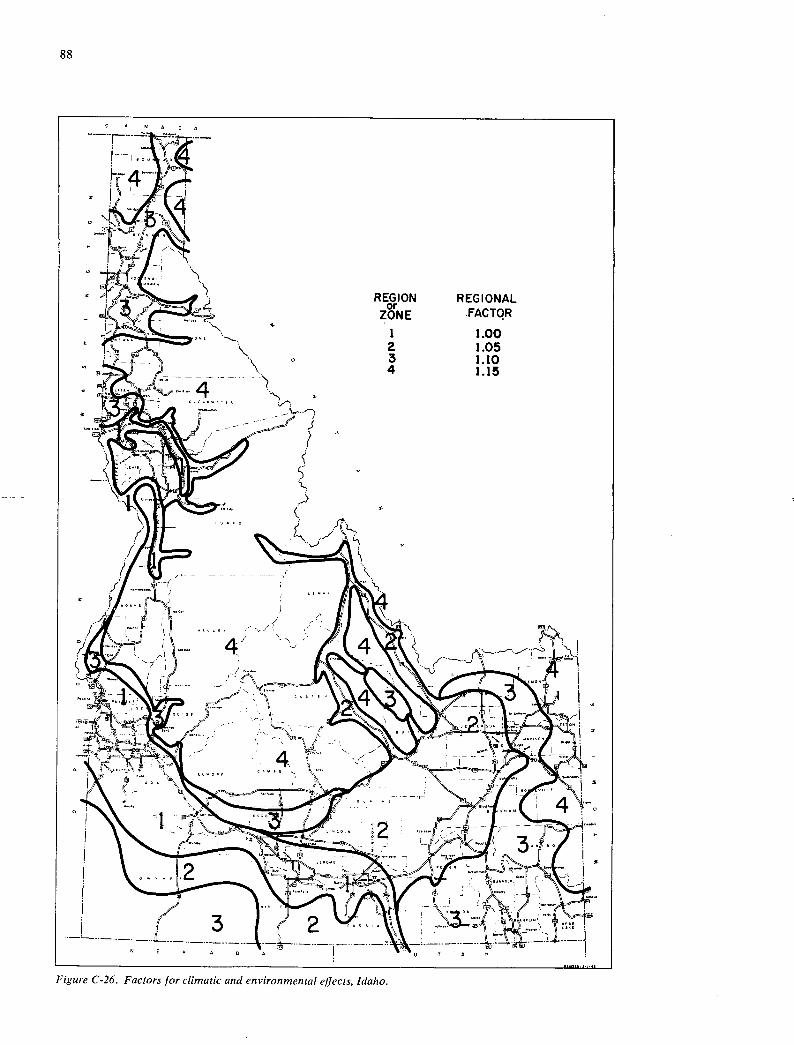
88

Figure C-26. Factors for climatic and environ,nental effects, Idaho.

89

It should be noted that these factors were established on the basis of level of service, rather than on area.

Nebraska—Nebraska considers not only level of service, but also subsurface drainage and average annual precipita-tion. These factors, developed on the basis of experience and engineering judgment, are selected by means of Fig-ure C-27. As indicated in this figure, considered are three levels of rainfall (light, medium, and heavy); four levels of drainage situation (ridges and good drainage, level, water table deep, and water table high); and a range of axle loading factors.

New Hampshire—Three regional factors are assigned within the state, as follows:

REGION REGIONAL FACTOR

Coast 2.0 Central 2.5 North 3.0

These factors were arrived at on the basis of engineering judgment and the number of degree-days within the region.

New Mexico—Regional factors are based on variations in climatic conditions, as follows:

Roadbed soil frozen to a depth of 5 in. or more, with considerable spring breakup: 2.0 to 3.5.

Roadbed soil frozen to a depth of 5 in. or more, with some spring breakup: 1.5 to 2.5.

Roadbed soil frozen to a depth of 5 in. for short periods: 1.0 to 2.0.

0 E X A M P L E

NO. OF AXLES EXCEED. 5 TONS = 130 PER DAY 0

- NO. OF AXLES EXCEED. 7 TONS r 100 PER DAY

AXLE LOADING FACTOR r 230 0

-

SITUATION A 4 +

4 RAINFALL HEAVY 0

- 5, 5, p,., GROUP INDEX 14

TOTAL THICKNESS REQUIRED 14.1"

0 - . 4k,. 4 . (CALL 15')

0 -

Oi. SITUATION 0 RAINFALL

0 - I

5- 14 '&. 'c• +

10.

4

20

16

18

20

22 EGEND

24 RAINFALL.

26 LIGHT LESS THAN 19 PER YEAR MEDIUM- 19" TO 26" PER YEAR

28 HEAVY - MORE THAN 26" PER TEAR

SITUATION: 30 "A" UPLAND & TERRACE - RIDGES & GOOD DRAINAGE

"B" UPLAND & TERRACE - LEVEL

32 C" BOTTOM LAND 0 BASIN - WATER TABLE DEEP '0" BOTTOM LAND S BASIN - WATER TABLE HIGH

AXLE LOADING FACTOR: AXLE LOADING FACTOR IS EQUAL TO THE SUM OF THE

36 NUMBER OF AXLES PER DAY EXCEEDING FIVE TONS AND THE NUMBER OF AXLES PER DAY EXCEEDING SEVEN

38 TONS.

Figure C-27. Thickness chart for flexible pavement, Nebraska.

10

'5

U 20

U 23

30

3'

41

90

Roadbed soil dry, summer and fall: 1.0 to 1.5. Semi-arid conditions: 0.2 to 1.0.

South Dakota—Based on engineering judgment, experi-ence, and subgrade soil conditions, the following factors were developed as a function of level of service:

REGIONAL

TYPE OF FACILITY FACTOR

Primary and secondary roads 1.5 Interstate, high liquid limit soils 4.0 Interstate, medium liquid limit soils 3.0

Utah—As suggested in the Interim Guides, regional fac-tors were developed to account for variations in environ-mental conditions. Factors ranging from 1.5 to 2.5 are generally used, as follows:

CONDITION REGIONAL FACTOR

Valleys 1.5 Mountains 2.0 Bad drainage 2.5

Wyoming—An adjustment factor, k, is used in their design procedure to account for variations in climatic conditions. This factor is based on the following:

Annual precipitation, with adjustments for irrigation, seepage, or swampy conditions.

Water-table depth below finish grade. Frost action. General conditions, including surface and subsurface

drainage.

Determination of k-value is shown by the following:

WATER FROST GENERAL

PRECIPITATION TABLE ACTION CONDITION

0 to 15 in. None None Good 0o 0.0 0.0 0.0

15 to 30 in. 4 to 10 ft Medium Fair 6.0 6.0 4.0 2.0

Over 30 in. 0 to 4 ft Heavy Poor 8.0 10.0 8.0 4.0

Each condition is given a numerical value, and the total of the four values is used to adjust the gravel equivalent. The adjustment is made using Figure C-28.

Illinois—Based on the analysis of performance studies on pavements within the state, Illinois has modified the AASHO performance equation for practical application to its design. This is done by adjusting the design thickness by a factor called the time exposure factor, T. This factor was developed by assuming that the relationship between the Road Test pavement thickness and the Illinois pave-ment thickness that can be expected to give the same performance can be expressed as

D=D1/T (C-19)

in which

D = Road Test thickness index; D = Illinois structure thickness or slab thickness; and T = time-traffic exposure factor.

The results of the analysis for flexible and for rigid pave-ment sections are shown in Figures C-29 and C-30, respectively.

Texas—Scrivner and Moore (87) presented regional factors developed for Texas. Regional factor was defined in such a way that all pavements of given design in a given region would behave similarly under similar traffic. Sur-face deflections were used as the index to determine equality in terms of behavior. Figure C-31 shows the regional factors developed in this study. It should be pointed out that these regional factors cannot be used with the Guides, because they were derived from different equations.

RECOMMENDATIONS FOR REVISION TO THE

INTERIM GUIDE FOR RIGID PAVEMENTS

Current Practices

The status of use of the Interim Guide for design of rigid pavements appears to be either full acceptance or com-plete rejection, with little middle ground of partial use, as is the case of the Interim Guide for flexible pavements. States using portland cement concrete pavement and not designing by the Guide use either the current or the 1951 Portland Cement Association recommended design pro-cedure. Criticism of the Interim Guide varies from calling it too conservative to the opposite, which says its use results in inadequate thicknesses. Some states indicated one reason for not using the Guide was that they already had a satisfactory design procedure.

A basic requirement in design is the selection of the appropriate modulus of subgrade reaction. A modulus value for the embankment may be obtained by actual measurement or by correlation with laboratory tests per-formed on the embankment material; e.g., CBR, R-value, triaxial, or soil classification tests. Because subbase is usually used, the k-value required for design is that mea-sured at the top of subbase. Because this is impractical to measure in the normal process of planning, design, and construction, some estimate must be made.

Present state practices in obtaining a design k-value may be classified into a few general categories. The most ob-vious is to measure the subgrade k-value directly in the field; two states presently follow this practice. Another is to assume a k-value based on previous experience in an area. Five states follow this practice, with assumed design k-values ranging from 175 to 700 psi. The other practice is to obtain a k-value through correlation with another test. Eight states use a correlation with the CBR test, and, in many cases, the correlation used is the one presented in Figure C-32. Six states use the correlation between k-value and R-value shown in Figure C-33. Several states have developed procedures for determining the increase in de-sign k-value with increase in quality or thickness of sub-base, or use the PCA procedure. Figures C-34 and C-35

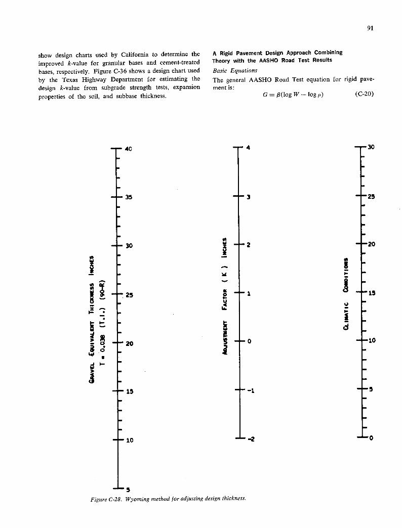
91

show design charts used by California to determine the A Rigid Pavement Design Approach Combining

improved k-value for granular bases and cement-treated Theory with the AASHO Road Test Results

bases, respectively. Figure C-36 shows a design chart used Basic Equations

by the Texas Highway Department for estimating the The general AASHO Road Test equation for rigid pave- design k-value from subgrade strength tests, expansion ment is: properties of the soil, and subbase thickness. G = (Iog W - log p) (C-20)

40 r3°

35 1-3

30 2 20

:

g _ 25 2 U 1 15

I— • I-.

20 0 10

LâJ - u

15 —1 5

10 .L._2

15

Figure C-28. Wyoming method for adjusting design thickness.

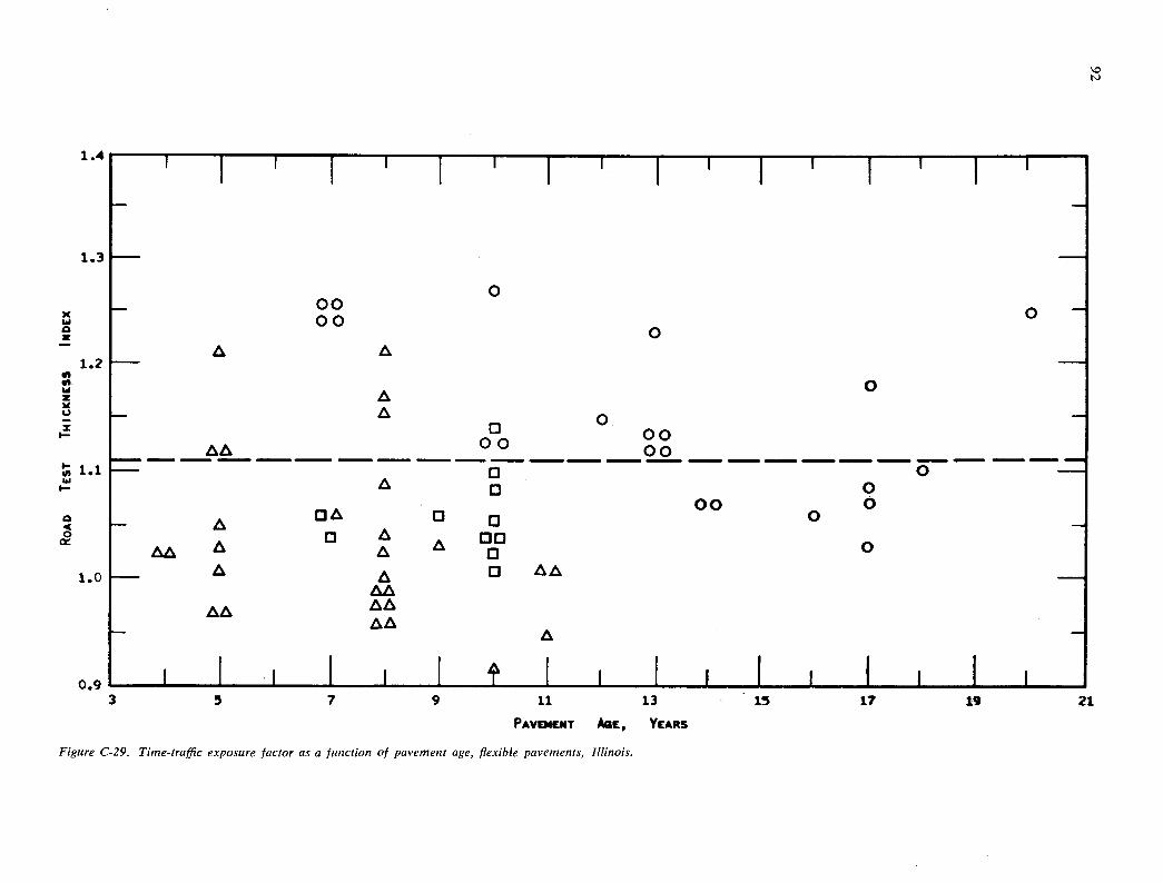
1.4

1.3

x w 0

1.2

z I I-

I- VI 1.1 I-

a 4 0

1.0

0.9

0 - 00 00

0 A A

0 A - A 0 00

AA 00 00 - 0 0 - A a 0

00 0 - A DA 13 0

AA A o A

A oo A 0 0 - A A 0 AA -

AA AA -

AA AA

I •I I I I I I I

3 5 7 9 11 13 15 17 19

21

PAVEJIENT AGE, YEARS

Figure C-29. Time-traffic exposure factor as a function of pavement age, flexibk pavements, Illinois.

t'J

2.0

1.8

1.6

1 -

0

-00

8R 0 0

0 -

- ___ ___ ___ ______AVERAa1. 8_ 0 0 -

- o 0 -

0 0 0 0 0

- 0 0 0 - 00 0 0

IIIIIIIIIIIIIIII

1.2

1.0

8

12 16 20 24 29

40

Pavurr A, Y*.s Figure C-30. Time-traffic exposure factor as a function of pavement age, rigid pavements, Illinois.

94

.20

Figure C-31. Regional map of Texas. Regions define areas of equivalent pavement behavior.

2 CBR 3 4 5 6 7 8 9 60 Is 20 25 30 40 50 50 0,

Gerivral Soil RatIng as Suborada 5uoose or base

Voru poor soograda S. Pair Pg good 5ub9radeJ Sub2 Good

USED. (CaSooronde's) Soil CiassifCOpiofl (3)

5O)n.m.

- High COiep,.SOSIbfllty

I I- a°

;. — — - SF

IML

- I

° L Civil AernrlgLt.s Adm. Soil - - - - - - Classification () - - -

I E-B Li

- FSoS SOC

- - - - C-S CBS 8*1

r,-4 con cc

L(o I

L_E-9 v-ID -

E lli 1 Bureau of Public Roads Soil Classificafior-i (5 ) - - -

I — itoorig Qi-Haaai A3 (ieoii5aa,a(_ — ipi,,iici AH (r.rHsOl.....

1A-a

a-s (A-s vOicanic materials mad have CBS of .00)

ILSearing Value lb. per sq. in. 161

(0 I I 20 I 3b I I 40 50 6Q_ 70

Modulus of Soil Reaction 'k inlb/sq. in/in. 171 — (00 50 I 200 I 250 I soo 1 -

California Boaring Ratio 'CaR' 1°) 11(11 i1111 5 3 4 S 6 7 8 9 10 5 20 25 30 40 50 60 70 00 00 0

All interrelationships are approximate. Actual tests are required to determine CBS, 4, etc.

For basic idea, see Porter, 0.J .,"Foundations for Flexible Pavements." Proc. ORB, Vol. 22 (1942) pp. 100-136.

.,. . (3) Relationships from .BgBqerimg Manual. Chap.XX, Office of the Chief of in WulCis Engineers • War Dept. (March 1943). See also Middlebrooke, TA.. and Bertram,

-. . G.E .0511 Tests for Design of Runway Pavements. Proc.URB, Vol. 22 (1942) G = a logarithmic function of the ratio of loss in 73.

values eatimated from old lAS clausiffeatiss systes. serviceability at any time to the total potential (3)0cc EnglneeriugMaeual. A-6 and A-7 soils cut off at COB 15 rather than

loss when Pt = 1.5; (6) See Middlebrooko and Bertram, p. 184. Bearing values at 0.1 in. deflection;

= a function of design and load variables that in (7) See, item (3) . k is factor used in Westergaard's Aasalyois for thickness of

fluences the shape of the p versus W serviceability curve: Figure C-32. Interrelationships of soil classifications, California

W = axle load applications at time p is observed; bearing ratios, bearing values, and k-values.

p = a function of design and load variables that de-notes the expected number of axle load applica-tions to a serviceability index of 1.5; and

500

400

z -'-5

300 0 w -J

200

100

0 0 JO ZO 30 40 50 60 70 80

R — VA LUE

Figure C-33. k-value vs R-value.

700

600 50 0

500

CQQ

300

270

0 C 0 I

200

150

100

700

600

500

400

300 z -S

U, a- i 200

1000 900 800 700

600 a. 500

Uj Cl, 400

95

-0 CL

00

0 50 a

50 0 0.1 0.2 0.3 0.4 0.5 0.6 0.7 0.8 0.9 - 1.0

25 0 0.1 0.2 0.3 0.4 0.5 0.6 0.7 0.0 U.V 1.0 Figure C-35. Effect of various thicknesses of cement-treated

THICKNESS OF CEMENT- TREATED BASE, FEET

THICKNESS OF SUBBASE - FEET bases on k-values.

Figure C-34. Effect of various thicknesses of granular subbases on k-values.

k VALUES

TEXAS TRIAXIAL STRENGTH CLASS - NATURAL MATERIAL

XCLASS 3.5 OR BETTER MATERIAL, UPPER 6' TO BE A NONPUMPING MATERIAL.

EXAMPLE: TO DETERMINE CORRECTED k VALUE WHERE NATURAL MATERIAL TRIAXIAL STRENGTH IS 5.3, P.V.R. = 3/4" AND 6" OF SUBBASE IS TO BE USED.

Figure C-36 k-values for all coin pactable natural haterials

96

p = present serviceability index, a number derived by formula for estimating the serviceability rating from measurements of certain physical features of a pavement.

For Road Test conditions,

3.63(L1 + L5 ) 55° /3=1.00+ (D+ 1)846 L,52 (C-21)

and

log p= 5.85 + 7.35 log (D + 1) -4.62 log (L1 +L0) +3.28 log L., (C-22)

in which

L1 = load on one single axle or on one tandem-axle set, kips;

L, = axle code (1 for single axle and 2 for tandem axle); and

D thickness of rigid pavement slab, inches.

Because the equations for both 3 and p contain the terms L1, L2, and D, the solution of the general equation becomes involved, particularly when solving for D, the factor normally sought in pavement design. Solution of the equation can be simplified, however, by expressing all load factors in terms of a common denominator. In the Guide the chosen denominator is the 1 8,000-lb single-axle load For use in the design equation the following factors are now fixed: L5 = 18 kips; and L2 = 1.

The equation for W (the number of equivalent 18-kip single-axle applications a given design will carry) becomes:

log W= log p+ (G/ 18) (C-23)

in which

1.00+ 3.63(18 + 1)5.20 /3=

(D + 1) 8.46 13.52

1.624 X 10 = 1.00 + (C-24) (D + 1) 8.46

and

log p= 5.85 + 7.35 log (D + 1) -4.62 log(18 + 1) + 3.28 (log 1)

= 7.35 log (D + 1) - 0.06 (C-25)

Therefore, Eq. C-23 becomes

log W=7.35 log (D+l)-_0.06 1l.624x107

+ (D+l)S.46

(C-26)

The Road Test equation then provides a basis for design involving these factors:

Axle load relationships (through equivalencies). Number of equivalent load applications to be carried

(through traffic factor). Slab thickness required.

These relationships were developed at the Road Test

with pavements having a great number of other design factors held constant. These fixed factors included:

Modulus of elasticity of concrete. Concrete strength. Modulus of subgrade reaction. Jointed, doweled pavements only. A particular set of environmental conditions. An actual life span of two years.

Modifications by Theory

It is considered desirable to incorporate into the design procedures as many of these factors as possible. Those factors that can be evaluated by theory or by experience can be used immediately. Other factors, such as slab continuity, may not be sufficiently well defined for inclu-sion at this time. However, if provisions are made for inclusion in the design equation of such additional factors, they can be held constant for the present, and used as further information becomes available. Two possible ap-proaches to combining the Road Test equation and theory are:

Use theoretical formulas as the basic design form, and modify the load term or the final answer for repetitions.

Use the Road Test equation as the basic form, and use theory to modify it for variations in physical constants.

The second approach appears to be the more valid, par-ticularly in view of the fact that, at the Road Test, failure was not defined as cracking (overstress) but as a reduction in serviceability which usually does not occur until some time after initial cracking.

To evaluate the effect of variations in physical factors on pavement life, Road Test performance data were ana-lyzed from a different approach. The first step was to make a comparison of the pavement strains actually mea-sured on the Road Test and the stresses calculated from several of the theoretical formulas available, including Westergaard, Spangler, and Pickett. Although the mea-sured stresses differ from the calculated values, both the Westergaard and Spangler equations do an excellent job of linearizing the Road Test measurements. The Spangler equation was selected for use because of its simplicity, and because it shows a good correlation with Road Test mea-surements. The Spangler equation is:

3.2 P / (r =

D2 I )

(C-27a)

or, in a more general form,

JPI' a\ (C-27b)

in which

= maximum concrete tensile stress, psi; P = wheel load, pounds; D = thickness of concrete slab, inches; a1 = the distance in inches from the corner of the slab

to the center of the area of load application. It is

97

taken equal to (aV2) where a is the radius of a circle equal in area to the loaded area;

J = a coefficient dependent on load transfer characteris- tics or slab continuity; westergaard's ratio of relative stiffness

= [ ZD3 ¼ _2)]

(C-28a) 12(1

E = Young's modulus of elasticity for the concrete, psi; k = modulus of subgrade reaction, psi/in.; and = Poisson's ratio for the concrete.

To simplify the work and without damage to the theory, Poisson's ratio (p.) was fixed at 0.20.

The fixed value of Poisson's ratio results in a simplified equation for the radius of relative stiffness.

1= (ZD/11.52)1/4 (C-28b)

Ten inches also represents approximately the average value for the range of loads of major interest at the Road Test, so a1 was fixed at 10.

No other modifications were made in the Spangler equa-tion, because the relationship between the physical con-stants is linearized. The coefficient J will need additional analysis for protected corner or continuously reinforced slabs before it can be used in design; however, it cancels out in the present equation.

Using Eq. C-27b, stresses were calculated for various combinations of Road Test variables. The ratio of the modulus of rupture to these calculated stresses (Se /cr) was compared with axle applications. For any given load and terminal serviceability level (Pt) the relationship between S0 /o and W is defined by

log W=a+blogF (C-29)

in which

W = number of applications of the given load to a given terminal serviceability;

F = S0/cr; modulus of rupture (concrete);

a- = stress calculated from Eq. C-27b; a = a constant; and b = the slope of the curve.

The fact that the slope of this line for a given p is nearly constant for the range of loads tested lends confidence to the use of this approach.

Using these slopes for 1 8-kip single-axle loads gives the following relationship between p and b for a range of p = 1.5 to 2.5.

b = 4.22 - 0.32 p (C-30)

Thus, Eq. C-29 becomes:

log W= a + (4.22— 0.32 p) logF (C-31)

Differentiating Eq. C-29 gives

log W=(b) log F (C=32)

Then the difference in life between a pavement with given

physical properties described by F (e.g., the the Road Test pavements) and one with modified physical properties (F')

could be expressed as

log W' - log W = b(log F' - log F) (C-33a)

Rearranging terms gives

log W' = log W + b (log F' — logF) (C-33b)

in which

W' = the number of load applications to reach service-ability p for a pavement with physical properties as described by F'; and

F' = the Sc /cr ratio for the properties other than at the Road Test.

Combining Eqs. C-30 and C-33b gives

log W' = log W + (4.22 - 0.32 p)(log F' - log F) (C-34)

Assumptions

At this point two important assumptions must be made:

The variation in life (W) for different loads at the same level of Se/a- is accounted for by the basic Road Test equation, and is covered in this design procedure by the traffic equivalence factors.

Any change in F due to varying the physical con-stants for concrete E, k, D, and S0 will have the same effect

on W as varying slab thickness D, and this relationship is

defined by Eq. C-29.

Combined Equations

With these assumptions it is possible to incorporate theory into the Road Test results. Combining Eqs. C-26 and C-34 gives

log W' = 7.35 log (D + 1) —0.06 + 1

1.624 X 10 + (D+l)8•46

+ (4,22 - 0.32 p) (log F' - log F) (C-35)

Expanding, using definitions given previously, gives

log F' - log F = log = log ( 2r)() = log(-)(-)

(C-36)

jpf a1\(D2\(_1 ;7= —i -k 1-- )i -

J(

I—a, ~ 1' —1) ~ r --a

- a\ (C-37) J'\ IJ\l'—a1 J

1' [[fz' D3\f11.52\1¼

Tl1.s27s.. ZD3 )]

= (Z'/Z)¼ (C-38)

98

/ z D3 \ 1/411.52)

10 1- a -

Z' D\

1_al_ ¼ () -10

[z¼D-K_lo(1.842)I[

1.842

- 1.842 Z'¼D~-1O(1.842)]

Z¼D%- 18.42 Z'¼DY4 18.42

.i /z'\¼ /Z¼DPY4- 18.42

Z'¼D~i- 18.42) (C-40)

F' 1 ,_ /S6'\IJ z'\¼ /4fZD%-18.42log=log)-))

Z'¼D%- 18.42

(C-4 1 a)

At this point it is convenient to evaluate the physical con-stants for the Road Test.

Evaluation of Physical Constants

Eq. C-26 was developed from pavements at the Road Test that had fixed physical constants as follows: E (28-day static) = 4.2 X 106 average. This value was selected be-cause at this age the percentage gain in strength is relatively low, regardless of cement type used.

k (gross, 30-in, plate) = 60 average. S6 (28-day, third-point loading, AASHO T 97-57) =

690 average. J = 3.2 (assumed value for illustration).

Substituting these values:

4.2 X 106 Z=E/k= 60 = 7 X lO

F'

R-6-900 S6 73.2\f_z' \716.27D%- 18.42 log=Iog _) 16 ¼ 27)

Z'1/4 D-Y, - 18.42

1.132\1 = log [2is3(

18.42) 1 (C-41b)

Z'¼ j Assembling the general equation:

log W' = 7.35 log(D + 1) - 0.06 + G

1.624 X 10

1 + (D+ 1)8.46

\1 + (4.22_0.32P)[lo 1.132

4

_J]

(2ls3J(_- 18.42 I

(C-42)

By further substitution of Road Test values, J' = 3.2 and E = 4.2 X 106, these terms are removed from considera-tion. Further, by removing the primes for ease of presen-tation and substituting working stress (/) (0.75 times modulus of rupture) for modulus of rupture (se), the equation becomes:

log W=7.35 log(D+ 1) -0 G

.06+ 1,624x 10

1+ (D + 1)8.46

+ (4.22 - 0.32 p)[log ()( 1/4)] (C-43)

When one is using this equation it is necessary to enter with the same basic factors as defined previously. That is, (1) 28-day static E, (2) k, gross with 30-in, plate, and (3) f, 0.75 times S.. If tests other than these are used, it will be necessary to adjust the value by correlation.

Other Factors

Subbase Quality.-As brought out in the Guide, the Road Test equation, and thus this equation, is based on pave-ments that had a sand-gravel subbase. It is possible to include a term, Q, in the design equation to permit varia-tion of this subbase quality. The term Q is arbitrary and can be based only on experience and the small amount of data available from Experiment Design 3 at the Road Test. Such a term would involve the question: "How will the design k be maintained for the life of the pavement?" The desirability of including this term points up the need for "satellite" research in this field in order to make a proper evaluation of subbases.

Regional Factor.-The Road Test equations do not pro-vide any clue to the variations in pavement life due to variation in environment or weather. This could become an important factor in areas different from the Road Test site. If desirable, a regional factor (R) can be included in the design equation to account for differences in frost penetration, rainfall, daily temperature variation, and other weather factors. This factor is not evaluated on the design chart, but it is believed that an effort should be made to establish the scale for such a factor.

Idealized Equation

To summarize the foregoing, all the factors mentioned could be included in a complete design equation of the form:

333(4.5 - Pt) log W=7.351og(D-F 1) -0.06+ log 0. 1.624X 10

I + (D + 1)8.46

_____ -1.l32\'l18.421

+ (4.22 - 0.32 Pt)[log 7)

(D:y4 D% -

+ C1Q - C, + C3R (C-44)

in which the factors involved are as defined previously.

Determination of k for Use with the Rigid Pavement Design Equations

The k-value (modulus of subgrade reaction) used on the AASHO design chart for rigid pavements is somewhat smaller than the k-value to which engineers are accus-tomed. That used in rigid pavement design is usually the so-called "elastic k." The k used as a basis for develop-ment of the Interim Guide for rigid pavements is the "gross

(C-39)

99

k." The gross k is smaller than the elastic k because the total deflection of the plate is considered in the calculations.

The elastic k was used in this development because its values are generally in the range with which engineers are familiar, and it comes closer to duplicating the original Westergaard assumptions. Therefore, when one is com-paring the results of the design charts with the AASHO design charts, this difference in the k-value should be taken into consideration. The studies at the AASHO Road Test showed the following correlation between the two k-values:

The expression for percentage is:

P8 = (A8'/A)(100) (C-47)

in which

P8 = required steel, percent; A8' = cross-sectional area of steel, square inches; and A = cross-sectional area of concrete, square inches.

Eq. C-46 can be changed to the total required steel area by multiplying by width:

in which

kE =l.77kG (C-45)

\A8'=(

FLW2, ) z (C-48a)

= elastic modulus of support, pci; and kG = gross modulus of support, pci.

The problem of determining a k-value for use in rigid pavement design is compounded by other factors, such as the ability of a material to maintain its initial value over the life of the pavement. As an indication of the range of k-values to be expected, one can look at the supporting materials used at the AASHO Road Test. The basic sub-grade material was an A-6 clay, Texas Triaxial Class 5.6. When used directly, this material had a gross k of 20 to 30. A subbase material was provided for most of the sections of the AASHO Road Test. This subbase material was a sandy gravel, Texas Triaxial Class 3.7. Six to 9 in. of this material resulted in a gross k-value of 50 to 75, with an average of 60, equivalent to an elastic k-value of about 108. The Interim Guide is based• primarily on the performance of these sections.

From this information it appears that, for use with the Guide, an elastic k of 100 to 200 pci might be expected from good granular subbases about 6 in. thick, and an elastic k of 200 to 400 might be expected from stabilized material about 6 in. thick.

Expressing Steel Requirements for Jointed Concrete

Pavement as a Percentage

The Interim Guide for design of rigid pavements uses the conventional subgrade drag theory for calculating the re-quired steel percentage of reinforced jointed concrete pave-ments. This formula is

A8= FL W

2f (C-46)

in which

A8 = cross-sectional area of steel, square inches per foot of slab width;

F = friction coefficient of subbase; L = slab length, feet;

= allowable working stress of steel, psi; and W = weight of slab per square foot.

The result is in units of square inches per foot of slab width. These units are not compatible with the generally accepted current practice of expressing the steel require-ments as a percentage. Therefore, an equation for con-version to percentage is derived as follows.

The W term is simply a combination of the pavement thickness and concrete density:

W=(D)(w) (C-49)

in which

D = pavement thickness, inches; and w = concrete unit weight, lb/cubic foot.

Combining Eqs. C-48a and C-49 gives

FLDwZ A8'=

2f (C-48b)

Rearranging terms gives

A8' _ FLw (C-48c)

-:-- 2/

The left-hand side of this equation is the ratio of steel area to concrete area; therefore:

- (FL w)(l00) (C-50a)

2t

To be dimensionally correct;

8= [FLw 1

2)14418j [100] (C-SOb)

Because the unit weight of concrete is generally taken as 145 to 150 pcf, Eq. C-SOb is approximately equal to:

FL Ps = 27; (C-50c)

OVERLAY DESIGN PROCEDURES

An overlay may be placed on an in-service pavement to improve its structural strength, its riding quality, and its skid resistance, or a combination of any of these. Only procedures pertaining to improving structural strength are considered here. The procedures used by Oklahoma, Cali-fornia, and the Corps of Engineers are discussed.

Oklahoma Method

Figure C-37 shows a flow chart summarizing the Okla-homa method of overlay design. The design method is based on providing a present serviceability index of 2.0 after 20 years of service, and consists of three separate submethods.

For the pavement condition submethod, data obtained

100

PAVEMENT CoNDITION

RATING

CONDI T_ON PREDICTED

sv _______________ & DEPRECIATION DEFLECTION

PAVEMENT

cTEO LIFE

I 10 YEARS

AGE

OVERLAY THICKNESS DEFLECTION AVERAGE _______

ADJUST FOR AMOUNT OF ALL ANSWERS DEFLECTION

I

________

j

LOOKED AT FOR (STAINED BY: By SECTION SEASONS OVERLAY I FINAL THICKNESS

FLEXIBLE PAVE!ENT j

REQUIRED AMOUNT OFl

EXISTIN

PAVEMENT PAVEMENT DESIGN PROCEDLE STRESS STRESS OVERLAY I

Figure C-37. Oklahoma overlay design procedure for flexible pavements. Developed from information from Hartronft (88).

from a detailed pavement condition survey are used to assign a pavement rating from 0 to 100 percent (failed to excellent). The rating and the pavement age, counting from the last major rehabilitation or new construction, is used with Figure C-38 to obtain the expected design life and the percentage of deterioration expected at an age of 10 years. This information is then used with Figure C-39 to estimate the Benkelman beam deflection. The required overlay thickness is then determined by means of Figure C-40.

The second submethod (Fig. C-37) consists of measur-ing the deflection under a 9,000-lb wheel load. The de-flections are averaged for areas of similar deflection, and the average is adjusted for seasonal variation. The cor-rected deflection value is used to determine the required overlay thickness of asphaltic concrete from the nomo-graph in Figure C-40. The amount of overlay is a func-tion of the average deflection greater than 0.022 in. This limiting value was derived from a field study of in-service pavements that found the maximum allowable pavement deflection, under a 9,000-lb wheel load, should not exceed 0.037 in. for a pavement to perform satisfactorily for 20 years. A safety factor of 33 percent and a fatigue factor of 33 percent were used to convert to a 15,000-lb design wheel load, which is equivalent to a maximum deflection value of 0.022 in.

The third submethod (Fig. C-37) is a reevaluation of the design using the Oklahoma Department of Highways' flexible pavement design method. The existing pavement structure is subtracted from the pavement structure derived by reevaluation to arrive at the overlay thickness required.

California Method

The California method is based on measurement of deflec-tion under a 7,500-lb wheel load. The deflection profile for a section is separated into categories of fill, cut, cracked, uncracked, etc., and an 80 percentile deflection value is obtained. The 80 percentile is used to avoid placing too much emphasis on isolated conditions by using the maxi-mum value or underdesigning through use of the average. A limiting value of deflection, based on the existing pave-ment structure thickness and the number of equivalent

wheel loads expected during the design life, is selected from Figure C-4 1. This value is subtracted from the 80 percentile deflection and expressed as a percent reduc-tion. The percent reduction is then used with Figure C-42 to determiiie the amount of overlay thickness required. No attempt is made with this method to quantitatively measure the condition of the existing pavement.

Corps of Engineers Methods

The Corps of Engineers has developed design procedures for rigid and flexible overlays over both pavement types. The procedures are presented in the Corps of Engineers' manuals EM 1110-45-303 (54) and TM 5-824-2 (55). They may be used for any pavement, but were developed primarily for runways and taxiways at airports. The U.S. Air Force has adopted basically the same procedures.

The following sections describe the Corps of Engineers' procedures for rigid overlay over rigid pavements and flexible overlay over rigid pavements. The flexible over flexible and the rigid over flexible are not discussed because these procedures are essentially the same as the regular design procedure for each pavement type.

Rigid Overlays Over Rigid Pavements

The procedure of rigid overlays over rigid pavements is based on one of two equations, depending on whether a partial bonded or an unbonded overlay is used. The un-bonded overlay is considered for conditions where an asphaltic concrete layer is placed between the old and the new layers of portland cement concrete pavement.

The design equations for each condition are as follows:

Partial bonded:

h0 - 1.4Vh14 - Ch1 (C-51)

Unbonded:

h0 = Vh 2 - Ch2 (C-52)

in which

h0 = thickness of rigid overlay slab, inches; he = thickness of new pavement from regular rigid pave-

ment design analysis, inches;

100

90

SO

'V

40

101

u•ri•riiu•rim UUIIiW1UNA• lUI1UIWA•UV4Ul

uurn•iirn•uvu•i

miwraui•uu•u UU1UH1iWA•lN••l

rwrnv•rii••••• iiviragr••uuu•• uriiu•••uuuu --U...... 24 28

Hartionft (88, p. 68).

60

1 0 ;50

30

20

10

0 0 4 8 12 16 20

Mc ( YCARS

Figure C-38. Life curves for flexible pavements. Source

h = thickness of the existing pavement, inches; and C = a coefficient depending on the condition of the

existing slab, ranging from 0.35 for badly cracked slabs to 1.0 for slabs in excellent condition.

Eq. C-52 is for the noncontinuous case, because Eq. C-Si assumes the slabs not to work independently. In the equation, C is not a true estimate of the load-carrying capacity, but rather a factor qualitatively associated with previous performance as measured by the amount of crack-ing present. The choice of the proper C for existing pave-ment may often be only a rough estimate, as no quantita-tive guidance is given, other than general ranges.

Flexible Overlays Over Rigid Pavements

The procedure of flexible overlays over rigid pavements is based on an empirical formula that assigns a structural equivalency to relate the thickness of asphaltic concrete and portland cement concrete, as follows:

1= 2.5(Fh - h) (C-53)

DCPRCCIATION (% AT 10 YEARS Ac)

20 30 40 50 60 70 80 90 100

I I 0 5 10 15

I IIII I IlIII III IlIIIII

20 25 30 35

II

40

1 11111 1

45 50

BoxcI..MAN Bus DCrI.CCTION (INcHES x io, 9000 La. Wucci. LOAD)

Figure C-39. 9,000-lb wheel load deflection vs depreciation for Interstate pavements (flexible).

A. C. OVCR&.A'V REQuIaw FOR 15,000 Lu. W. L. SuPPORt

10 12 13 14

ill

60'

1 11111 11111111 11111111 111111111

20 30 40 50 70 so 90 100

BENKELNAN Bus Dcn..cCyIoN (Iacsis x 10, 9000 Lu. WHEEL LOAD)

Figure C-40. Asphaltic concrete overlay requirement based on Benkelman bean? deflections.

100

80 I.1 x

60 - so

40

30

20

(1 w -j S..

10

8,

102

TRAVTIC INDEX (1954 DEsIGN PROCEDURE)

--

__ -

V.1 1.0 10.0 100.0

1000.0

EQUIVALENT 5000 La. WHEEL LOADS (E.W.L.) MILLIONS

Figure C-41. Variation in tolerable deflection based on asphaltic concrete fatigue tests.

in which

= thickness of the overlay; F = a factor related to condition of the existing pave-

ment;

hd = the exact design thickness determined from the regular rigid pavement design procedures; and

h = the existing pavement thickness, inches.

A critical step in this design procedure is the selection

0

P. oln 0 0 0 a

NOI.&33iJQ N "OI,L3nMH 101333d

4 200

103

of the proper F-value, which is a function of the subgrade modulus of support and the type of loading expected. The F-value decreases as the support value increases.

COMPUTER PROGRAMS

Programs for solving flexible and rigid pavement design equations for SN and D are shown in Figures C-43 and C-44.

PROGRAM IAN (INPUT, OUTPUT, TAPE5-INPUT) PROGRAM IAN (INPUT, OUTPUT, TAPE5-INPUT)

000003 REAL K 000003 REAL K

000003 1 FORMAT (3F12.4) 000003 1 FORMAT (3F12,4)

000003 2 FORMAT (*NOT YET*15, 4F18.4) 000003 2 FORMAT (*NOT YET*15,4F18.4)

000003 3 FORMAT (*_GOT ONE*15, 4F18.4) 000003 3 FORMAT(*-GO1' ONE*15,4F18.4)

000003 6 FORMAT(*1 INPUT VALUES*3F18.4///) 000003 6 FORMAT (*1 INPUT VALUES3F18.4///)

000003 5 READ 1, G,W,SN 000003 5 READ 1, G,W,DA 000015 PRINT 6, G,W,SN 000015 PRINT 6, G,W,DA 000027 N=0 000027 N=0 000030 IF (EOF,5) 90,10 000030 IF (EOF,5)90,10

000033 10 N-N-i-i 000033 10 N-N+1 000035 K-G / (.4+1094./(SN+1) **5.19) 000035 K_G/(i.+16240000./(DA+1.)**8.46)

000045 SC=1.0501*10.**(.1068*K)*W**.1068_1. 000045 DC_1.0190*10.**(.1360*K)*W**.1360_1.

000060 IF((ABS(SC-SN)-.01LE.0.0) GO TO 30 000060 IF((ABS(DC-DA)-.05).LE.0.0) GO TO 30

000065 PRINT 2,N,G,W,SN,SC 000065 PRINT 2,N,O,W,DA,DC

000102 IF (N.5.25) GO TO 5 000102 XF(N.EQ.25) GO TO 5 000104 SN-SC 000104 DA-DC

000106 GO TO 10 000106 GO TO 10

000106 30 PRINT 3,N,G,W,SN,SC 000106 30 PRINT 3, N,G,W,DA,DC

000 124 GO TO 5 000124 GO TO 5

000125 90 STOP 000125 90 STOP

000127 END 000127 END

Figure C-43. Program for solving flexible pavement equation Figure C-44. Program for solving rigid pavement equation.

APPENDIX D

PROCEDURE FOR THE RESILIENT MODULUS TEST

TEST METHOD FOR DYNAMIC TRIAXIAL LOADING OF

SOIL OR AGGREGATE SPECIMENS UNDER

CONTROLLED STRESS

Scope

This method describes a procedure for testing, under dynamic loading with controlled stress conditions, un-treated aggregate specimens or aggregate specimens bound with flexible binders. Stress control is defined as the process of applying a predetermined axial load to a speci-men and measuring the axial deformation or strain that the specimen undergoes. Data obtained with this pro-cedure can be used in determining damping characteristics and moduli of resilience of the test specimen. The equip-ment for dynamic triaxial loading under controlled stress consists of three basic components:

Triaxial cell with loading piston and transducers for measuring load and strain or deflection.

Controlled cyclic air supply. Power amplifier with oscillograph.

Apparatus

1. Loading piston. Triaxial cell of suitable size for testing 21/2 -in. X 5-in.

and 6-in. X 12-in, specimens. Cyclic air supply. Daytronics LVDT Model No. DS1500-B45804, suit-

ably mounted for measuring the deformation due to the applied load.

Timer to regulate speed of testing machine at fre-quencies up to 3 cps.

Load cell, for controlling stress. Daytronics 300 CP amplifier. Daytronics type 60 plug-in module. Honeywell Model No. 906C Visicorder.

Rubber membranes of suitable size for confining 21/2 -in. X 5-in, and 6-in. X 12-in, test specimens.

0-rings, of suitable size to fasten membrane to base and top caps.

Procedure

1. Measure and record height and weight of specimen. Place suitable membrane around specimen. Note:

For testing under unconfined conditions (confining pres-sure = 0) omit items 2, 3, 6, and 7.

Secure membrane to top cap and base cap with 0-rings.

Place specimen with membrane in triaxial cell. Extend rod from main load piston to top cap of

specimen. Apply predesignated confining pressure. Make appropriate rod correction. Set air pressure at inlet to give predesignated load

stress to the specimen.

104

9. Record applied load and deflection on an oscillograph trace at the following designated intervals:

INTERVAL NUMBER OF CYCLES

1 0-10 2 50-60 3 500-510 4 1,000-1,010 5 2,000-2,0 10 6 5,000-5,010 7 10,000-10,010 8 20,000-20,010

If the specimen fails during test, report the number of cycles to failure.

Calculations

1. From the data reported here, develop the following plots:

Hysteresis loops at representative cycles for each interval. Permanent set as a function of number of load repetitions.

2. For each test interval, make the following calcula-tions:

Damping coefficient—Damping coefficient, n, is equal to the energy absorbed during a dynamic cycle, D, divided by the total energy applied during the cycle, W. Modulus of resilience—Modulus of resilience, MB, is equal to the dynamically applied deviator stress (so-) divided by the resulting dynamic elas-tic (recoverable) strain (€) and is given by

M11 = ( T)/€ (o — cr)/E (D-l)

APPENDIX E

ALTERNATE SIGNIFICANCE STUDY

A significance study was also conducted with traffic as the dependent variable because the original Road Test equa-tions are presented in that form. To make structural number (SN) a dependent variable, trial and error solu-tions are required. Such solutions are simplified by the use of nomographs as found in the AASHO Interim Guide design procedures. The results of the significance study with traffic as the dependent variable can be used to esti-mate errors in pavement life (load applications) due to errors in each of the design variables.

In the following sections, the general concepts of each analysis method are discussed; these concepts are then applied to each of the equations and the resulting findings are presented. In the concluding section, the implications of these findings are discussed in terms of their meaning to the pavement design engineer.

ANALYSIS MODELS

The differentiation technique consists of differentiating each of the equations in terms of each considered variable. This technique can be used to give only an indication of the independence of the variables in the error analysis. For example, in the flexible pavement equation it can answer such a question as: Is an error in traffic due to an error in the structural number also dependent on the mag-nitude of the soil support or is the relation independent of soil support? Due to a fundamental limiting assumption

of differentiation, the derived expressions are applicable only over small changes in the variables. For example, error in traffic cannot be considered for errors of 5 per-cent in the regional factor, because this magnitude violates the small-interval principle of differentiation.

For the computer analysis, the error in traffic is investi-gated for three levels of magnitude for every independent variable, and for three levels of error magnitude. The magnitudes of the variables considered are given in fac-torial form in Tables E-1 and E-2 for flexible and rigid pavements, respectively. One level of magnitude for each variable is the property of the material at the AASHO Road Test as indicated in the Guides. The three levels of error considered in the analysis are ± 1, 5, and 10 percent of the possible or normal range of each variable, with the exception of the concrete flexural strength and modulus of elasticity. These two factors generally have a greater range under field conditions, so a value of 20 percent was used as a maximum in lieu of 10 percent.

RESULTS OF DIFFERENTIATION ANALYSIS

Flexible Pavements

The flexible pavement equation derived in Appendix C was used as the basis for this study because it contains all the parameters considered in the Guides.

(100.372(8-3)) (SN + 1 )9.36( lOG/fl) W 1 = (E-1)

1.535 R

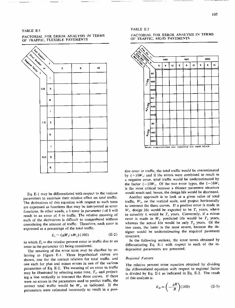
TABLE E-1

FACTORIAL FOR ERROR ANALYSIS IN TERMS OF TRAFFIC, FLEXIBLE PAVEMENTS

TABLE E2

FACTORIAL FOR ERROR ANALYSIS IN TERMS OF TRAFFIC, RIGID PAVEMENTS

105

3 6 10

0.5 3

6

1.0 3

6

5.0 3

6

Eq. E-1 may be differentiated with respect to the various parameters to ascertain their relative effect on total traffic. The derivatives of this equation with respect to each term are expressed as functions that may be interpreted as error functions. In other words, a 8 error in parameter i of 8 will result in an error of 8 in traffic. The relative meaning of each of the derivatives is difficult to comprehend without considering the amount of traffic. Therefore, each error is expressed as a percentage of the total traffic.

E= (W/W)(1OO) (E-2)

in which Ei = the relative percent error in traffic due to an error in the parameter (i) being considered.

The meaning of the error term may be clarified by re-ferring to Figure E-1. Three hypothetical curves are shown, one for the correct relation for total traffic, and one each for plus and minus errors in one of the various parameters of Eq. E-2. The meaning of an error in traffic may be illustrated by selecting some time, T, and project-ing a line vertically to intersect the three curves. If there were no errors in the parameters used to predict traffic, the correct total traffic would be W, as indicated. If the parameters were estimated incorrectly to result in a posi-

MEN minuuiuuiiu u:iuiuuaaai :iuiuuuuuu :u•ui•uuaa MEN

NINE MEN u:iiuuiuuuu Seven computations are required for each block.

tive error in traffic, the total traffic would be overestimated by (+)8W,; and if the errors were combined to result in a negative error, total traffic would be underestimated by the factor (—)8W. Of the two error types, the (—)8W is the most critical because a thinner pavement structure would result and, hence, the design life would be shortened.

Another approach is to look at a given value of total traffic, W, on the vertical scale, and project horizontally to intersect the three curves. If a positive error is made in W, design life would be expected to be T1 years, where in actuality it would be T years. Conversely, if a minus error is made in W, predicted life would be T 2 years, whereas the actual life would be only Ta years. Of the two cases, the latter is the most severe, because the de-signer would be underestimating the required pavement structure.

In the following sections, the error terms obtained by differentiating Eq. E-1 with respect to each of the in-dependent parameters are presented.

Regional Factors

The relative percent error equation obtained by dividing the differentiated equation with respect to regional factor is divided by Eq. E-1 as indicated in Eq. E-2. The result of this analysis is:

E1 = (_)(1oo) (E-3)

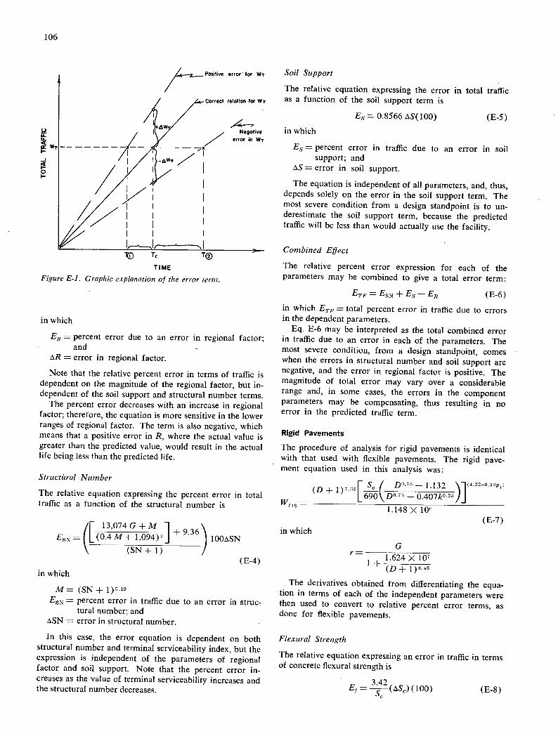
106

Positive error for Wi

Correct relotion for Wi

14-1 Negotive

error in Wi I TIME

Figure E-1. Graphic explanation of the error term.

in which

ER = percent error due to an error in regional factor; and- -

AR = error in regional factor.

Note that the relative percent error in terms of traffic is dependent on the magnitude of the regional factor, but in-dependent of the soil support and structural number terms.

The percent error decreases with an increase in regional factor; therefore, the equation is more sensitive in the lower ranges of regional factor. The term is also negative, which means that a positive error in R, where the actual value is greater than the predicted value, would result in the actual life being less than the predicted life.

Structural Number

The relative equation expressing the percent error in total traffic as a function of the structural number is

Soil Support

The relative equation expressing the error in total traffic as a function of the soil support term is

Es = 0.8566 ES( 100) (E-5)

in which

E2 = percent error in traffic due to an error in soil support; and

= error in soil support.

The equation is independent of all parameters, and, thus, depends solely on the error in the soil support term. The most severe condition from a design standpoint is to un-derestimate the soil support term, because the predicted traffic will be less than would actually use the facility.

Combined Effect

The relative percent error expression for each of the parameters may be combined to give a total error term:

ETF = EsN + E - ER (E-6)

in which ETF = total percent error in traffic due to errors in the dependent parameters.

Eq. E-6 may be interpreted as the total combined error in traffic due to an error in each of the parameters. The most severe condition, from a - design standpoint, comes when the errors in structural number and soil support are negative, and the error in regional factor is positive. The magnitude of total error may vary over a considerable range and, in some cases, the errors in the component parameters may be compensating, thus resulting in no error in the predicted traffic term.

Rigid Pavements

The procedure of analysis for rigid pavements is identical with that used with flexible pavements. The rigid pave-ment equation used in this analysis was:

(D + 1)7.:5[_ s. _(_D°•75 - 1.132 \1(422_032pt [690\,D0.T5 _0.407k0.25 )]

1.148 x 10' "Vt's

r 13,074G+M 1 Es=([(0.4M+ 1,094)j + 9.36)

(SN + 1) (E-4)

in which

in which

G r =

+ 1.624 X 10' 1 (D + 1)8.46

(E-7)

M= (SN+1)' ESN = percent error in traffic due to an error in struc-

tural number; and SN = error in structural number.

In this case, the error equation is dependent on both structural number and terminal serviceability index, but the expression is independent of the parameters of regional factor and soil support. Note that the percent error in-creases as the value of terminal serviceability increases and the structural number decreases.

The derivatives obtained from differentiating the equa-tion in terms of each of the independent parameters were then used to convert to relative percent error terms, as done for flexible pavements.

Flexural Strength

The relative equation expressing an error in traffic in terms of concrete flexural strength is

Ei= 3.42

(5)(loo) (E-8)

107

in which

E1 = percent error in traffic due to an error in flexural strength; and

- error in flexural stieiigtli.

The error is dependent on the magnitude of flexural strength, but independent of all other factors. The error decreases as the flexural strength increases. The most severe condition occurs at the lower values of flexural strength, and for underestimates of flexural strength.

Sub grade Modulus Term

The relative equation expressing an error in total traffic in terms of subgrade reaction is

0.348

E1 - k°75[D°75 - 18.42(k/E)°25] 100k (E-9)

in which

Ek = percent error in traffic due to an error in sub-grade modulus; and

Ak = error in subgrade modulus.

In this case, the magnitude of error is dependent on the pavement thickness, the modulus of elasticity, and the subgrade modulus, and is independent of the flexural strength and of serviceability terms. As the magnitude of the three dependent parameters increases, the percent error decreases. Therefore, the most severe conditions are for the lower values of pavement thickness, concrete modulus, and subgrade modulus, and for underestimation of the subgrade modulus.

Pavement Thickness

The relative equation expressing the error in total traffic in terms of an error in pavement thickness is

(D + l)7.11; 2.42 X 10 7.35— 2.3(D + l)( (D + 1)11.46 + 1.624 )]

D° 75 - 1.132 3.42 (D + 1)[ D°

75 - 0.407k°25 ]

X 100D (E-10)

Here the equation is dependent on pavement thickness and subgrade modulus, but independent of the other terms. Generally, the error decreases as the pavement thickness increases and as the subgrade modulus decreases. Thus, the most severe conditions are for low values of pavement thickness, for high values of subgrade modulus, and when the pavement thickness is underestimated.

Modulus of Elasticity

The relative equation expressing the error in total traffic in terms of an error in the modulus of elasticity is

15.75 k°25 (E'•25)

I l00E EE=_[[D0751842(k/E)095]

(E-11)

Here the equation is negative and the error is dependent on subgrade modulus, pavement thickness, and modulus of elasticity. The relative percent error decreases as pave-ment thickness and modulus of elasticity increases, and as the subgrade modulus decreases. Therefore, the most se-vere conditions occur with small values of pavement thick-ness and modulus of elasticity, with high values of sub-grade modulus, and when the modulus of elasticity is overestimated.

Combined Effect

As was the case for flexible pavements, the error terms may be combined to obtain an expression for the total error, as follows:

ETJI = E1 + EK + ED - EE (E-12)

in which ET11 = total percent error in traffic due to errors in the dependent parameters.

The most severe condition for an error in the rigid pave-ment equation is when the flexural strength, subgrade modulus, and pavement thickness are underestimated, and the modulus of elasticity is overestimated. As was the case for flexible pavements, the errors may be compensating or compounding.

RESULTS OF NUMERICAL ANALYSIS

Using a computer, Eqs. E-1 and E-7, for flexible and rigid pavements, respectively, were solved for the combination of values given in Tables E-1 and E-2. These data were then plotted on graphs to quantitatively express error in traffic due to the error in each of the parameters. The percent error in traffic was computed for each solution using Eq. E-2, and the results are plotted on the ordinate of each graph. The percent error in variables is listed on the abscissa.

As would be expected, the numerical solutions mani-fested the same dependence or independence of variables on the percent error terms as was found with the differ-entiation method. The primary variance from the dif-ferentiation solution is that the sign of the 8 term has an influence on the magnitude of the relative percent error terms for the computer solution, whereas this was not the case for the differentiation equations.

Flexible Pavements

The following sections give the numerical solutions of the equations for errors in regional factor, structural number, and soil support.

Regional Factor

Figure E-2 shows the effect of errors in regional factor on the total traffic. The numerical data indicate that a plus or a minus error in regional factor has the same effect on error in traffic. The quantitative data indicate that for a regional factor equal to 0.5 and a 10 percent possible error, the error in total traffic may be 100 percent. For a more commonly used regional factor value of 1.0, the

ED = I

C

0

Ui

ae

/ /

/ /

/ /

/ /

/ /

/ /

/

/ 7'!

100

40

108

I I I

140 - -

Soil Support 3,6,10 R.gionol Facto, 5.010,0.5

120 - -

100 - R 0.5

60- -

% Error in Regional Facto,

Figure E-2. Error in traffic for error in regional factor.

0

% Error in SN

Figure E-3. Error in traffic for error in structural number.

I SN 1,3,6 S 3,6,10

/ /

/ /

/ /

/ /

/ /

/ /

/

-

% Error In Soil Support

Figure E-4. Error in traffic for error in soil support.

design life might be up to 50 percent in error if a value of 0.5 or 1.5 were used instead; i.e., a 10 percent error in regional factor.

Structural Number

Figure E-3 shows the effect of an error in the structural number on the total traffic. The error differs with the sign of the structural number error, with minus values resulting in the greatest percent errors. The error in structural number directly reflects errors in layer equivalence coeffi-cients used to estimate the structural number. For exam-ple, if a layer equivalence of 0.44 is used for 6 in. of asphaltic concrete, but the layer coefficient is actually 0.35, the structural number would be overestimated by 0.54.

Soil Support

Figure E-4 shows the effect of an error in soil support on the total traffic. In this case the magnitude of the error function depends on sign, with the negative values resulting in the greatest percent error.

Combined Effects

109

Of the three parameters considered, an error in structural number has by far the most significant effect on the life. Next in order is soil support and then regional factor, although the two have approximately equal influence.

Figure E-5 shows the maximum combined error in total traffic in terms of the parameter errors. The maximum error is for an overestimate of SN and S, and for under-estimates of R, for values of SN = 1.0 and R = 0.5. Note that the relative percent error in the overestimate of total traffic varies from 40 percent for a 1 percent error in each of the parameters, to 245 percent for 10 percent error in the parameters. Also shown on the graph is a curve for maximum errors for the AASHO Road Test conditions. For these (S = 3.0 and R = 1.0), the error ranges from 25 percent for a 1 percent error in parameters to 175 percent for a 10 percent error. The curves for an under-estimate of total traffic are also shown. The same com-binations of parameters produce the maximum under-estimate curves, but the signs are negative.

An example problem, at this point, serves to illustrate the meaning of Figure E-5. Following is an example prob-lem where parameter values were incorrectly assumed and the resulting error was presented:

VALUE PARAMETER TRAFFIC

FACTOR ASSUMED CORRECT ERROR(%) ERROR(%)

R 0.75 1.0 +5.0 —25 SN 3.0 2.75 —5.0 —82 S 4.0 3.5 —5.0 —53

Total —160

The values in the last column were obtained from Fig-ures E-2, E-3, and E-4, and summed algebraically to give a resulting underestimate of 160 percent in traffic. The parameter values selected are similar to the AASHO Road Test values; hence, by entering Figure E-5 with a 5 per-cent error a total underestimating error of 160 percent is obtained, which is the same as above. The problem dem-onstrates the use of the figures, but any combination of error values may be used with Figures E-2, E-3, and E-4, and summed as per the example problem. The 5 percent error in structural number is intended to reflect a 9 per-cent error in the asphaltic concrete layer coefficient. In this example, 6 in. of asphaltic concrete were assumed, and a value of 0.44 was used in lieu of the correct value of 0.40. The resulting error in traffic reveals the importance of assuming the proper value of structural layer coefficient in design.

Rigid Pavements

The numerical solutions of Eq. E-2 for errors in thickness and in flexural strength for rigid pavements are shown in Figures E-6 and E-7, respectively. An error in the modulus of elasticity or in subgrade reaction shows no significant effect on the total traffic for the values of the parameter investigated.

ET°ESN+Es — ER

100—

— % Error in Independent Parameter,

%Error .

Figure E-5. Maxi,num combined error in Wt for errors in parameters using flexible pavements equation.

Pavement Thickness

The relative percent error in total traffic varies as to whether an overestimate (+) or an underestimate (-) of the pavement thickness is made, with an overestimate re-sulting in the greatest percent error. The rigid pavement thickness term is not subject to the possible error of the structural number term in the flexible equation, because pavement thickness is used directly and no conversion is made. The possibility of error in pavement thickness comes during construction where a section may be built thicker or thinner than the planned dimensions due to problems in grade control or other associated construction problems. Figure E-6 indicates that a small variation of thickness will have a tremendous influence on pavement life. This offers one possible explanation to the isolated failures often observed.

Flexural Strength

The relative percent error in total traffic also varies as to whether an overestimate or underestimate is made of the flexural strength. As shown in Figure E-7, overestimating results in the greatest percent error. Also, the graph shows that the smaller the magnitude of the flexural strength, the larger the relative percent error in total traffic. It should

110

% Error In Pvmt. Thickness 0

Figure E-6. Percent error in traffic for error in pavement thickness D.

also be pointed out that of all the parameters considered in the rigid pavement equation, flexural strength has the greatest probability of variation under field conditions.

Combined Effect

An error in the pavement thickness term has the most sig-nificant effect on an error in pavement life as reflected by the total traffic term. Figure E-8 shows the maximum per-cent error in traffic obtained by summarizing the compo-nent errors for pavement thickness and flexural strength. The maximum error for overestimation occurs with an overestimation of pavement thickness and flexural strength for values of D = 5 and flexural strength = 400 psi. Also included is the maximum curve for the AASHO Road Test conditions of D = 8 in. and flexural strength = 690 psi. For this curve, the relative percent error in traffic ranges from 10 percent to 150 percent for 1 and 10 percent errors in the parameters, respectively. Also presented are the errors in underestimation for the same conditions.

% Error in Flee Strength S.

Figure E-7. Percent error in traffic for error in flexible strength.

An example problem follows to illustrate the significance of these graphs. Because the subgrade modulus term and the modulus of elasticity term do not influence the error, the following problem was developed using D and S:

VALUE PARAMETER W,

FACTOR ASSUMED CORRECT ERROR (%) FACTOR (%)

D 8 7.5 —6.2 —42 S0 690 650 —6.7 —19

Total —61

In this problem, values of pavement thickness of 8 in. and a flexural strength of 690 psi were assumed in design, but, due to factors such as poor construction control, the actual values in the field were 7.5 and 650 psi. This results in an underestimate of design life, as shown in the last column. When the two factors are combined, it is seen that the pavement life may be 61 percent less than intended. (Be-cause equal percentages were not used, Figure E-8 cannot be used to obtain the combined answer.)

100

Figure E-8. Combined percent error in flexural strength and pavement thickness.

111

Published reports of the

NATIONAL COOPERATIVE HIGHWAY RESEARCH PROGRAM

are available from:

Highway Research Board National Academy of Sciences

2101 Constitution Avenue Washington, D.C. 20418

Rep. No. Title

—* A Critical Review of Literature Treating Methods of Identifying Aggregates Subject to Destructive Volume Change When Frozen in Concrete and a Proposed Program of Research—Intermediate Report (Proj. 4-3(2)), 81p., $1.80

1 Evaluation of Methods of Replacement of Deterio- rated Concrete in Structures (Proj. 6-8), 56 p., $2.80

2 An Introduction to Guidelines for Satellite Studies of Pavement Performance (Proj. 1-1), 19 p., $1.80

2A Guidelines for Satellite Studies of Pavement Per- formance, 85 p.+9 figs., 26 tables, 4 app., $3.00

3 Improved Criteria for Traffic Signals at Individual Intersections—Interim Report (Proj. 3-5), 36 p., $1.60

4 Non-Chemical Methods of Snow and Ice Control on Highway Structures (Proj. 6-2), 74 p., $3.20

5 Effects of Different Methods of Stockpiling Aggre-gates—Interim Report (Proj. 10-3), 48 p., $2.00

6 Means of Locating and Communicating with Dis-abled Vehicles—Interim Report (Proj. 3-4), 56 p. $3.20

7 Comparison of Different Methods of Measuring Pavement Condition—Interim Report (Proj. 1-2), 29 p., $1.80

8 Synthetic Aggregates for Highway Construction (Proj. 4-4), 13p., $1.00

9 Traffic Surveillance and Means of Communicating with Drivers—Interim Report (Proj. 3-2), 28 p., $1.60

10 Theoretical Analysis of Structural Behavior of Road Test Flexible Pavements (Proj. 1-4), 31 p., $2.80

11 Effect of Control Devices on Traffic Operations— Interim Report (Proj. 3-6), 107 p., $5.80

12 identification of Aggregates Causing Poor Concrete Performance When Frozen—Interim Report (Proj. 4-3(1)), 47p., $3.00

13 Running Cost of Motor Vehicles as Affected by High- way Design—Interim Report (Proj. 2-5), 43 p., $2.80

14 Density and Moisture Content Measurements by Nuclear Methods—Interim Report (Proj. 10-5), 32 p., $3.00

15 Identification of Concrete Aggregates Exhibiting Frost Susceptibility—Interim Report (Proj. 4-3(2)), 66 p., $4.00

16 Protective Coatings to Prevent Deterioration of Con- crete by Deicing Chemicals (Proj. 6-3), 21 p., $1.60

17 Development of Guidelines for Practical and Realis- tic Construction Specifications (Proj. 10-1), 109 p., $6.00

18 Community Consequences of Highway Improvement (Proj. 2-2), 37 p., $2.80

19 Economical and Effective Deicing Agents for Use on Highway Structures (Proj. 6-1), 19 p., $1.20

* Highway Research Board Special Report 80.

Rep. No. Title

20 Economic Study of Roadway Lighting (Proj. 5-4), 77 p., $3.20

21 Detecting Variations in Load-Carrying Capacity of Flexible Pavements (Proj. 1-5), 30 p., $1.40

22 Factors Influencing Flexible Pavement Performance (Proj. 1-3(2)), 69 p., $2.60

23 Methods for Reducing Corrosion of Reinforcing Steel (Proj. 6-4), 22 p., $1.40

24 Urban Travel Patterns for Airports, Shopping Cen- ters, and Industrial Plants (Proj. 7-1), 116 p., $5.20

25 Potential Uses of Sonic and Ultrasonic Devices in Highway Construction (Proj. 10-7), 48 p., $2.00

26 Development of Uniform Procedures for Establishing Construction Equipment Rental Rates (Proj. 13-1), 33 p., $1.60

27 Physical Factors Influencing Resistance of Concrete to Deicing Agents (Proj. 6-5), 41 p., $2.00

28 Surveillance Methods and Ways and Means of Com- municating with Drivers (Proj. 3-2), 66 p., $2.60

29 Digital-Computer-Controlled Traffic Signal System for a Small City (Proj. 3-2), 82 p., $4.00

30 Extension of AASHO Road Test Performance Con- cepts (Proj. 1-4(2)), 33 p., $1.60

31 A Review of Transportation Aspects of Land-Use Control (Proj. 8-5), 41 p., $2.00

32 Improved Criteria for Traffic Signals at Individual Intersections (Proj. 3-5), 134 p., $5.00

33 Values of Time Savings of Commercial Vehicles (Proj. 2-4), 74 p., $3.60

34 Evaluation of Construction Control Procedures— Interim Report (Proj. 10-2), 117 p., $5.00

35 Prediction of Flexible Pavement Deflections from Laboratory Repeated-Load Tests (Proj. 1-3(3)), 117p., $5.00

36 Highway Guardrails—A Review of Current Practice (Proj. 15-1), 33 p., $1.60

37 Tentative Skid-Resistance Requirements for Main Rural Highways (Proj. 1-7), 80 p., $3.60

38 Evaluation of Pavement Joint and Crack Sealing Ma- terials and Practices (Proj. 9-3), 40 p., $2.00

39 Factors Involved in the Design of Asphaltic Pave- ment Surfaces (Proj. 1-8), 112 p., $5.00

40 Means of Locating Disabled or Stopped Vehicles (Proj. 34(1)), 40 p., $2.00

41 Effect of Control Devices on Traffic Operations (Proj. 3-6), 83 p., $3.60

42 Interstate Highway Maintenance Requirements and Unit Maintenance Expenditure Index (Proj. 14-I), 144 p., $5.60

43 Density and Moisture Content Measurements by Nuclear Methods (Proj. 10-5), 38 p., $2.00

44 Traffic Attraction of Rural Outdoor Recreational Areas (Proj. 7-2), 28 p., $1.40

45 Development of Improved Pavement Marking Ma- terials—Laboratory Phase (Proj. 5-5), 24 p., $1.40

46 Effects of Different Methods of Stockpiling and Handling Aggregates (Proj. 10-3), 102 p., $4.60

47 Accident Rates as Related to Design Elements of Rural Highways (Proj. 2-3), 173 p., $6.40

48 Factors and Trends in Trip Lengths (Proj. 7-4), 70 p., $3.20

49 National Survey of Transportation Attitudes and Behavior—Phase I Summary Report (Proj. 20-4), 71 p., $3.20

Rep. No. Title 50 Factors Influencing Safety at Highway-Rail Grade

Crossings (Proj. 3-8), 113 p., $5.20 51 Sensing and Communication Between Vehicles (Proj.

3-3), 105 p., $5.00 52 Measurement of Pavement Thickness by Rapid and

Nondestructive Methods (Proj. 10-6), 82 p., $3.80

53 Multiple Use of Lands Within Highway Rights-of- Way (Proj. 7-6), 68 p., $3.20

54 Location, Selection, and Maintenance of Highway Guardrails and Median Barriers (Proj. 15-1(2)), 63 p., $2.60

55 Research Needs in Highway Transportation (Proj. 20-2), 66 p., $2.80

56 Scenic Easements—Legal, Administrative, and Valua- tion Problems and Procedures (Proj. 11-3), 174 p., $6.40

57 Factors Influencing Modal Trip Assignment (Proj. 8-2), 78 p., $3.20

58 Comparative Analysis of Traffic Assignment Tech-niques with Actual Highway Use (Proj. 7-5), 85 p., $3.60

59 Standard Measurements for Satellite Road Test Pro- gram (Proj. 1-6), 78 p., $3.20

60 Effects of Illumination on Operating Characteristics of Freeways (Proj. 5-2) 148 p., $6.00

61 Evaluation of Studded Tires—Performance Data and Pavement Wear Measurement (Proj. 1-9), 66 p., $3.00

62 Urban Travel Patterns for Hospitals, Universities, Office Buildings, and Capitols (Proj. 7-1), 144 p., $5.60

63 Economics of Design Standards for Low-Volume Rural Roads (Proj. 2-6), 93 p., $4.00

64 Motorists' Needs and Services on Interstate Highways (Proj. 7-7), 88 p., $3.60

65 One-Cycle Slow-Freeze Test for Evaluating Aggre-gate Performance in Frozen Concrete (Proj. 4-3(1)), 21p., $1.40 .

66 Identification of Frost-Susceptible Particles in Con- crete Aggregates (Proj. 4-3(2)), 62 p., $2.80

67 Relation of Asphalt Rhcological Properties to Pave- ment Durability (Proj. 9-1), 45 p., $2.20

68 Application of Vehicle Operating Characteristics to Geometric Design and Traffic Operations (Proj. 3- 10), 38 p., $2.00

69 Evaluation of Construction Control Procedures—Aggregate Gradation Variations and Effects (Proj. 10-2A), 58 p., $2.80

70 Social and Economic Factors Affecting Intercity Travel (Proj. 8-1), 68 p., $3.00

71 Analytical Study of Weighing Methods for Highway Vehicles in Motion (Proj. 7-3), 63 p., $2.80

72 Theory and Practice in Inverse Condemnation for Five Representative States (Proj. 11-2), 44 p., $2.20

73 Improved Criteria for Traffic Signal Systems on Urban Arterials (Proj. 3-5/1), 55 p., $2.80

74 Protective Coatings for Highway Structural Steel (Proj. 4-6), 64 p., $2.80

74A Protective Coatings for Highway Structural Steel-.-- Literature Survey (Proj. 4-6), 275 p., $8.00

74B Protective Coatings for Highway Structural Steel— Current Highway Practices (Proj. 4-6), 102 p., $4.00

75 Effect of Highway Landscape Development on Nearby Property (Proj. 2-9), 82 p., $3.60

Rep. No. Title 76 Detecting Seasonal Changes in Load-Carrying Ca-

pabilities of Flexible Pavements (Proj. 1-5(2)), 37 p., $2.00

77 Development of Design Criteria for Safer Luminaire Supports (Proj. 15-6), 82 p., $3.80

78 Highway Noise—Measurement, Simulation, and Mixed Reactions (Proj. 3-7), 78 p., $3.20

79 Development of Improved Methods for Reduction of Traffic Accidents (Proj. 17-1), 163 p., $6.40

80 Oversize-Overweight Permit Operation on State High- ways (Proj. 2-10), 120 p., $5.20

81 Moving Behavior and Residential Choice—A Na- tional Survey (Proj. 8-6), 129 p., $5.60

82 National Survey of Transportation Attitudes and Behavior—Phase II Analysis Report (Proj. 20-4), 89 p., $4.00

83 Distribution of Wheel Loads on Highway Bridges (Proj. 12-2), 56 p., $2.80

84 Analysis and Projection of Research on Traffic Surveillance, Communication, and Control (Proj. 3-9), 48 p., $2.40

85 Development of Formed-in-Place Wet Reflective Markers (Proj. 5-5), 28 p., $1.80

86 Tentative Service Requirements for Bridge Rail Sys- tems (Proj. 12-8), 62 p., $3.20

87 Rules of Discovery and Disclosure in Highway Con- demnation Proceedings (Proj. 11-1(5)), 28 p., $2.00

88 Recognition of Benefits to Remainder Property in Highway Valuation Cases (Proj. 11-1(2)), 24 p., $2.00

89 Factors, Trends, and Guidelines Related to Trip Length (Proj. 7-4), 59 p., $3.20

90 Protection of Steel in Prestressed Concrete Bridges (Proj. 12-5), 86 p., $4.00

91 Effects of Deicing Salts on Water Quality and Biota —Literature Review and Recommended Research (Proj. 16-1), 70 p., $3.20

92 Valuation and Condemnation of Special Purpose Properties (Proj. 11-1(6)), 47 p., $2.60

93 Guidelines for Medial and Marginal Access Control on Major Roadways (Proj. 3-13), 147 p., $6.20

94 Valuation and Condemnation Problems Involving Trade Fixtures (Proj. 11-1(9)), 22 p., $1.80

95 Highway Fog (Proj. 5-6), 48 p., $2.40 96 Strategies for the Evaluation of Alternative Trans-

portation Plans (Proj. 8-4), 111 p., $5.40 97 Analysis of Structural Behavior of AASHO Road

Test Rigid Pavements (Proj. 1-4(1)A), 35 p., $2.60

98 Tests for Evaluating Degradation of Base Course Aggregates (Proj. 4-2), 98 p. $5.00

99 Visual Requirements in Night Driving (Proj. 5-3), 38 p., $2.60

100 Research Needs Relating to Performance of Aggre- gates in Highway Construction (Proj. 4-8), 68 p., $3.40

101 Effect of Stress on Freeze-Thaw Durability of Con- crete Bridge Decks (Proj. 6-9), 70 p., $3.60

102 Effect of Weldments on the Fatigue Strength of Steel Beams (Proj. 12-7), 114 p., $5.40

103 Rapid Test Methods for Field Control of Highway Construction (Proj. 10-4), 89 p., $5.00

104 Rules of Compensability and Valuation Evidence for Highway Land Acquisition (Proj. 11-1), 77 p., $4.40

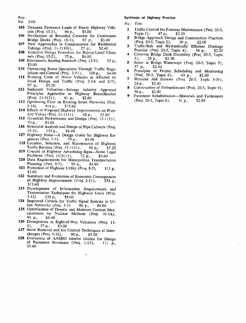
Rep. No. Title

Dynamic Pavement Loads of Heavy Highway Vehi- cles (Proj. 15-5), 94 p., $5.00 Revibration of Retarded Concrete for Continuous Bridge Decks (Proj. 18-1), 67 p., $3.40 New Approaches to Compensation for Residential Takings (Proj. 11-1(10)), 27 p., $2.40 Tentative Design Procedure for Riprap-Lined Chan- nels (Proj. 15-2), 75 p., $4.00 Elastomeric Bearing Research (Proj. 12-9), 53 p., $3.00 Optimizing Street Operations Through Traffic Regu- lations and Control (Proj. 3-11), lOOp., $4.40 Running Costs of Motor Vehicles as Affected by Road Design and Traffic (Proj. 2-5A and 2-7), 97 p., $5.20 Junkyard Valuation—Salvage Industry Appraisal Principles Applicable to Highway Beautification (Proj. 11-3(2)), 41 p., $2.60 Optimizing Flow on Existing Street Networks (Proj. 3-14), 414 p., $15.60 Effects of Proposed Highway Improvements on Prop- erty Values (Proj. 11-1(1)), 42 p., $2.60 Guardrail Performance and Design (Proj. 15-1(2)), 70 p., $3.60 Structural Analysis and Design of Pipe Culverts (Proj. 15-3), 155 p., $6.40 Highway Noise—A Design Guide for Highway En- gineers (Proj. 3-7), 79 p., $4.60 Location, Selection, and Maintenance of Highway Traffic Barriers (Proj. 15-1(2)), 96 p., $5.20 Control of Highway Advertising Signs—Some Legal Problems (Proj. 11-3(1)), 72 p., $3.60 Data Requirements for Metropolitan Transportation Planning (Proj. 8-7), 90 p., $4.80 Protection of Highway Utility (Proj. 8-5), 115 p., $5.60 Summary and Evaluation of Economic Consequences of Highway Improvements (Proj. 2-11), 324 p., $13.60 Development of Information Requirements and Transmission Techniques for Highway Users (Proj. 3-12) 239 p., $9.60 Improved Criteria for Traffic Signal Systems in Ur- ban Networks (Proj. 3-5) 86 p., $4.80 Optimization of Density and Moisture Content Mea-surements by Nuclear Methods (Proj. 10-5A), 86 p., $4.40 Divergencies in Right-of-Way Valuation (Proj. 11- 4), 57 p., $3.00 Snow Removal and Ice Control Techniques at Inter- changes (Proj. 6-10), 90 p., $5.20 Evaluation of AASHO Interim Guides for Design of Pavement Structures (Proj. 1-11), 111 p., $5.60

Synthesis of Highway Practice

No. Title

1 Traffic Control for Freeway Maintenance (Proj. 20-5, Topic 1), 47 p., $2.20

2 Bridge Approach Design and Construction Practices (Proj. 20-5, Topic 2), 30 p., $2.00

3 Traffic-Safe and Hydraulically Efficient Drainage Practice (Proj. 20-5, Topic 4), 38 p., $2.20

4 Concrete Bridge Deck Durability (Proj. 20-5, Topic 3), 28 p., $2.20

5 Scour at Bridge Waterways (Proj. 20-5, Topic 5), 37 p., $2.40

6 Principles of Project Scheduling and Monitoring (Proj. 20-5, Topic 6), 43 p., $2.40

7 Motorist Aid Systems (Proj. 20-5, Topic 3-01), 28 p., $2.40

8 Construction of Embankments (Proj. 20-5, Topic 9), 38 p., $2.40

9 Pavement Rehabilitation—Materials and Techniques (Proj. 20-5, Topic 8), 41 p., $2.80

105

106

107

108

109

110

111

112

113

114

115

116

117

118

119

120

121

122

123

124

125

126

127

128

T H E NATIONAL ACADEMY OF S C I EN C ES is a private, honorary organiza-

tion of more than 700 scientists and engineers elected on the basis of outstanding contributions to knowledge. Established by a Congressional Act of Incorporation signed by President Abraham Lincoln on March 3, 1863, and supported by private and public funds, the Academy works to further science and its use for the general welfare by bringing together the most qualified individuals to deal with scientific and technological problems of broad significance.

Under the terms of its Congressional charter, the Academy is also called upon to act as an official—yet independent—adviser to the Federal Government in any matter of science and technology. This provision accounts for the close ties that have always existed between the Academy and the Government, although the Academy is not a governmental agency and its activities are not limited to those on behalf of the Government.

THE NATIONAL ACADEMY OF ENGINEERING was established on December

5, 1964. On that date the Council of the National Academy of Sciences, under the authority of its Act of Incorporation, adopted Articles of Organization bringing the National Academy of Engineering into being, independent and autonomous in its organization and the election of its members, and closely coordinated with the National Academy of Sciences in its advisory activities. The two Academies join in the furtherance of science and engineering and share the responsibility of advising the Federal Government, upon request, on any subject of science or technology.

THE NATIONAL RESEARCH COUNCIL was organized as an agency of the National Academy of Sciences in 1916, at the request of President Wilson, to enable the broad community of U. S. scientists and engineers to associate their efforts with the limited membership of the Academy in service to science. and the nation. Its members, who receive their appointments from the President of the National Academy of Sciences, are drawn from academic, industrial and government organizations throughout the country. The National Research Council serves both Academies in the discharge of their responsibilities..

Supported by private and public contributions, grants, and contracts, and volun-tary contributions of time and effort by several thousand of the nation's leading scientists and engineers, the Academies and their Research Council thus work to serve the national interest, to foster the sound development of science and engineering, and to promote their effective application for the benefit of society.

THE DIVISION OF ENGINEERING is one of the eight major Divisions into which the National Research Council is organized for the conduct of its work. Its membership includes representatives of the nation's leading technical societies as well as a number of members-at-large. Its Chairman is appointed by the Council of the Academy of Sciences upon nomination by the Council of the Academy of Engineering.

THE HIGHWAY RESEARCH BOARD, organized November 11, 1920, as an agency of the Division of Engineering, is a cooperative organization of the high-way technologists of America operating under the auspices of the National Research Council and with the support of the several highway departments, the Federal Highway Administration, and many other organizations interested in the development of trans-

portation. The purpose of the Board is to advance knowledge concerning the nature and performance of transportation systems, through the stimulation of research and dissemination of information derived therefrom.

HIGHWAY RESEARCH BOARD NATIONAL ACADEMY OF SCIENCES—NATIONAL RESEARCH COUNCIL 2101 Constitution Av.nu. Washington, D. C. 20418

ADDRESS CORRECTION REQUESTED

NON-PROFIT ORG.

U.S. POSTAGE

PAID

WASHINGTON, D.C. PERMIT NO. 42970