1

Multidisciplinary Aircraft Conceptual Design

Optimisation Using a Hierarchical Asynchronous

Parallel Evolutionary Algorithm (HAPEA)

Presented at the Sixth ADAPTIVE COMPUTING IN DESIGN AND MANUFACTURE(ACDM 2004)APRIL 20th - 22nd, 2004 at ENGINEERS HOUSE, CLIFTON, BRISTOL, UK

University of Sydney

L. F. Gonzalez

E. J. Whitney

K. Srinivas

K.C Wong

Pole Scientifique - Dassault Aviation-

J. Périaux

2

Overview

PART 1 Multi-Objective Problems

PART 2

Test Cases and Applications .

Research in Evolution Algorithms for Aeronautical Design Problems (EAs)

PART 3

3

Multi-Criteria Problems

Aeronautical design problems normally require a simultaneous optimisation of conflicting objectives and associated number of constraints. They occur when two or more objectives that cannot be combined rationally. For example:

Drag at two different values of lift.

Drag and thickness.

Pitching moment and maximum lift.

4

…..Multi--Criteria Optimisation

Nixi

f ,...1)(

A multi-criteria optimisation problem can be formulated as: Minimise:

Subject to constraints:

Different Approaches: Traditional aggregating functions, and Pareto and Nash.

2 solution thedominates

1 solution thecase thisIn*

)2

()1

(

: if2

a vector thanlesspartially said is 1

a vector problem, onminimisatia For

xx

xi

fxi

fi

xx

Mkxk

hMjxj

g ,....10)(,....10)(

5

Pareto Optimality

Formally, the Pareto optimal set can be defined as the set of solutions that are non-dominated with respect to all other points in the search space, or that they dominate every other solution in the search space except fellow members of the Pareto optimal set. For two solutions x and y (in minimisation form):

, dominates : : 1...

, nondominated w.r.t. : : 1...

, dominates x : : 1...

i i i

i i i

i i i

rel x y x y if f x f y M

rel x y x y if f x l f y M

rel x y y if f x f y M

For a problem in M objectives, this is called the 'relationship' operator. In practice we compute an approximation to the continuous set, by assembling .or each player, as can be seen in Figure 2, whereby information is exchanged

.

1 2 3, , .....* * * *ParetoSet x x x x

6

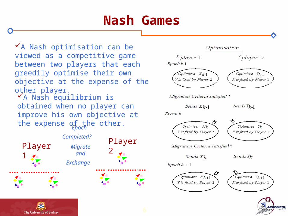
Nash Games

A Nash optimisation can be viewed as a competitive game between two players that each greedily optimise their own objective at the expense of the other player.

A Nash equilibrium is obtained when no player can improve his own objective at the expense of the other.

Player 1

Player 2

Epoch

Completed? Migrate

and

Exchange

7

The Problem…

Problems in aeronautical design optimisation: Traditional optimisation methods will fail to find the real answer in

most real engineering applications. Fitness functions of interest are generally multimodal with a

number of local minima. Sometimes the optimum shape/s is not obvious to the designer. The fitness function will involve some numerical noise.

Most aerodynamic design problems will need to be stated in multi-objective form.

Modern aeronautical design uses CFD (Computational Fluid Dynamics) and FEA almost exclusively.

CFD has matured enough to use for preliminary design and optimisation.

The internal workings of validated in-house solvers are essentially inaccessible from a modification point of view (they are black-boxes).

8

… The Solution…. Why Evolution?

Techniques such as Evolution Algorithms can explore large variations in designs. They also handle errors and deceptive sub-optimal solutions with aplomb.

They are extremely easy to parallelise, significantly reducing computation time.

They can provide optimal solutions for single and multi-objective problems.

EAs successively map multiple populations of points, allowing solution diversity.

They are capable of finding a number of solutions in a Pareto set or calculating a robust Nash game.

9

What Are Evolution Algorithms?

Crossover Mutation

Fittest

Evolution

Computers perform this evolution process as a mathematical simplification.

EAs move populations of solutions, rather than ‘cut-and-try’ one to another.

EAs applied to sciences, arts and engineering. Aerofoil and wing design, crew scheduling, control loops,etc.

Based on the Darwinian theory of evolution Populations of individuals evolve and reproduce by means of mutation and crossover operators and compete in a set environment for survival of the fittest.

10

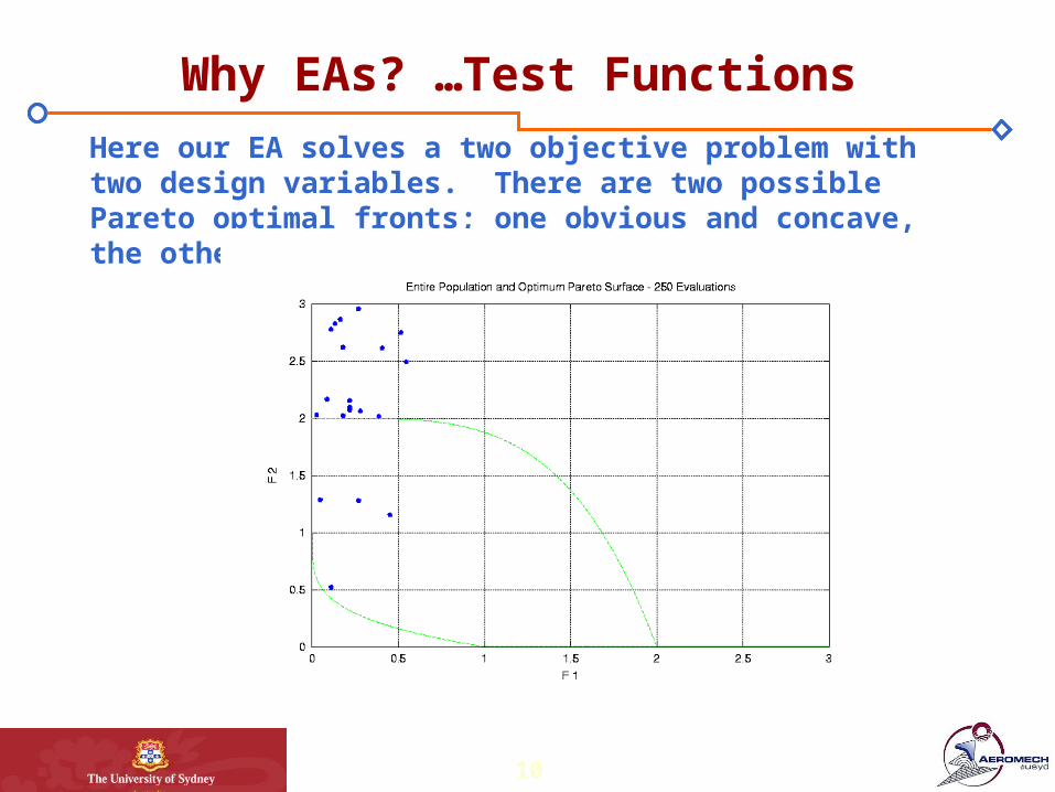
Why EAs? …Test Functions

Here our EA solves a two objective problem with two design variables. There are two possible Pareto optimal fronts; one obvious and concave, the other deceptive and convex.

11

“The Central Difficulty”

Evolutionary techniques are … still … very … slow!

(Often involving hundreds or thousands of separate flow computations)

Therefore, we need to think about ways of speeding up the process…

12

Hierarchical Topology-Multiple Models

Model 1precise model

Model 2intermediate

model

Model 3approximate

model

Exploration

Exploitation We use a technique that finds optimum solutions by using many different models, that greatly accelerates the optimisation process.

Interactions of the layers: solutions go up and down the layers.

Time-consuming solvers only for the most promising solutions.

Asynchronous Parallel Computing

Evolution Algorithm Evaluator

Hierarchical Topology

Parallel Computing and Asynchronous Evaluation

Synchronous Evaluationdifferent speed

EvolutionStrategy

Synchromous Evaluator

1 population (n individuals)

1 population (n individuals)

Single population

Hierarchical populations

ES Sync

ES ES

ES ES ES ES

Sync

Sync

Sync Sync Sync Sync

Each population has to go through a fixed number of generations before migration can take place

Since migration is global, the different populations will have to wait for the slowest one before exchanging individuals

The whole population is passed to the evaluator.

All the individuals of a given generation need to be evaluated before proceeding to the next generation

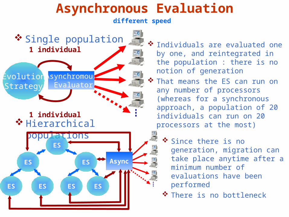
Asynchronous Evaluationdifferent speed

EvolutionStrategy

Asynchromous Evaluator

1 individual

1 individual

Single population

Hierarchical populations

ES

ES ES

ES ES ES ES

Async

Since there is no generation, migration can take place anytime after a minimum number of evaluations have been performed

There is no bottleneck

Individuals are evaluated one by one, and reintegrated in the population : there is no notion of generation

That means the ES can run on any number of processors (whereas for a synchronous approach, a population of 20 individuals can run on 20 processors at the most)

15

Asynchronous Evaluation…

Fitness functions are computed asynchronously. Only one candidate solution is generated at a time, and only

one individual is incorporated at a time rather than an entire population at every generation as is traditional EAs.

Solutions can be generated and returned out of order.

No need for synchronicity no possible wait-time bottleneck. No need for the different processors to be of similar speed. Processors can be added or deleted dynamically during the

execution. There is no practical upper limit on the number of processors

we can use. All desktop computers in an organisation are fair game.

16

….Asynchronous Evaluation…

Offspring are not sent as a complete 'block' to the parallel machines. A candidate is generated at a time, and sent to any idle processor where it is

evaluated at its own speed. After evaluation return to optimiser and check if accepted for insertion into

the main population or rejected. New selector operator because offspring cannot now be compared one against

the other, or even against the main population due to the variable-time evaluation.

Recently evaluated offspring are compared to a previously established rolling-benchmark and if successful, we replace (according to some rule) a pre-existing individual in the population.

A separate evaluation buffer, which provides a statistical 'background check' on the comparative fitness of the solution.  Buffer size 2 x PopSize

We compare it with the selection buffer by assembling at random a small subset called the tournament Q = [q1,q2,q3,…qn] and check that the individual is not dominated by any member of Q.

Q =1/2B (Strong selective pressure), Q =1/6B (weak selection pressure). Compare to past individuals (both accepted and rejected) -inserted or not   If accepted us strategy for replacement replace-worst-always method in this

paper.

Generate candidate

Send to idle processor

If evaluation completed send back

to optimiser

Compare to a tournament and if successful replace

Assign fitness

Compare to accepted and rejected

individuals –insert into the population

17

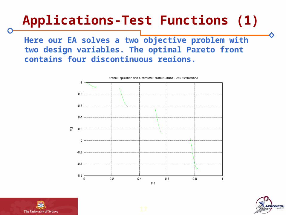
Applications-Test Functions (1)

Here our EA solves a two objective problem with two design variables. The optimal Pareto front contains four discontinuous regions.

18

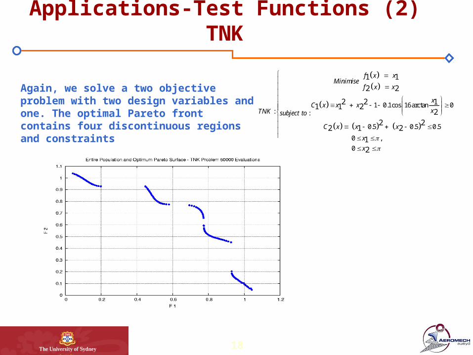
Applications-Test Functions (2) TNK

1 0.1cos 16arctan 0: :

0.5 0.5 0.5

0 ,

0

1 1

2 2

2 2 11 1 2

22 2

2 1 2

12

f x xMinimise

f x x

xC x x x

xTNK subject to

C x x x

x

x

Again, we solve a two objective problem with two design variables and one. The optimal Pareto front contains four discontinuous regions and constraints

19

Asynchronous Test: One Dimensional Nozzle

X-Distance

Ma

chN

um

be

r

0 0.5 10.4

0.6

0.8

1

1.2Target Mach Number

Generated Mach No.

Target Nozzle Shape

Generated Nozzlw Shape

Y-Nozzle half width

20

Synchronous, Single Population, Viscous model

Pop size = 207 processors

45mn

21

Asynchronous, Multiple Models, Viscous only

12mn

Pop size = 107 processors

22

CPU Times for HAPEA

Method CPU Time No of evaluations

Single Pop, Viscous, Traditional EA

45m 27s 12m 8s

2127 1137

Hierarchical Asynchronous

12m 6s 3m 58s

726 112

23

Real –world applications

Constrained aerofoil design for transonic transport aircraft 3% Drag reduction

UAV aerofoil design

-Drag minimisation for high-speed transit and loiter conditions.

-Drag minimisation for high-speed transit and takeoff conditions.

Exhaust nozzle design for minimum losses.

24

Real –world applications … (2)

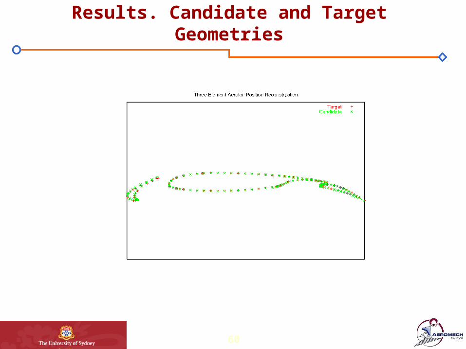
Three element aerofoil reconstruction from surface pressure data.

UCAV MDO Whole aircraft multidisciplinary design.Gross weight minimisation and cruise efficiency Maximisation. Coupling with NASA code FLOPS 2 % improvement in Takeoff GW and Cruise Efficiency

AF/A-18 Flutter model validation.

25

Case Studies

Multidisciplinary Aircraft Conceptual DesignCase Studies.

26

UCAV Conceptual Design.

Problem Definition: Find conceptual design parameters for a UCAV, to minimise two objectives:

Gross weight min(WG) Cruise efficiency min(1/[MCRUISE.L/DCRUISE])

We have six unknowns:

Lower Bound

Upper Bound

Aspect Ratio 3.1 5.3

Wing Area (sq ft) 600 1400

Wing Thickness 0.02 0.09

Wing Taper Ratio

0.15 0.55

Wing Sweep (deg)

22.0 47.0

Engine Thrust (lbf)

30500 50000

27

Mission Definition

Cruise 40000 ft, Mach 0.9, 400 nm

Landing

Release Payload 1800 Lbs

Maneuvers at Mach 0.9

Accelerate Mach 1.5, 500 nm

20000 ft

Engine Start and warm up

Taxi

Takeoff

Climb

Descend

Release Payload 1500 Lbs

Description Requirement

Range [R, Nm] 1000

Cruise Mach Number [Mcruise]

1.6

Cruise Altitude [hcruise, ft] 40000

Ultimate Load Factor [nult] 12

Takeoff Field Length [sto, ft] 7000

28

Solver

The FLOPS (FLight OPtimisation System) solver developed by L. A. (Arnie) McCullers, NASA Langley Research Center was used for evaluating the aircraft configurations.

FLOPS is a workstation based code with capabilities for conceptual and preliminary design of advanced concepts.

FLOPS is multidisciplinary in nature and contains several analysis modules including: weights, aerodynamics, engine cycle analysis, propulsion, mission performance, takeoff and landing, noise footprint, cost analysis, and program control.

FLOPS has capabilities for optimisation but in this case was used only for analysis.

Drag is computed using Empirical Drag Estimation Technique (EDET) - Different hierarchical models are being adapted for drag build up using higher fidelity models.

29

Two Approaches

Solved via :

Nash theory

and

Pareto Optimality.

30

Implementation

Nash Approach.

-Two hierarchical trees, with two levels, population size of 40.

Player 1

Player 2

Epoch

Completed? Migrate

and

Exchange

- Information exchanged (epoch) after 50 function evaluations. Variables split:-Player One: Aspect ratio, wing thickness and wing sweep; Maximises cruise efficiency.

-Player Two:Player Two: Wing area, engine thrust and wing taper; Minimises gross weight.

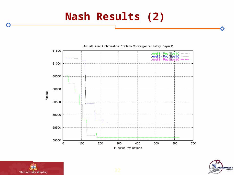
- Run for 600 function evaluations, but converged after 300.

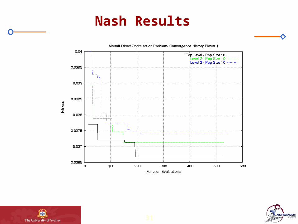
31

Nash Results

32

Nash Results (2)

33

Nash Results (3)

Variables Nash Equilibrium

Aspect Ratio 5.13

Wing Area (sq ft) 618

Wing Thickness 0.021

Wing Taper Ratio 0.17

Wing Sweep (deg) 28

Engine Thrust (lbf) 33356

Gross Weight (Lbs) 62463

Cruise Efficiency MCRUISE.L/DCRUISE

23.9

34

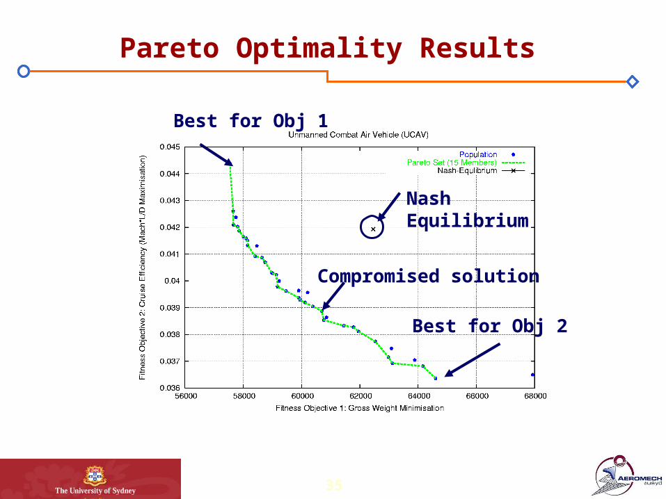
Implementation

Pareto Optimality Approach - Single Population.

- Population size of 40.

- Parallel computations, run asynchronously.

- Run for 600 function evaluations.

Asynchromous Evaluator

1 individual

1 individual

Single population

35

Pareto Optimality Results

Best for Obj 1

Best for Obj 2

Compromised solution

Nash Equilibrium

36

Comparison Results

Variables Pareto Member

0

Pareto Member 3

Pareto Member 7

Nash Equilibrium

Aspect Ratio 4.76 5.23 5.27 5.13

Wing Area (sq ft) 629.7 743.8 919 618

Wing Thickness (t/c)

0.046 0.050 0.041 0.021

Wing Taper Ratio 0.15 0.16 0.17 0.17

Wing Sweep (deg) 28 25 27 28

Engine Thrust (lbf) 32065 32219 32259 33356

Gross Weight (Lbs)

57540 59179 64606 62463

Increasing Cruise Efficiency

Decreasing Gross Weight

MCRUISE.L/DCRUISE22.5 25.1 27.5 23.9

Nash Point

37

Comparison Results (2)

Nash Equilibrium

Upper Bound

Lower Bound

Nash Design

38

Subsonic Transport Design and OptimisationProblem Definition: Find conceptual design parameters for a subsonic medium size

transport aircraft .

Gross weight min(WG)

The aircraft has two wing-mounted engines, and the number of passengers and crew is fixed to 200 and 8 respectively.

The aircraft is designed to cruise at 40000 ft and Mach 0.8.

We have six unknowns:Lower Bound Upper Bound

Aspect Ratio 7.0 13.1

Wing Area (sq ft) 1927 2872

Wing Thickness 0.091 0.235

Wing Taper Ratio 0.15 0.55

Wing Sweep (deg) 22.0 47.0

Engine Thrust (lbf)

32000 37000

39

Constraints and Implementation

Implementation The solution to this problem has been implemented

using a single population and parallel asynchronous evaluation, with the optimiser only considering a single objective.

After an empirical study, it was found that a small population size of 10 and buffer size of 30 produced acceptable results.

Constraints Constraints in this case are minimum takeoff

distance, moment coefficient for stability and control and range required. Violation of these constraints is treated with an rejection criteria.

40

Results

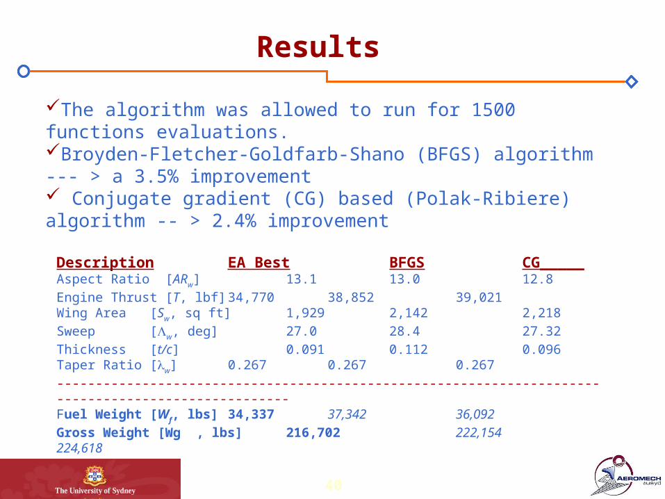
The algorithm was allowed to run for 1500 functions evaluations. Broyden-Fletcher-Goldfarb-Shano (BFGS) algorithm --- > a 3.5% improvement Conjugate gradient (CG) based (Polak-Ribiere) algorithm -- > 2.4% improvement

Description EA Best BFGS CG_____Aspect Ratio [ARw] 13.1 13.0 12.8Engine Thrust [T, lbf] 34,770 38,852 39,021Wing Area [Sw, sq ft] 1,929 2,142 2,218Sweep [w, deg] 27.0 28.4 27.32Thickness [t/c] 0.091 0.112 0.096Taper Ratio [w] 0.267 0.267 0.267----------------------------------------------------------------------------------------------------Fuel Weight [Wf, lbs] 34,337 37,342 36,092Gross Weight [Wg , lbs] 216,702 222,154224,618

41

Conclusion

The new technique with multiple models: Lower the computational expense dilemma in an engineering environment (three times faster)

The multi-criteria HAPEA has shown itself to be promising for direct and inverse design optimisation problems.

No problem specific knowledge is required The method appears to be broadly applicable to black-box solvers.

As illustrated a variety of optimisation problems including Multi-disciplinary Design Optimisation (MDO) problems can be solved.

The process finds traditional classical aerodynamic results for standard problems, as well as interesting compromise solutions.

The algorithm may attempt to circumvent convergence difficulties with the solver.

In doing all this work, no special hardware has been required – Desktop PCs networked together have been up to the task.

42

What Are We Doing Now?

A Hybrid EA - Deterministic optimiser.

EA + MDO : Evolutionary Algorithms Architecture for Multidisciplinary Design Optimisation

We intend to couple the aerodynamic optimisation with:

o Aerodynamics – Whole wing design using Euler codes.

o Electromagnetics - Investigating the tradeoff between efficient aerodynamic design and RCS issues.

o Structures - Especially in three dimensions means we can investigate interesting tradeoffs that may provide weight improvements.

o And others…

Wing MDO using Potential flow and

structural FEA.

43

Questions???

44

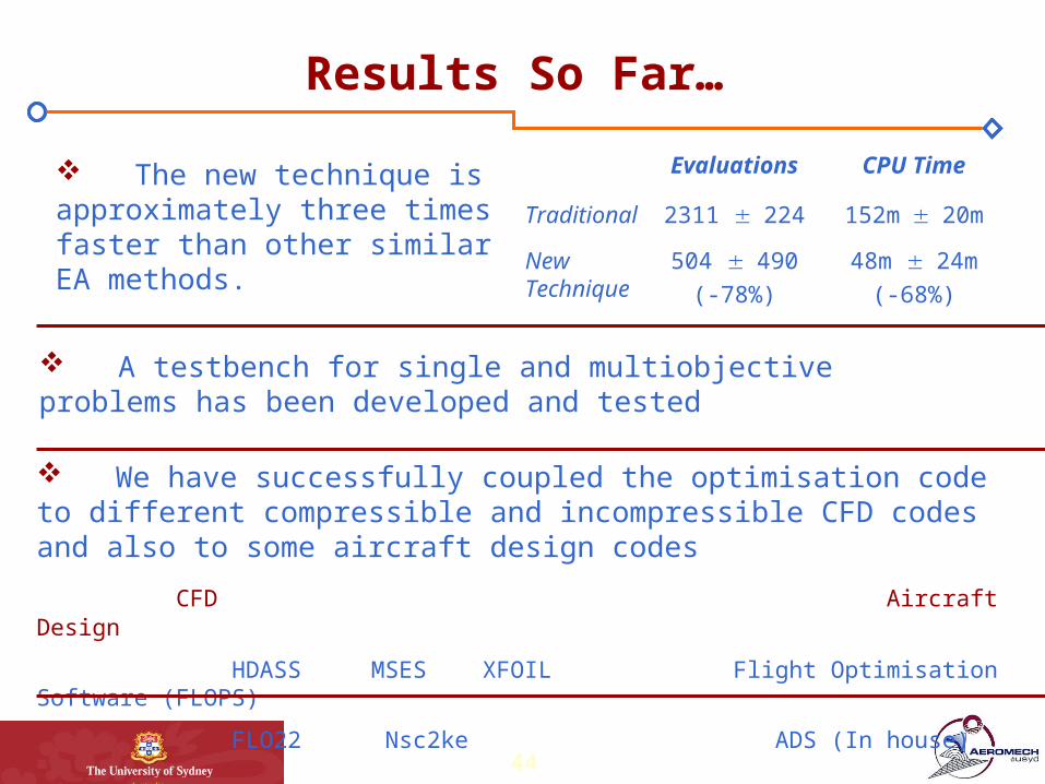
Results So Far…

Evaluations

CPU Time

Traditional

2311 224 152m20m

New Technique

504 490(-78%)

48m 24m(-68%)

The new technique is approximately three times faster than other similar EA methods.

We have successfully coupled the optimisation code to different compressible and incompressible CFD codes and also to some aircraft design codes

CFD Aircraft Design

HDASS MSES XFOIL Flight Optimisation Software (FLOPS)

FLO22 Nsc2ke ADS (In house)

A testbench for single and multiobjective problems has been developed and tested

45

Appendix-Applications

46

Publications

ADVanced EvolutioN Team (ADVENT ) Selected Publications and Conference Papers2003 E. Whitney, L. Gonzalez, K. Srinivas, J. Périaux: “Adaptive Evolution Design Without Problem Specific

Knowledge ”, Proceedings (to appear) of  EUROGEN 2003, Barcelona, Spain.2003 E. Whitney, “A Modern Evolutionary Technique for Design and Optimisation in Aeronautics ”, PhD

Thesis, School of Aerospace, Mechanical and Mechatronic Engineering, J07 University of Sydney, NSW, 2006 Australia 

2003 E. Whitney, L. Gonzalez,  J. Périaux:, and K. Srinivas, “Playing Games with Evolution: Theory and Aeronautical Optimisation Applications”,  ICIAM 2003 -- 5th International Congress on Industrial and Applied Mathematics, Sydney, Australia, July 2003. To appear. 

2002 E. Whitney, L. Gonzalez, K. Srinivas, J. Périaux: “Multi-Criteria Aerodynamic Shape Design Problems in CFD using a Modern Evolutionary Algorithm on Distributed Computers”, Proceedings of the Second International Conference on Computational Fluid Dynamics, Sydney, Australia.  

2002 J. Périaux:, M. Sefrioui, E. Whitney, L. Gonzalez, K. Srinivas, and J. Wang  “Evolutionary Algorithms, Game Theory and Hierarchical Models in CFD”, Proceedings of the Second International Conference on Computational Fluid Dynamics, Sydney, Australia.

2002 E. Whitney, M. Sefrioui, K. Srinivas, J. Périaux: “Advances in Hierarchical, Parallel Evolutionary Algorithms for Aerodynamic Shape Optimisation”, JSME (Japan Society of Mechanical Engineers) International Journal, Vol. 45, No. 1.

2001 J. Périaux, M. Sefrioui, K. Srinivas, E. Whitney, J. Wang: “Recent Advances in Evolutionary Algorithms for Multicriteria Design Optimisation in Aeronautics”, Kickoff Meeting, MACSI Working Group on Multidisciplinary Optimisation and Inverse Problems, Vienna, Austria.

2001 M. Sefrioui, E. Whitney, J. Périaux, K. Srinivas: “Evolutionary Algorithms for Multi-Objective Design Optimisation”, Proceedings of Coupling of Fluids, Structures and Waves in Aeronautics (CFSWA), A French / Australian workshop, Melbourne, Australia.

2001 J. Périaux, M. Sefrioui, K. Srinivas, E. Whitney, J. Wang: “Advances in Hierarchical Parallel Genetic Algorithms and Game Decision Strategies for Design Optimisation in Aeronautics”, Proceedings of the First French / Finnish Seminar on Innovative Methods for Advanced Technologies, Espoo, Finland.

2000 E. Whitney, K. Srinivas: “Non-Generational Multiobjective Evolution Strategy for Aerofoil Design and Optimisation Problems in CFD”: Proceedings of the First International Conference on Computational Fluid Dynamics, Kyoto, Japan:

47

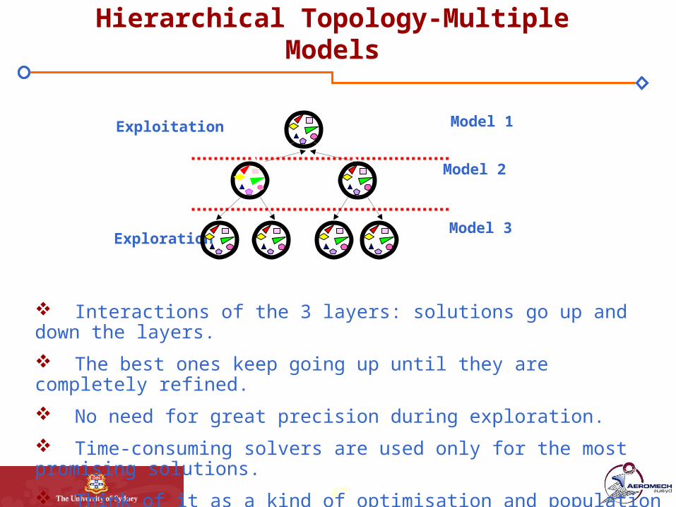
Hierarchical Topology-Multiple Models

Model 1precise model

Model 2intermediate

model

Model 3approximate

model

Exploration

Exploitation

Interactions of the 3 layers: solutions go up and down the layers.

The best ones keep going up until they are completely refined.

No need for great precision during exploration.

Time-consuming solvers are used only for the most promising solutions.

Think of it as a kind of optimisation and population based multigrid.

48

An Example: Aerofoil Optimisation

Property Flt. Cond. 1

Flt Cond.2

Mach 0.75 0.75

Reynolds 9 x 106 9 x 106

Lift 0.65 0.715

Constraints:• Thickness > 12.1% x/c (RAE 2822)• Max thickness position = 20% ® 55%

To solve this and other problems standard industrial flow solvers are being used.

Aerofoil cd

[cl = 0.65 ]

cd

[cl = 0.715 ]

Traditional Aerofoil RAE2822

0.0147 0.0185

Conventional Optimiser [Nadarajah [1]]

0.0098 (-33.3%)

0.0130 (-29.7%)

New Technique 0.0094 (-36.1%)

0.0108 (-41.6%)

For a typical 400,000 lb airliner, flying 1,400 hrs/year:

3% drag reduction corresponds to 580,000 lbs (330,000 L) less fuel burned.

[1] Nadarajah, S.; Jameson, A, " Studies of the Continuous and Discrete Adjoint Approaches to Viscous Automatic Aerodynamic Shape Optimisation," AIAA 15th Computational Fluid Dynamics Conference, AIAA-2001-2530, Anaheim, CA, June 2001.

49

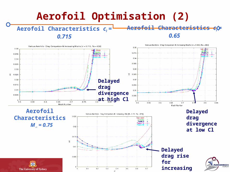
Aerofoil Characteristics cl = 0.715 Aerofoil Characteristics cl = 0.65

Delayed drag divergence at high Cl

Aerofoil Characteristics

M = 0.75

Aerofoil Optimisation (2)

Delayed drag divergence at low Cl

Delayed drag rise for increasing lift.

50

ZDT Test Cases

51

ZDT1

1 1

91: 1 +

n-1

, 1

2

1 1/

iZDT g x x

h f g f

f x x

n

i

g

52

ZDT2

1 1

92 : 1 +

n-1

, 1

22

1 1/

iZDT g x x

h f g f

f x x

n

i

g

53

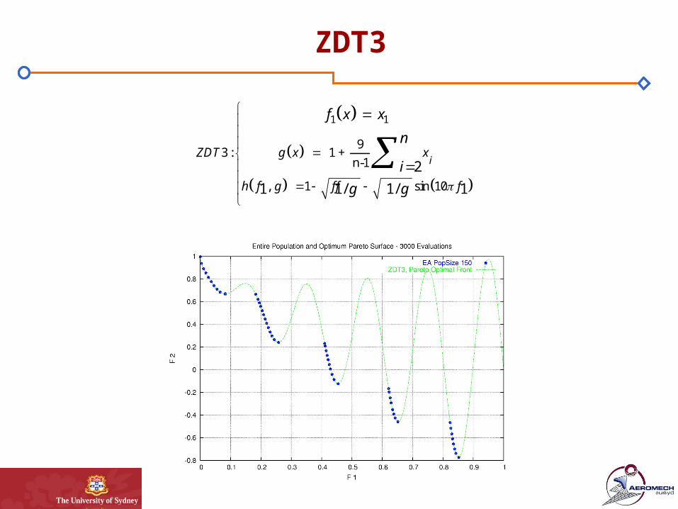
ZDT3

1 1

93 : 1 +

n-1

, 1 sin 10

2

1 1/ 1/ 1

iZDT g x x

h f g f f f

f x x

n

i

g g

54

ZDT4

1 1

4 : 1 + 10 n-1 10cos 4

, 1

2

2

1 1/

i iZDT g x x x

h f g f

f x x

n

i

g

55

Constrained Test Cases

56

BNH

4 4

5 5

5 5 25: :

8 3 7.7

0 5

0 3

2 21 1 2

2 22 1 2

2 21 1 2

2 22 1 2

12

f x x xMinimise

f x x x

C x x xBNHsubject to

C x x x

x

x

57

SRN

2+ 2 1

9 1

: 225 :

3 10 0

20 20,

20 20

2 21 1 2

22 1 2

2 21 1 2

2 1 2

12

f x x xMinimise

f x x x

SRN C x x xsubject to

C x x x

x

x

58

, 16 1 max( )

: : max 1(10

1 3,

0

2 21 1 2

2 AC, BC5)

AC, BC

f x y x y x yMinimisef x

TwoBarTrusssubject to

y

x

Two Bar Truss Design

A B

1x 2x

59

Goal Programming- Test Problem P1

, 2

, 2

: 0.1 1,0 101:

10

10 5

10

1 1 2

2 1 2

1 2

1 12

22

1

f x xMinimise

f x x

subject to S x xP

f x

xf

x

60

Results. Candidate and Target Geometries

61

Results: Example of Convergence.

Mesh Adaptation : Mesh 15