1 minimum message length inference and parameter...
TRANSCRIPT
1
Minimum Message Length Inference and
Parameter Estimation of Autoregressive and
Moving Average ModelsDaniel F. Schmidt
Abstract
This technical report presents a formulation of the parameter estimation and model selection problem
for Autoregressive (AR) and Moving Average (MA) models in the Minimum Message Length (MML)
framework. In particular, it examines suitable priors for both classes of models, and subsequently derives
message length expressions based on the MML87 approximation. Empirical results demonstrate the new
MML estimators outperform several benchmark parameter estimation and model selection criteria on
various prediction metrics.
Daniel Schmidt is with Monash University
Clayton School of Information Technology
Clayton Campus Victoria 3800, Australia
Telephone: +61 3 9905 3414, Fax: +61 3 9905 5146
Email: [email protected]
2
CONTENTS
I Introduction 5
II Literature Review 5
II-A Problem Statement . . . . . . . . . . . . . . . . . . . . . . . . . . . . . . . . . . . 5
II-A.1 Stationarity and Invertibility . . . . . . . . . . . . . . . . . . . . . . . . 6
II-B Auto-Regressive Parameter Estimation . . . . . . . . . . . . . . . . . . . . . . . . . 6
II-B.1 Unconstrained Least Squares . . . . . . . . . . . . . . . . . . . . . . . . 6
II-B.2 Maximum Likelihood . . . . . . . . . . . . . . . . . . . . . . . . . . . . 6
II-B.3 Yule-Walker . . . . . . . . . . . . . . . . . . . . . . . . . . . . . . . . . 6
II-B.4 Burg . . . . . . . . . . . . . . . . . . . . . . . . . . . . . . . . . . . . . 6
II-C Moving Average Parameter Estimation . . . . . . . . . . . . . . . . . . . . . . . . . 6
II-D Methods for Order Selection . . . . . . . . . . . . . . . . . . . . . . . . . . . . . . 7
II-E The Minimum Message Length criterion . . . . . . . . . . . . . . . . . . . . . . . . 7
III General Parameter Priors for LTI AR and MA models 9
III-A Full Prior Density . . . . . . . . . . . . . . . . . . . . . . . . . . . . . . . . . . . . 10
III-B Priors for β . . . . . . . . . . . . . . . . . . . . . . . . . . . . . . . . . . . . . . . 10
III-B.1 Priors on Real Poles . . . . . . . . . . . . . . . . . . . . . . . . . . . . . 10
III-B.2 Prior Correction for the Reference Prior . . . . . . . . . . . . . . . . . 13
III-B.3 Priors on Complex Pole Pairs . . . . . . . . . . . . . . . . . . . . . . . 13
III-C Priors for c . . . . . . . . . . . . . . . . . . . . . . . . . . . . . . . . . . . . . . . . 14
III-D Priors for σ2 . . . . . . . . . . . . . . . . . . . . . . . . . . . . . . . . . . . . . . . 15
III-E Priors for Model Structure . . . . . . . . . . . . . . . . . . . . . . . . . . . . . . . 15
IV Auto-regressive (AR) Models 16
IV-A Likelihood Function . . . . . . . . . . . . . . . . . . . . . . . . . . . . . . . . . . . 17
IV-B The Fisher Information Matrix . . . . . . . . . . . . . . . . . . . . . . . . . . . . . 18
IV-C Unconditional Likelihood Information Matrix . . . . . . . . . . . . . . . . . . . . . 18
IV-D Conditional Likelihood Information Matrix . . . . . . . . . . . . . . . . . . . . . . 19
IV-E Fisher Information Matrix Algorithm . . . . . . . . . . . . . . . . . . . . . . . . . 20
IV-F Parameter Estimation . . . . . . . . . . . . . . . . . . . . . . . . . . . . . . . . . . 21
IV-F.1 Maximum Likelihood Estimate of σ2 . . . . . . . . . . . . . . . . . . . 21
3
IV-F.2 Minimum Message Length Estimate of σ2 . . . . . . . . . . . . . . . . 22
IV-F.3 Minimum Message Length Estimate of β . . . . . . . . . . . . . . . . . 23
IV-F.4 Derivatives of the Message Length . . . . . . . . . . . . . . . . . . . . . 24
IV-F.5 A Quick Note on Numerical Issues with the Search . . . . . . . . . . . 25
IV-G Remarks on the MML87 AR Estimator . . . . . . . . . . . . . . . . . . . . . . . . 25
IV-G.1 The Effect of σ2 on the Parameter Accuracy . . . . . . . . . . . . . . . 25
IV-G.2 The Effect of the FIM on the β-parameter Estimates . . . . . . . . . . . 25
IV-G.3 The AR(1) Estimator of αMML for the Reference Prior . . . . . . . . . 26
V Moving Average (MA) Models 26
V-A Likelihood Function . . . . . . . . . . . . . . . . . . . . . . . . . . . . . . . . . . . 27
V-B The Fisher Information Matrix . . . . . . . . . . . . . . . . . . . . . . . . . . . . . 27
V-C Parameter Estimation . . . . . . . . . . . . . . . . . . . . . . . . . . . . . . . . . . 29
V-C.1 Maximum Likelihood Estimation of the Noise Variance . . . . . . . . . 29
V-C.2 Minimum Message Length Estimation of the Noise Variance . . . . . . 29
V-C.3 Minimum Message Length Estimation of c . . . . . . . . . . . . . . . . 30
V-C.4 The CLMML Estimator . . . . . . . . . . . . . . . . . . . . . . . . . . . 30
V-D Remarks on the MML87 MA Estimator . . . . . . . . . . . . . . . . . . . . . . . . 31
VI Experimental Results 32
VI-A Experimental Design . . . . . . . . . . . . . . . . . . . . . . . . . . . . . . . . . . 32
VI-A.1 Parameter Estimation Experiments . . . . . . . . . . . . . . . . . . . . . 32
VI-A.2 Order Selection Experiments . . . . . . . . . . . . . . . . . . . . . . . . 32
VI-A.3 Experiments on Real Data . . . . . . . . . . . . . . . . . . . . . . . . . 32
VI-B Alternative Criteria . . . . . . . . . . . . . . . . . . . . . . . . . . . . . . . . . . . 33
VI-C Evaluation of Results . . . . . . . . . . . . . . . . . . . . . . . . . . . . . . . . . . 34
VI-C.1 Squared Prediction Error . . . . . . . . . . . . . . . . . . . . . . . . . . 34
VI-C.2 Negative Log-Likelihood and KL-Divergence . . . . . . . . . . . . . . . 35
VI-C.3 Order Selection . . . . . . . . . . . . . . . . . . . . . . . . . . . . . . . 36
VI-D Autoregressive Experiments . . . . . . . . . . . . . . . . . . . . . . . . . . . . . . . 36
VI-D.1 Parameter Estimation Experiments . . . . . . . . . . . . . . . . . . . . . 36
VI-D.2 Order Selection Experiments . . . . . . . . . . . . . . . . . . . . . . . . 37
VI-D.3 Experiments on Real Data . . . . . . . . . . . . . . . . . . . . . . . . . 37

4
VI-E Moving Average Experiments . . . . . . . . . . . . . . . . . . . . . . . . . . . . . 37
VI-E.1 Parameter Estimation Experiments . . . . . . . . . . . . . . . . . . . . . 37
VI-E.2 Order Selection Experiments . . . . . . . . . . . . . . . . . . . . . . . . 37
VII Discussion of Results 38
VII-A Autoregressive Parameter Estimation Results . . . . . . . . . . . . . . . . . . . . . 38
VII-B Autoregressive Order Selection Results . . . . . . . . . . . . . . . . . . . . . . . . 40
VII-C Autoregressive Order Selection on Real Data . . . . . . . . . . . . . . . . . . . . . 41
VII-D Moving Average Parameter Estimation Results . . . . . . . . . . . . . . . . . . . . 42
VII-E Moving Average Order Selection Results . . . . . . . . . . . . . . . . . . . . . . . 44
VIII Conclusion 53
Appendix I: A Curved Prior Correction Modification 53
Appendix II: Autoregressive Moving-Average Models 53
Appendix III: Computing Autoregressive Moving-Average Likelihoods via the Kalman Filter 56
References 57

5
I. INTRODUCTION
The Autoregressive (AR) and Moving Average (MA) models [1] are heavily studied and widely used
methods of analysing time correlated data, commonly referred to as time series. The two issues of
estimating suitable parameters for an AR or MA model given a particular structure, and of estimating
the structure of the models are also well studied with many methods in existence. This tech report
presents new estimators for the parameters and structure of both AR and MA models based on the
Minimum Message Length criterion [2], and empirical results demonstrate the effectiveness of these
methods over conventional and benchmark techniques. This document is organised as follows: Section II
examines previous work on the topic of parameter estimation and order selection for AR and MA models,
Section III discusses suitable prior densities/distributions for AR and MA parameters, Section IV and V
cover the formulation of the AR and MA models in the MML87 framework, Section VI describes the
experimental design and suitable test metrics, and Section VII examines and discusses the experimental
results. The Appendices provide some additional information: Appendix I details the new Curved Prior
Modification to MML87 that is used in this work and Appendix II presents some preliminary work on
mixed Autoregressive Moving Average (ARMA) models within an MML87 framework. Appendix III
summarises the Kalman Filtering approach to efficiently computing the likelihood of ARMA processes,
including a suitable initialisation scheme; this has been included primarily for convenience.
II. LITERATURE REVIEW
A. Problem Statement
Given a sequence of observed, time ordered data y = [y1, ..., yN ], the AR(P) (P -th order autoregressive
model) explanation is given by
yn +P∑
i=1
aiyn−i = vn (1)
where a are the autoregressive coefficients, and v = [v1, ..., vN ] is a vector of unobserved innovations,
distributed as per vn ∼ N (0, σ2) where σ2 is the innovation variance. The MA(Q) (Q-th order moving
average model) explanation for the same data is given by
yn =
Q∑
i=1
civn−i + vn (2)
where c is the vector of moving average parameters, and once again v is the Normally distributed
innovation sequence. The task considered in the sequel is estimation of P , a and σ2 from y for the AR
explanation, and estimation of Q, c and σ2 from y for the MA explanation. This tech report does not
examine Autoregressive Moving Average (ARMA) beyond some brief results in Appendix II.
6
1) Stationarity and Invertibility: The time response of an AR model can be studied by examining the
roots of its characteristic polynomial. This polynomial is formed as
A(D) = 1 +
P∑
i=1
aiD−i (3)
where D is the delay operator, i.e. ynD−i = yn−i. The roots, p, of A(D) are known as the system
poles, and their location determines the dynamic response of the model. In particular, an AR process is
stable, and consequently stationary, if and only if all the roots lie within the unit circle [1]. A similar
condition applies to Moving Average models; in this case, if the roots, or zeros, of C(q) lie within the
unit circle, the MA process is termed invertible. All AR and MA models considered in this technical
report are assumed to be stationary and invertible.
B. Auto-Regressive Parameter Estimation
The task of estimating the autoregressive coefficients, a, from a time series is a well studied problem.
Over the years there have been a great many different methods proposed, and a few of the most common
and widely used are examined next.
1) Unconstrained Least Squares: While being a simple scheme, it suffers from giving no guarantees
on the stationarity (and thus, stability) of the resultant estimates. For any purpose beyond one step ahead
prediction, these estimates are therefore worthless if it is assumed the data is stationary [1].
2) Maximum Likelihood: : The Maximum Likelihood estimates are found by maximising the complete
negative log-likelihood. It possesses well known asymptotic properties, and guarantees stable estimates,
but suffers from being difficult to compute. Generally the estimates are found by a numerical search [3].
3) Yule-Walker: : The Yule-Walker estimator is a method-of-moments estimation scheme that works
by estimating the model coefficients from the sample autocovariances, and produces models that are
guaranteed to be stable. [1].
4) Burg: : The Burg estimator works by minimising forward and backward prediction errors. It is fast,
guarantees stable models and performs very well [4].
C. Moving Average Parameter Estimation
For parameter estimation of Moving Average processes there are also several estimation schemes
commonly encountered in the literature, the most popular being the Maximum Likelihood estimator, and
those techniques based on Prediction Error Methods (PEM) [5]. The Maximum Likelihood estimates
guarantee invertibility, but are slow to find and involve non-linear optimisation. There are many methods

7
based on prediction errors and model inversion [6], [7], but these can give poor performances in the face
of short data sequences as compared to the Maximum Likelihood estimates.
D. Methods for Order Selection
The estimation of P and Q for AR and MA processes is also a widely studied problem with many
proposed solutions. Amongst the most common methods for order selection are those based on model
parsimony - that is, methods that punish complexity and attempt to find a trade-off between model
complexity and capability in an attempt to improve the generalisation capabilities of the selected model.
One of the earliest of these methods was the work by Wallace and Boulton in 1968 [8] on Mixture
Modelling, which later led to the development of the MML criterion and its subsequent family of
approximations. Other pioneering work on model selection by parsimony includes the AIC criterion
[9], developed for automatic order selection of AR processes. Further refinements of the AIC scheme
for short time series led to the development of the AICc (corrected AIC) [10] estimator. Similar work
has led to the Bayesian Information Criteria (BIC) [11], and more recently, the symmetric Kullback-
Leibler distance Information Criteria (KIC) [12] and the corrected variant (KICc) [13]. An alternative to
the MML criterion has been the Minimum Description Length (MDL) criterion pioneered by Rissanen.
Early versions of MDL [14] yield criterion similar to BIC for many models, but the latest developments
have led to the modern Normalised Maximum Likelihood (NML) [15] criterion. While there are other
methods for model selection of AR and MA models, such as those based on predictive least squares [16],
[17], variations of Information Criteria [18], and Bayesian techniques [19], this document compares the
MML criterion to the most common techniques used in the literature.
E. The Minimum Message Length criterion
The Minimum Message Length criterion [2], [20], [21] is a unified framework for inference of model
structure and parameters, based on Information Theoretic arguments. The basic concept is that of a sender
wishing to transmit a sequence of data to a receiver across a noiseless communication channel. The sender
does so by first stating the model they shall use to encode the data (the assertion), and then sending the
data given this model (the detail). The model that yields the shortest message length is considered to be
the best model that can be inferred from the data, and is a tradeoff between complexity of the model
(the assertion) and goodness of fit (the detail). As has been previously mentioned, the seminal work by
Wallace and Boulton [8] is the genesis of the entire MML concept. The subsequent SMML criterion [20],
which is the theoretical basis for all the practical MML approximations, works by dividing a countable

8
set of possible data into regions, each with an associated point estimate. This division is performed so
as to minimise the expected message length of a random datum drawn from the marginal distribution
of all data. Although this scheme has many strong properties, it suffers from the NP-hard nature of the
region construction [22] and is thus untenable in practice. To this end a range of MML approximations
have been proposed, the most popular undoubtedly being the MML87 estimator [21]. This method works
by constructing the model codebook using the prior distribution instead of the marginal distribution, and
estimating the volume of the coding region on which the model codeword is based. Under assumptions
that the model priors are locally approximately ‘flat’, and the expected negative log-likelihood surface is
locally approximately quadratic, the estimated message length of some data y and a model θ is given by
I(y,θ) = − log h(θ) +1
2log |J(θ)| − log f(y|θ) + κ(dim (θ)) (4)
where f(y|θ) is the likelihood function, h(·) is the prior distribution over the model parameters, J(·) is
the Fisher Information Matrix and κ(·) is a constant introduced through the approximation that depends
only on the number of model parameters. Inference in an MML87 framework is performed by seeking
the model that minimises (4). Alternatives to MML87 do exist, amongst them the MMLD approximation
[23] which seeks a region in parameter space, but involves the evaluation of complex integrals. The
MMLD MMC [23] algorithm uses importance sampling to construct the region and compute the integral
simultaneously, and provides an alternative to (4) that operates under relaxed assumptions, but is naturally
slower as there is a large amount of sampling involved. This document presents estimators for the AR
and MA model classes that are based on the MML87 estimator.
9
III. GENERAL PARAMETER PRIORS FOR LTI AR AND MA MODELS
Inference in a Minimum Message Length framework involves making a statement about the posterior
distribution of a model. Therefore, it is a requirement of the MML87 criterion that prior densities over all
model parameters be fully specified. In this section a set of useful priors for the parameters in the ARMA
family of models is examined. It begins with a discussion of suitable priors by briefly re-examining the
ARMA model structure. The variety of ARMA model this work details has the autoregressive components
described in root-space (as per [24]), and the moving average components described in coefficient space,
i.e. the ARMA(P, Q) explanation for a series y is given byP∏
i=1
(1−D−1pi)yn =
R∑
i=1
civn−i + vn (5)
where c are the moving average parameters, v is the i.i.d. Normally distributed innovation sequence, D
is the delay operator, and p are the roots (poles) of the ARMA model’s characteristic polynomial (given
by the autoregressive coefficients). The AR and MA models may be formed from the general ARMA
structure by setting either Q = 0 for an AR model, or P = 0 for an MA model. For any polynomial
with strictly real coefficients, all roots must either be wholly real, i.e. pi = αi, or complex conjugate
pairs of the form pi,j = ri exp (jωi) , ri exp (−jωi). Thus, the vector of poles p is a function of what
is termed the root parameters, and the autoregressive coefficients are a function of the poles, that is
p ≡ p(α, r,ω) ≡ p(β) (6)
a′ ≡ poly (p(β)) (7)
a = a′(2:P+1) (8)
where β = α, r,ω is now the complete collection of root parameters. This of course has the conse-
quence of complicating the resulting model’s Fisher Information Matrix significantly; there are however,
several key advantages to using this representation of the model that justify the extra work:
1) The ARMA model’s time response is determined largely by the poles of the model. The autore-
gressive coefficient parameters do not have an intuitive time-response interpretation and thus it is
difficult to select suitable priors for these parameters. In contrast, the root-parameters have a direct
effect on the time response of the model.
2) This structure allows ARMA models to be examined based on their underlying structural compo-
nents. In coefficient space, an AR(P) process is a single model class; a root-space representation
allows an AR(P) process to be broken into (P/2+1) different processes by examining the different
combinations of root structure allowed with P delays.

10
With these advantages in mind, suitable priors for our ARMA model parameters are now examined.
A. Full Prior Density
The full prior density over a complete ARMA model is examined first, i.e. θ =
P,Q,β, c, σ2
. By
assuming some degree of statistical independence between parameters, the total prior density h(θ) can
be factorised into the following products
h(θ) = h(P ) · h(Q) · h(β) · h(c) · h(σ2) (9)
With this specification it is easy to see that the total prior density can be modified for subset ARMA models
by merely removing the appropriate parameters. Suitable priors for all parameters in θ are examined in
the next subsections.
B. Priors for β
Priors for the autoregressive root-space parameters β are examined first. Begin by recalling that for
an AR model to be stationary all of its poles p must like within the perimeter of the unit circle centred
at D = 0. A simple prior would then be to make h(p) ∝ 1 on the unit circle. However, it should be
recalled that poles only come in two flavours: wholly real poles, and complex conjugate pole pairs, and
the moduli and radii of these poles help to determine the time response of the AR model. Priors for both
types of parameters are now discussed.
1) Priors on Real Poles: For a purely real pole, pi = αi and thus |pi| = |αi| and clearly ∠pi = 0;
thus a prior density is required only on the real component of pi. The effect of a particular prior density
upon our inferences can be roughly determined by examining the time response of AR(1) model, i.e. an
autoregressive model with a single real pole. The impulse response of an unforced AR(1) model with
real pole at α is given exactly by
yn = αn, n ∈ Z, n ≥ 0 (10)
This sequence may be exactly produced by sampling the continuous time process
yt = exp
(
− t
τ
)
(11)
at uniform intervals t = 0, 1, 2, ...,∞, where τ is the time constant of the process. The relation between
α and τ is given by
τ = − 1
logα(12)

11
This nonlinear relationship indicates that as α→ 1 the range of different time responses as characterised
by their time constants becomes denser. As the AR model is designed to model time series data, and
thus time responses, it is helpful to view the model parameters in terms of this time constant. For some
prior distribution h(α), the resulting induced density on τ can be found by
h(τ) =d
dτ
exp
(
−1
τ
)
· h(
α|α = exp
(
−1
τ
))
(13)
=
exp
(
−1
τ
)
τ2· h(
α|α = exp
(
−1
τ
))
(14)
Several candidate priors for α are now considered, and the resultant induced prior density on τ observed
using (14). Over the course of many years of Bayesian analysis of autoregressive processes a wide range
of possible priors have been proposed; a subset of popular choices is examined next:
hu(α) =1
2(15)
hr(α) =1
π√
(1− α2)(16)
hb(α|a, b) =1
2B(a, b)|α|a−1(1− |α|)b−1 (17)
hn(α|σ2α) =
√2 exp
(
−1
2log
(
−α+ 1
α− 1
)2
σ−2α
)
(√πσα|α2 − 1|
)−1(18)
hp(α|T ) =
(
(1− α2)−1
(
T − 1− α2T
1− α2
))
1
2
· Ω(T )−1 =P(α|T )
Ω(T )(19)
with all distributions defined on the support α ∈ (−1, 1), i.e. the stationarity region. A discussion of
these priors follows:
1) Uniform Prior: The prior in (15) is clearly the uniform prior. While this is a traditionally ‘unin-
formative’ prior, it be observed from its induced prior on τ that it puts very little probability mass
on τ > 4, which can lead it to favour models with faster poles.
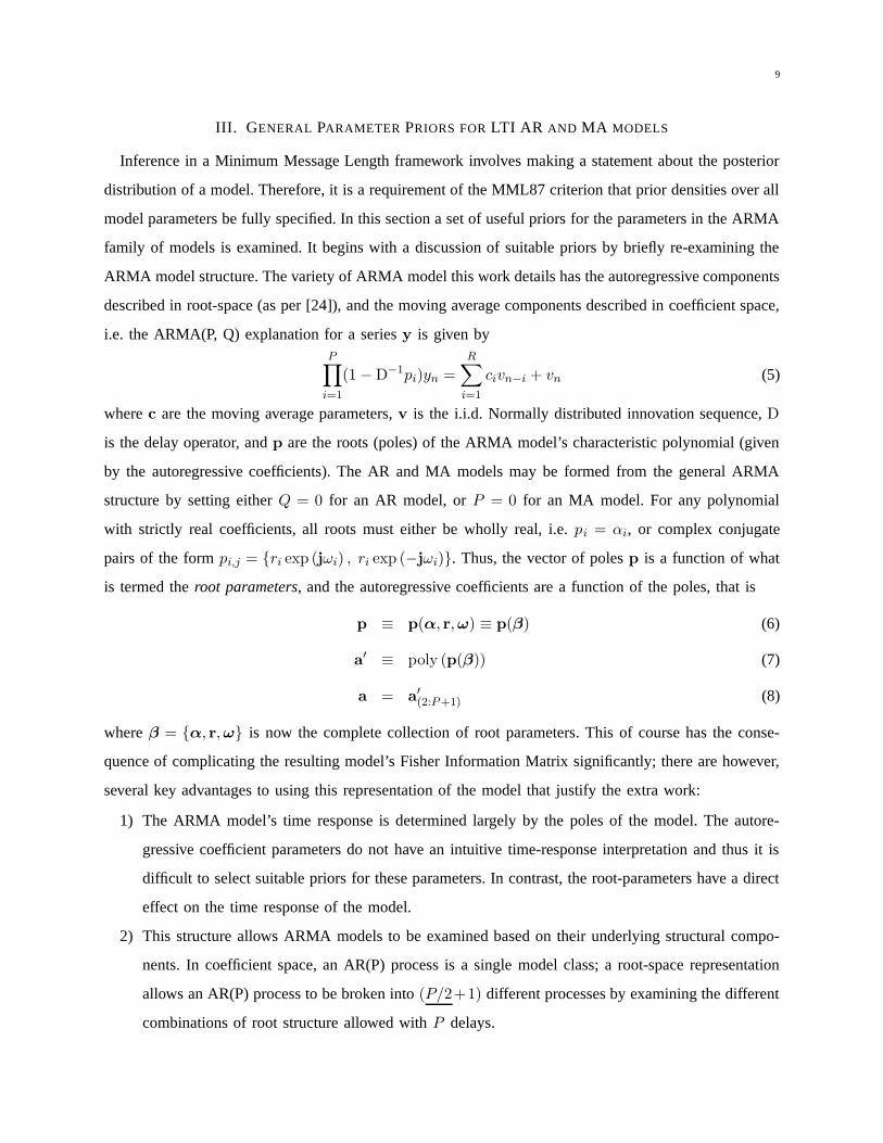
2) Reference Prior: The prior given by (16) is the Yang and Berger [25] reference prior and is shown
in α-space in Figure 1(a); for AR(1) models it is also a Jeffrey’s prior. Figure 1(b) shows that it
places more mass for τ > 4 and is thus significantly less biased towards faster models than the
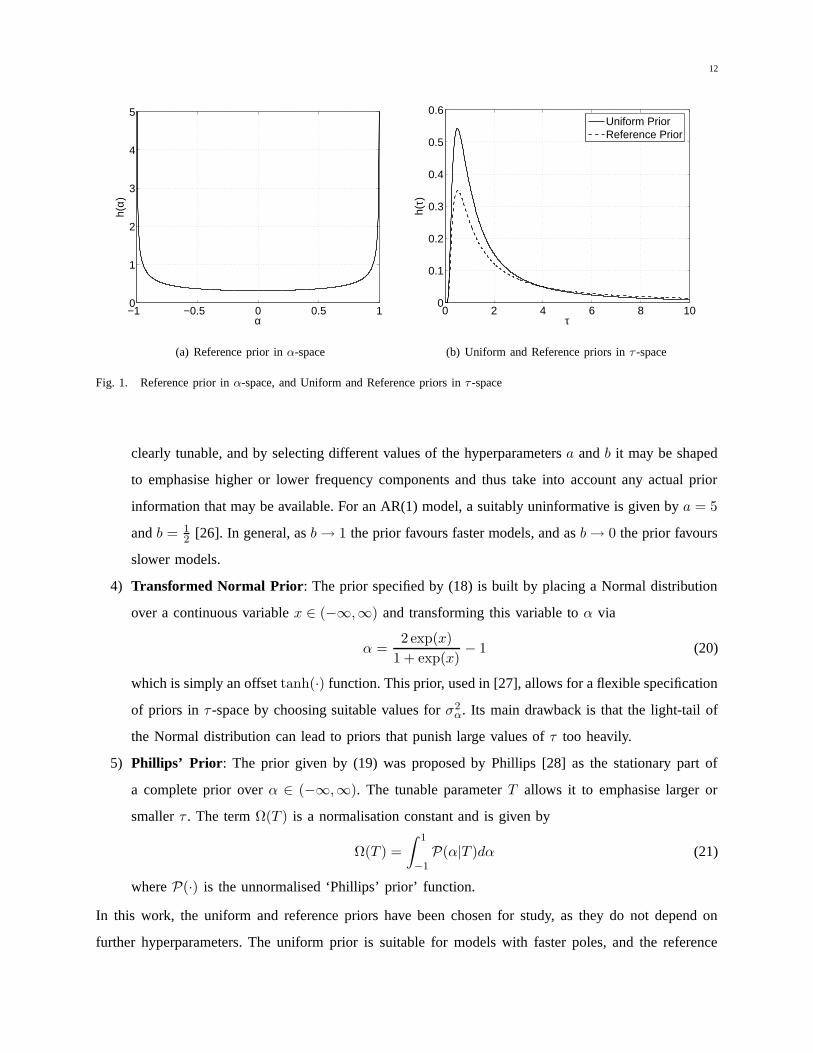
uniform prior. This is clear from the plot of the ratio of uniform prior on reference prior in τ -space
given in Figure 2. For values of τ > 4 the reference prior assigns significantly higher proportion
of probability mass than does the uniform prior.
3) Beta Prior: The prior specified by (17) is a Beta prior on the modulus of α; the scaling by 12
takes into account the sign of α, giving positive and negative values equal weighting. This prior is
12
−1 −0.5 0 0.5 10
1
2
3
4
5
α
h(α)
(a) Reference prior in α-space
0 2 4 6 8 100
0.1
0.2
0.3
0.4
0.5
0.6
τ
h(τ)
Uniform PriorReference Prior
(b) Uniform and Reference priors in τ -space
Fig. 1. Reference prior in α-space, and Uniform and Reference priors in τ -space
clearly tunable, and by selecting different values of the hyperparameters a and b it may be shaped
to emphasise higher or lower frequency components and thus take into account any actual prior
information that may be available. For an AR(1) model, a suitably uninformative is given by a = 5
and b = 12 [26]. In general, as b→ 1 the prior favours faster models, and as b→ 0 the prior favours
slower models.
4) Transformed Normal Prior: The prior specified by (18) is built by placing a Normal distribution
over a continuous variable x ∈ (−∞,∞) and transforming this variable to α via
α =2 exp(x)
1 + exp(x)− 1 (20)
which is simply an offset tanh(·) function. This prior, used in [27], allows for a flexible specification
of priors in τ -space by choosing suitable values for σ2α. Its main drawback is that the light-tail of
the Normal distribution can lead to priors that punish large values of τ too heavily.
5) Phillips’ Prior: The prior given by (19) was proposed by Phillips [28] as the stationary part of
a complete prior over α ∈ (−∞,∞). The tunable parameter T allows it to emphasise larger or
smaller τ . The term Ω(T ) is a normalisation constant and is given by
Ω(T ) =
∫ 1
−1P(α|T )dα (21)
where P(·) is the unnormalised ‘Phillips’ prior’ function.
In this work, the uniform and reference priors have been chosen for study, as they do not depend on
further hyperparameters. The uniform prior is suitable for models with faster poles, and the reference
13
0 20 40 60 80 1000
0.2
0.4
0.6
0.8
1
1.2
1.4
1.6
τ
h u(τ)
/ hr(τ
)
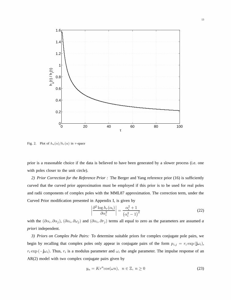
Fig. 2. Plot of hu(α)/hr(α) in τ -space
prior is a reasonable choice if the data is believed to have been generated by a slower process (i.e. one
with poles closer to the unit circle).
2) Prior Correction for the Reference Prior : The Berger and Yang reference prior (16) is sufficiently
curved that the curved prior approximation must be employed if this prior is to be used for real poles
and radii components of complex poles with the MML87 approximation. The correction term, under the
Curved Prior modification presented in Appendix I, is given by∣
∣
∣
∣
∂2 log hr(αi)
∂α2i
∣
∣
∣
∣
=α2
i + 1(
α2i − 1
)2 (22)
with the (∂αi, ∂αj), (∂αi, ∂ωj) and (∂αi, ∂rj) terms all equal to zero as the parameters are assumed a
priori independent.
3) Priors on Complex Pole Pairs: To determine suitable priors for complex conjugate pole pairs, we
begin by recalling that complex poles only appear in conjugate pairs of the form pi,j = ri exp (jωi),
ri exp (−jωi). Thus, ri is a modulus parameter and ωi the angle parameter. The impulse response of an
AR(2) model with two complex conjugate pairs given by
yn = Krncos(ωn), n ∈ Z, n ≥ 0 (23)
14
It can be observed then that the r parameter has a similar effect on the time response to the α parameter
in a real pole, and thus a similar prior may be appropriate. One choice of prior on ω is to make it uniform
on ω ∈ [0, π], i.e. the range of normalised frequencies a discrete system may assume [27]. Another option
is the ‘component reference prior’, which is formed by taking a uniform prior over the coefficients of an
AR(2) model with complex poles [24]. This prior, which biases away from models with extremely high
or low frequency components leads to the prior for a complete complex pair given by
h(r, ω) = 2h(|r|) ·(
1
2sinω
)
= h(|r|) sinω (24)
where h(|r|) is selected from the previous section, i.e. from priors (15)-(19). The prior is scaled by a
factor of two to account for the fact that r ∈ (0, 1), whereas the priors on real poles are defined on the
support (−1, 1). For the experiments presented later in this tech report, the prior given by (24) was used,
with either the uniform or reference taken over h(|r|).
C. Priors for c
The starting point for specifying priors over the moving average coefficients is to make the assumption
that the model is invertible. From this it follows that the roots of C(q) must be constrained to lie within
the unit circle. As the likelihoods of the models presented in the sequel are parametrised in moving
average coefficient space it is certainly valid to choose priors over the parameter polynomial C(q) rather
than its roots. Given no prior knowledge on the values of the parameters, other than the requirement they
are invertible, a suitable choice is the uniform prior over the valid region of values the vector c may
assume, that is
h(c) =1
vol(
Λdim(c)
) (25)
where Λk is the hyper-region of k-ary polynomial parameters for which all roots are within the unit
circle, i.e.
Λk =
C(q) ∈ Rk : |roots(C(q))|∞ < 1
(26)
and vol(x) is the volume of the hyper-region x. A method of computing the volume of the region Λk is
given by [30] and is summarised below for completeness
Mk+1 =k
k + 1Mk−1, M1 = 2 (27)
vol (Λk) = (M1 ·M3 ·M5 · ...Mk−1)2 , if k is even (28)
vol (Λk+1) = vol (Λk)Mk+1 (29)

15
TABLE I
ENUMERATIONS OF POLE STRUCTURES FOR THE AR(P) MODELS FOR P = 1 . . . 4
S P PR PC β
1 1 1 0 α1
2 2 2 0 α1, α2
3 2 0 2 r1, ω1
4 3 3 0 α1, α2, α3
5 3 1 2 α1, r1, ω1
6 4 4 0 α1, α2, α3, α4
7 4 2 2 α1, α2, r1, ω1
8 4 0 4 r1, ω1, r2, ω2
This prior, uniform over the coefficient space is the same as previously used by Fitzgibbon [31] and Sak
[32] with success.
D. Priors for σ2
A very common choice of prior that has been widely used for model variance σ2 is the scale invariant
prior [2]. This prior is designed by placing a uniform prior on log σ2; appropriate transformation of
h(log σ2) to h(σ2) yieldsd
dσ2
log σ2
· 1 =1
σ2(30)
This prior is clearly improper, and can be rendered proper by using a suitable normalisation over an
appropriate support. The final scale-invariant prior on σ2 is then given by
h(σ2) =1
σ2· 1
log(σ2U )− log(σ2
L), σ2 ∈ [σ2
L, σ2U ] (31)
This prior is used for all experiments in this technical report. The inverse-gamma [27] is another possible
prior for σ2, though using this does not lead to as simple MML estimators as the above scale invariant
prior.
E. Priors for Model Structure
One possible prior for the autoregressive structure is to select a maximum number of poles that
is considered reasonable (the maximum ‘order’ of the AR model) and the enumerate all possible β-
structures models in this range may assume. Placing a uniform distribution on all enumerations allows
for an equal a priori belief on any individual structure being chosen. For an AR(P) model, there are
16
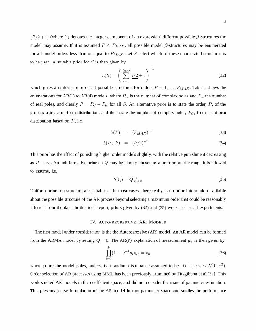
(P/2 +1) (where (·) denotes the integer component of an expression) different possible β-structures the
model may assume. If it is assumed P ≤ PMAX , all possible model β-structures may be enumerated
for all model orders less than or equal to PMAX . Let S select which of these enumerated structures is
to be used. A suitable prior for S is then given by
h(S) =
(
PMAX∑
i=1
i/2 + 1
)−1
(32)
which gives a uniform prior on all possible structures for orders P = 1, . . . , PMAX . Table I shows the
enumerations for AR(1) to AR(4) models, where PC is the number of complex poles and PR the number
of real poles, and clearly P = PC + PR for all S. An alternative prior is to state the order, P , of the
process using a uniform distribution, and then state the number of complex poles, PC , from a uniform
distribution based on P , i.e.
h(P ) = (PMAX)−1 (33)
h(PC |P ) = (P/2)−1 (34)
This prior has the effect of punishing higher order models slightly, with the relative punishment decreasing
as P →∞. An uninformative prior on Q may be simply chosen as a uniform on the range it is allowed
to assume, i.e.
h(Q) = Q−1MAX (35)
Uniform priors on structure are suitable as in most cases, there really is no prior information available
about the possible structure of the AR process beyond selecting a maximum order that could be reasonably
inferred from the data. In this tech report, priors given by (32) and (35) were used in all experiments.
IV. AUTO-REGRESSIVE (AR) MODELS
The first model under consideration is the the Autoregressive (AR) model. An AR model can be formed
from the ARMA model by setting Q = 0. The AR(P) explanation of measurement yn is then given by
P∏
i=1
(1−D−1pi)yn = vn (36)
where p are the model poles, and vn is a random disturbance assumed to be i.i.d. as vn ∼ N (0, σ2).
Order selection of AR processes using MML has been previously examined by Fitzgibbon et al [31]. This
work studied AR models in the coefficient space, and did not consider the issue of parameter estimation.
This presents a new formulation of the AR model in root-parameter space and studies the performance

17
of the resultant MML estimator in terms of both order selection and autoregressive parameter estimation.
The total prior probability density over the AR model is given by
h(θ) = h(P ) · h(β) · h(σ2) (37)
where the priors are chosen as per Section (III).
A. Likelihood Function
The most straightforward way of modelling the data given an autoregressive model is through the
unconditional negative log-likelihood, i.e.
L(y|θ) =N
2log(2π) +
1
2log |W(θ)| + 1
2yW−1(θ)yT (38)
where W(θ) = Ey
[
yTy]
is the (N ×N) theoretical covariance matrix of data given an autoregressive
model. This expression involves inversions of large matrices which, while being simplified by the Kalman
Recursions [42], is unnecessarily complex. An alternative expression to (38) is based on the conditional
likelihood. From an examination of (36) it is obvious that the likelihood of a measurement in the sequence
y is conditional on the P previous measurements. Thus, the modelling error between yn and the predicted
value of yn conditioned on the previous P samples of y is given by
zn = yn +
P∑
k=1
akyn−k (39)
It is thus possible to rewrite the negative log-likelihood as
L(y|θ) =P
2log(2π) +
1
2log |Γ(θ)|+ 1
2y(1:P )Γ
−1(θ)yT(1:P )
+N − P
2
(
log(2π) + log σ2)
+1
2σ2
N∑
n=P+1
z2n (40)
where Γ(θ) is the P ×P theoretical autocovariance matrix used to model the first P measurements of y
for which no conditional means may be computed. As (39) is simply a linear regression, the expression
may be rewritten more compactly in matrix notation by defining xn = [yn−1, . . . , yn−P ], and then building
the autoregression matrix
Φ =[
xT(P+1), . . . ,x
TN
]
(41)
The negative log-likelihood may then be written as
L(y|θ) =N
2log(2π) +
1
2log (|Γ(θ)|) +
1
2y(1:P )Γ
−1(θ)yT(1:P ) (42)
+N − P
2log(σ2) +
1
2σ2
(
y(P+1:N) + aΦ) (
y(P+1:N) + aΦ)T −N log ε
where ε is the measurement accuracy of the data
18
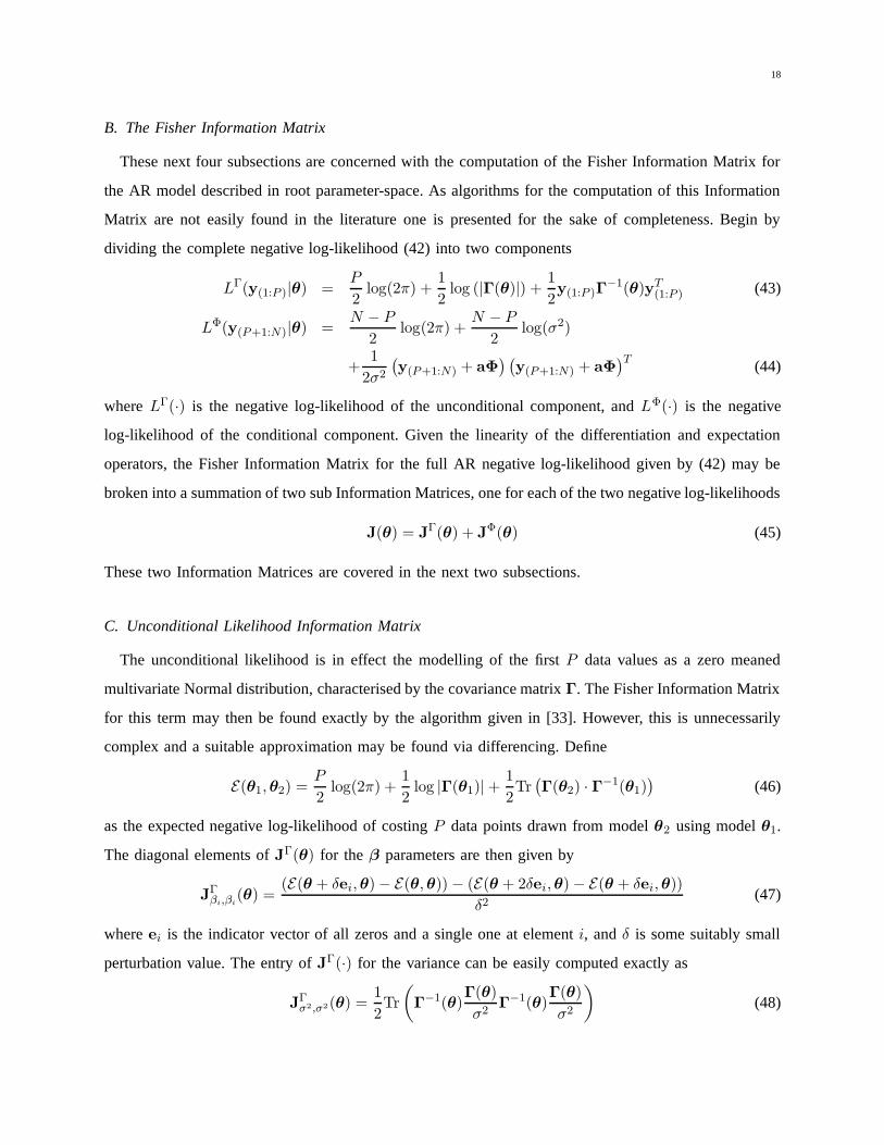
B. The Fisher Information Matrix
These next four subsections are concerned with the computation of the Fisher Information Matrix for
the AR model described in root parameter-space. As algorithms for the computation of this Information
Matrix are not easily found in the literature one is presented for the sake of completeness. Begin by
dividing the complete negative log-likelihood (42) into two components
LΓ(y(1:P )|θ) =P
2log(2π) +
1
2log (|Γ(θ)|) +
1
2y(1:P )Γ
−1(θ)yT(1:P ) (43)
LΦ(y(P+1:N)|θ) =N − P
2log(2π) +
N − P
2log(σ2)
+1
2σ2
(
y(P+1:N) + aΦ) (
y(P+1:N) + aΦ)T
(44)
where LΓ(·) is the negative log-likelihood of the unconditional component, and LΦ(·) is the negative
log-likelihood of the conditional component. Given the linearity of the differentiation and expectation
operators, the Fisher Information Matrix for the full AR negative log-likelihood given by (42) may be
broken into a summation of two sub Information Matrices, one for each of the two negative log-likelihoods
J(θ) = JΓ(θ) + JΦ(θ) (45)
These two Information Matrices are covered in the next two subsections.
C. Unconditional Likelihood Information Matrix
The unconditional likelihood is in effect the modelling of the first P data values as a zero meaned
multivariate Normal distribution, characterised by the covariance matrix Γ. The Fisher Information Matrix
for this term may then be found exactly by the algorithm given in [33]. However, this is unnecessarily
complex and a suitable approximation may be found via differencing. Define
E(θ1,θ2) =P
2log(2π) +
1
2log |Γ(θ1)|+
1
2Tr(
Γ(θ2) · Γ−1(θ1))
(46)
as the expected negative log-likelihood of costing P data points drawn from model θ2 using model θ1.
The diagonal elements of JΓ(θ) for the β parameters are then given by
JΓβi,βi
(θ) =(E(θ + δei,θ)− E(θ,θ)) − (E(θ + 2δei,θ)− E(θ + δei,θ))
δ2(47)
where ei is the indicator vector of all zeros and a single one at element i, and δ is some suitably small
perturbation value. The entry of JΓ(·) for the variance can be easily computed exactly as
JΓσ2,σ2(θ) =
1
2Tr
(
Γ−1(θ)Γ(θ)
σ2Γ−1(θ)
Γ(θ)
σ2
)
(48)

19
where Tr(·) denotes the trace operator. The previous work by Fitzgibbon [31] on AR models did not
compute the FIM for the unconditional component, instead approximating it by absorbing it into the FIM
for the conditional component. In the case of the AR model parametrised in root space however, it is
advantageous to do so, as the addition of the diagonalised JΓ(·) to JΦ(·) helps significantly to stabilise
the matrix, which may be ill conditioned if the model has two roots that almost coincide.
D. Conditional Likelihood Information Matrix
It now remains to compute JΦ(·) for the conditional component. Begin by defining the ‘error’ poly-
nomial as
en ≡ en(q) ≡ en(p,y, q) =P∏
i=1
(1− piq)yn (49)
where q is a formal polynomial variable. Now, consider the expression
N − P
2log(2π) +
N − P
2log(σ2) +
1
2σ2
N∑
n=P+1
en(p,y, q1)en(p,y, q2) (50)
Expanding the polynomials in the right hand term and then making the substitution qk1 = qk
2 = yn−k
yields the the conditional part of the negative log-likelihood as in (42). The second derivatives of (50)
with respect to the root parameters βi, βj are then found by expanding
∂2LΦ(y|θ)
∂βi∂βj
=1
σ2
N∑
n=P+1
(
∂2en(q1)
∂βi∂βj
en(q2) +∂en(q1)
∂βi
∂en(q2)
∂β2
)
(51)
and subsequently making the substitutions qk1 = qk
2 = yn−k. The Fisher Information Matrix is then found
by taking expectation with respect to the data. Recalling that en(·) = zn, the first term in (51) vanishes
under expectations and we are left with
JΦ(βi,βj)
(θ) =N − P
σ2Ey
[
∂en(q1)
∂βi
∂en(q2)
∂β2
]
(52)
The expectation of (52) is simply found by further substituting
ynyn−k = γk (53)
where γk is the theoretical k-th autocovariance of the sequence, i.e. γk = Ey [ynyn−k] = Ey [yn−kyn]
[1]. The FIM also contains entries for the variance parameter σ2. The FIM entry for the (βi, σ2) and
(σ2, σ2) terms are given by
JΦ(βi,σ2)(θ) = − 1
2σ2
N∑
n=P+1
Ey
[
vn∂zn∂βi
]
= 0 (54)
JΦ(σ2 ,σ2)(θ) =
1
(σ2)3
N∑
n=P+1
Ey
[
z2n
]
− N − P
2(σ2)2=N − P
2(σ2)2(55)

20
The expectation in (55) is obviously the innovation variance. The expectation in (54) is zero because
the derivative of zn with respect to any βi will necessarily remove the yn term; as all observations yi
that arrived before time n cannot depend on vn, the cross-covariance between these terms must be zero.
The next section presents an algorithm for computing the derivatives of en(q) with respect to the root
parameters, so as to allow computation of (51).
E. Fisher Information Matrix Algorithm
Before we can compute the FIM, we must have a way of expanding polynomial expressions of the
form p(q1) · p(q2) and collect the resulting terms. Assume we have two polynomials in terms of two
variables q1 and q2, with coefficients c and d, respectively. We wish to find the resulting coefficients of
the bivariate polynomial g after the two univariate polynomials are multiplied together, i.e.
g(q1, q2) = c(q1) · d(q2) (56)
These terms can be easily computed by taking the outer product cT d of the two coefficient vectors. The
contents of the resulting matrix map to
cTd =
c1d1 c1d2 c1d3 ... c1dP
c2d1 c2d2...
c3d1. . . cP−2dP
... cP−1dP−1 cP−1dP
cPd1 ... cPdP−2 cP dP−1 cPdP
(57)
If our polynomials represent the A(D) polynomial of an autoregressive model, and we seek the expectation
of two finite length delayed and scaled sub-sequences of y, we need collect the terms based on the relative
differences in powers of their polynomial variables. As c1 and d1 are the q terms, c2 and d2 the q2 terms,
etc., we quickly see that all the qk1q
k2 terms lie on the main diagonal, the qk
1qk−12 , qk
1qk+12 terms lie on the
first off diagonal, and so on. It follows that the structure of the matrix in terms of differences between
degree of polynomial variables is a Toeplitz matrix given by toep([0, ..., P − 1]). Thus to collect all the
qk1q
k2 terms we can merely sum the main diagonal; to collect the qk
1qk−12 , qk
1qk+12 terms we sum the first
off diagonals, and so on. We define the vector valued function M(·) which takes two polynomial vectors
and returns the sums of terms of the same relative degree. The sum of terms of relative degree i are
given by
M|i|(c,d) = Tr(
(cT d) · toep(ei))
(58)

21
where ei is the indicator vector of all zeros and a single one at element i and Tr(·) indicates the trace
operator. We now must find a way of easily computing the derivatives of polynomial coefficients with
respect to their root-parameters. We assume we have a vector of poles p of the error polynomial e(q).
We assume these roots are sorted thus
p = [α1, ..., αPR, r1e
jω1 , r1e−jω1 , ..., rPC
ejωPC , rPCe−jωPC ] (59)
β = [α1, ..., αPR, r1, w1, ..., rPC
, wPC] (60)
where β is a sorted vector of root-space parameters. The derivatives of coefficients of e(q) with respect
to elements of β are easily found by exploiting the fact that the polynomial is already factored into a
series of roots which contain at most two root-space parameters. We define the function d(·) which takes
a list of roots and produces the derivatives of the resulting polynomial coefficients with respect to a β
parameter. First derivatives, i.e. with respect to βi are given by
d(p, βi) = κ(βi) · poly(p′(βi)) (61)
Table II gives values for κ(·) and p′(·), where u and v represent the indices of the two complex poles
containing parameters ri and ωi. The \ operator is used to indicate that an element of a vector should be
removed, i.e. (a \ i) removes the i-th element from vector a. Given these definitions, and recalling (51),
entry (βi, βj) of the Fisher Information Matrix is found as
Ey
[
∂2L(y|θ)
∂βi∂βj
]
=N − P
σ2M(d(p, βi),d(p, βj)) · [γ0, ..., γP−1]
T (62)
where γk is the k-th theoretical autocovariance of the sequence y and p is the vector of roots of the
error polynomial en(q) given in (49).
F. Parameter Estimation
The issue of estimation of model parameters β, σ2 from a measurement sequence y is considered in
this subsection. Closed form solutions for the MML estimator of β are difficult to obtain, so a numerical
search is employed. The estimates for σ2, assuming a scale invariant prior, can be found explicitly, so at
each evaluation of the cost function a suitable σ2 is estimated, given an estimate of β.
1) Maximum Likelihood Estimate of σ2: The Maximum Likelihood estimator for σ2 is derived first.
Begin by noting that σ2 can be factorised out of the autocovariance matrix Γ(θ) in (42), and the negative
log-likelihood may be rewritten as
L(y|θ) =N
2log(2π) +
1
2log(
(
σ2)P · |Γ∗(θ)|
)
+1
2σ2y(1:P )Γ
∗−1(θ)yT(1:P )
+N − P
2log(σ2) +
1
2σ2
(
y(P+1:N) + aΦ) (
y(P+1:N) + aΦ)T −N log ε (63)
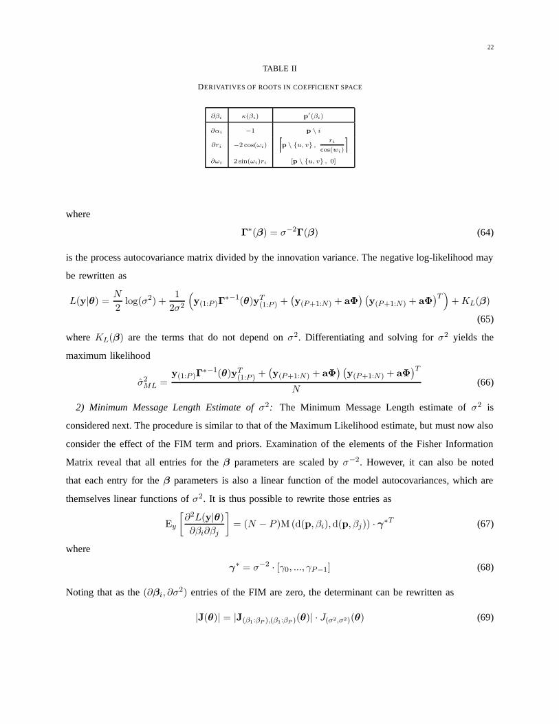
22
TABLE II
DERIVATIVES OF ROOTS IN COEFFICIENT SPACE
∂βi κ(βi) p′(βi)
∂αi −1 p \ i
∂ri −2 cos(ωi)
p \ u, v ,
ri
cos(wi) ∂ωi 2 sin(ωi)ri [p \ u, v , 0]
where
Γ∗(β) = σ−2Γ(β) (64)
is the process autocovariance matrix divided by the innovation variance. The negative log-likelihood may
be rewritten as
L(y|θ) =N
2log(σ2) +
1
2σ2
(
y(1:P )Γ∗−1(θ)yT
(1:P ) +(
y(P+1:N) + aΦ) (
y(P+1:N) + aΦ)T)
+KL(β)
(65)
where KL(β) are the terms that do not depend on σ2. Differentiating and solving for σ2 yields the
maximum likelihood
σ2ML =
y(1:P )Γ∗−1(θ)yT
(1:P ) +(
y(P+1:N) + aΦ) (
y(P+1:N) + aΦ)T
N(66)
2) Minimum Message Length Estimate of σ2: The Minimum Message Length estimate of σ2 is
considered next. The procedure is similar to that of the Maximum Likelihood estimate, but must now also
consider the effect of the FIM term and priors. Examination of the elements of the Fisher Information
Matrix reveal that all entries for the β parameters are scaled by σ−2. However, it can also be noted
that each entry for the β parameters is also a linear function of the model autocovariances, which are
themselves linear functions of σ2. It is thus possible to rewrite those entries as
Ey
[
∂2L(y|θ)
∂βi∂βj
]
= (N − P )M (d(p, βi),d(p, βj)) · γ∗T (67)
where
γ∗ = σ−2 · [γ0, ..., γP−1] (68)
Noting that as the (∂βi, ∂σ2) entries of the FIM are zero, the determinant can be rewritten as
|J(θ)| = |J(β1:βP ),(β1:βP )(θ)| · J(σ2 ,σ2)(θ) (69)

23
The message length may then be rewritten as
I(y,θ) = L(y|θ) − log h(σ2) +1
2log J(σ2 ,σ2)(θ) +KI(β) (70)
= L(y|θ) + log(σ2)− log(σ2) +KI(β) (71)
where KI(β) are all the terms not dependent on σ2. Clearly the effect of the Fisher and the prior terms
cancel, and render the MML estimate for σ2 to be
σ2MML = σ2
ML (72)
where σ2ML is given by (66).
3) Minimum Message Length Estimate of β: To find the estimates for β a numerical search is
employed; this can be prone to some instabilities due to the FIM becoming near singular for certain
parameter combinations, so a diagonal search stabilisation is applied. The procedure for finding the
MML estimates for an AR(P) model is then given by
1) Find initial coefficient estimates, a0, for an AR(P) model using a suitable estimation scheme; the
Burg method is recommended as it is quick and provides quite good estimates.
2) Extract the root structure, β0, of our initial estimates a0.
3) Numerically search for the MML estimates, βMML, within this given root structure, using the
diagonal search modification of the conditional FIM matrix, with the estimates β0 as a starting
point. The diagonal search modification is a simple robust approximation of the coding quantum,
and is given by1
2log |JΦ(θ)| ≈ 1
2
P+1∑
i=1
log(
JΦi,i(θ) + 1
)
(73)
A search performed under this regime will minimise the trade-off between the coding volume and
the negative log-likelihood, under the assumption that the parameters are uncorrelated. While this
is a false assumption in the case of AR models, and may lead to estimates that yield slightly longer
message lengths than if the full FIM was used, the fact that the diagonal elements of the FIM
generally dominate the off-diagonals, and the increased robustness in the search makes it a useful
approximation.
4) Once the search is complete, the Message Length I(y, θMML) of the estimated model is computed
by partially decorrelating parameters in the FIM, if required.
It also becomes clear at this point that parameterisation of the AR model in terms of root-parameters has
another advantage: for a given structure, the stationarity constraints reduce to a search within a hypercube,

24
with parameters bounded according to their type, i.e. αi ∈ (−1, 1), ri ∈ (0, 1) and ωi ∈ (0, π). This is
in contrast to a search in a-space where the stationarity region is bounded by a much more complex
polytope.
4) Derivatives of the Message Length: To improve the convergence of the search, the derivatives of
the message length can be computed. Begin with the derivatives of the negative log-likelihood w.r.t. to
βi
∂L(y|θ)
∂βi
=1
2Tr
(
Γ−1(θ)) · ∂Γ(θ))
∂βi
)
− 1
2y(1:P )Γ
−1(θ)∂Γ(θ)
∂βi
Γ−1(θ)yT(1:P ) (74)
+1
σ2
N∑
n=P+1
zn(β,y)∂zn(β,y)
∂βi(75)
where
zn(β,y) = yn +P∑
k=1
ak(β) · yn−k (76)
The derivatives of the coefficients a w.r.t. to root parameters can be computed as per the elements of the
Fisher Information matrix. Next the prior terms must be differentiated:
∂ log hr(αi)
∂αi=
α
1− α2(77)
∂ log hu(αi)
∂αi= 0 (78)
∂ log h(ri, ωj)
∂ωj=
cosωi
sinωi(79)
Finally, the Fisher Information terms must be differentiated. Under the diagonal approximation this
reduces to∂F (θ)
∂βi=
1
2
P∑
j=1
∂Jj,j(θ)
∂βi
(
JΦj,j(θ) + 1
)−1(80)
where∂Jj,j(θ)
∂βi
=P∑
k=1
∂
∂βi
Mk(d(p, βj),d(p, βj)) ·γk−1
σ2
(81)
The complete derivatives of the message length are then
∂I(y,θ)
∂βi=∂L(y|θ)
∂βi+∂F (θ)
∂βi− ∂ log h(θ)
∂βi(82)
Work by Karanosos [34] has given expressions for the model autocovariances with respect to the model
poles, and this can be used as a basis for finding the required derivatives.
25
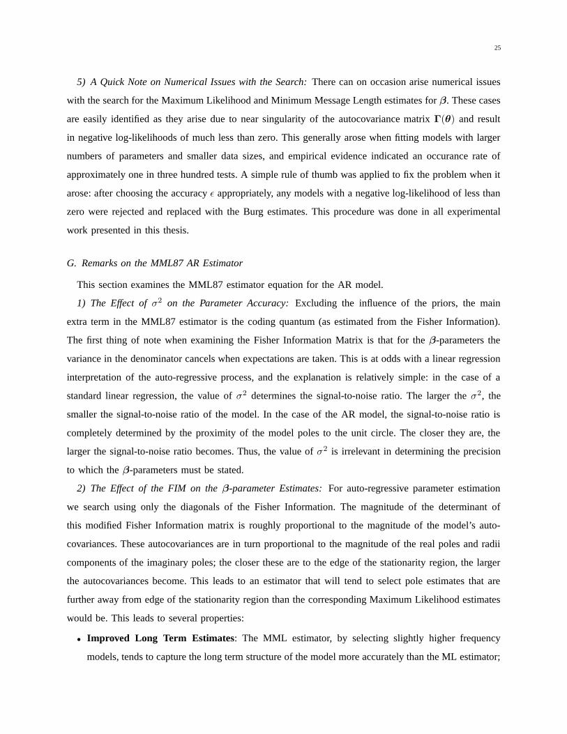
5) A Quick Note on Numerical Issues with the Search: There can on occasion arise numerical issues
with the search for the Maximum Likelihood and Minimum Message Length estimates for β. These cases
are easily identified as they arise due to near singularity of the autocovariance matrix Γ(θ) and result
in negative log-likelihoods of much less than zero. This generally arose when fitting models with larger
numbers of parameters and smaller data sizes, and empirical evidence indicated an occurance rate of
approximately one in three hundred tests. A simple rule of thumb was applied to fix the problem when it
arose: after choosing the accuracy ε appropriately, any models with a negative log-likelihood of less than
zero were rejected and replaced with the Burg estimates. This procedure was done in all experimental
work presented in this thesis.
G. Remarks on the MML87 AR Estimator
This section examines the MML87 estimator equation for the AR model.
1) The Effect of σ2 on the Parameter Accuracy: Excluding the influence of the priors, the main
extra term in the MML87 estimator is the coding quantum (as estimated from the Fisher Information).
The first thing of note when examining the Fisher Information Matrix is that for the β-parameters the
variance in the denominator cancels when expectations are taken. This is at odds with a linear regression
interpretation of the auto-regressive process, and the explanation is relatively simple: in the case of a
standard linear regression, the value of σ2 determines the signal-to-noise ratio. The larger the σ2, the
smaller the signal-to-noise ratio of the model. In the case of the AR model, the signal-to-noise ratio is
completely determined by the proximity of the model poles to the unit circle. The closer they are, the
larger the signal-to-noise ratio becomes. Thus, the value of σ2 is irrelevant in determining the precision
to which the β-parameters must be stated.
2) The Effect of the FIM on the β-parameter Estimates: For auto-regressive parameter estimation
we search using only the diagonals of the Fisher Information. The magnitude of the determinant of
this modified Fisher Information matrix is roughly proportional to the magnitude of the model’s auto-
covariances. These autocovariances are in turn proportional to the magnitude of the real poles and radii
components of the imaginary poles; the closer these are to the edge of the stationarity region, the larger
the autocovariances become. This leads to an estimator that will tend to select pole estimates that are
further away from edge of the stationarity region than the corresponding Maximum Likelihood estimates
would be. This leads to several properties:
• Improved Long Term Estimates: The MML estimator, by selecting slightly higher frequency
models, tends to capture the long term structure of the model more accurately than the ML estimator;

26
as has been mentioned previously, given the nonlinear relationship between model pole magnitudes
and resulting time constants, a slight underestimation in pole magnitude will lead to lower long term
errors than a slight overestimation of model pole positions.
• Larger Scale Estimates: The Maximum Likelihood estimator selects the coefficient estimates that
minimise the resulting residual variance. The MML87 estimates will necessarily differ from the ML
estimates (due to the influence of the Fisher Information term), and thus must result in slightly
inflated residual variance.
The improved long term estimation of the MML87 estimator is tested extensively by Monte Carlo
experiments in the results section of this tech report, and the experimental evidence suggests the MML87
estimates better capture the long-term behaviour of the underlying process.
3) The AR(1) Estimator of αMML for the Reference Prior: Estimation of the α parameter for AR(1)
models using the Reference prior throws up an interesting point. In this case the Reference prior is also
a Jeffrey’s prior, and when the MML87 approximation is used with a Jeffrey’s prior the effect of the
Fisher Information Matrix on the parameter estimates is exactly cancelled by the effect of the prior [2];
the estimates then coincide with the Maximum Likelihood estimates. However, when the effect of the
curvature of the prior is taken into consideration the addition of the correction term means the effects of
the prior and Fisher do not cancel. Experimental results demonstrate that MML87 estimator for AR(1)
parameters outperforms the Maximum Likelihood estimator even when using the Reference prior.
V. MOVING AVERAGE (MA) MODELS
The next second class of model examined in this technical report is the Moving Average (MA) model.
An MA model can be formed from the ARMA model by setting P = 0. The MA explanation of
measurement yn is then given by
yn =
P∑
i=1
civn−i + vn (83)
where vn is a random disturbance, again assumed to be i.i.d. as vn ∼ N (0, σ2). Order selection of MA
processes using MML has been studied previously by Sak et al [32]; however, in that case the inferences
were based on the conditional likelihood. In contrast, the work presented here is based on the exact
unconditional likelihood of the data y, and has also been extended to estimation of the c parameters.
The total prior probability density over the MA model is reduced to
h(θ) = h(Q) · h(c) · h(σ2) (84)
where the priors are chosen as per Section (III).
27
−1 −0.5 0 0.5 10
2
4
6
8
10
12
14
c
log−
dete
rmin
ant
Exact FIMAsymptotic FIM
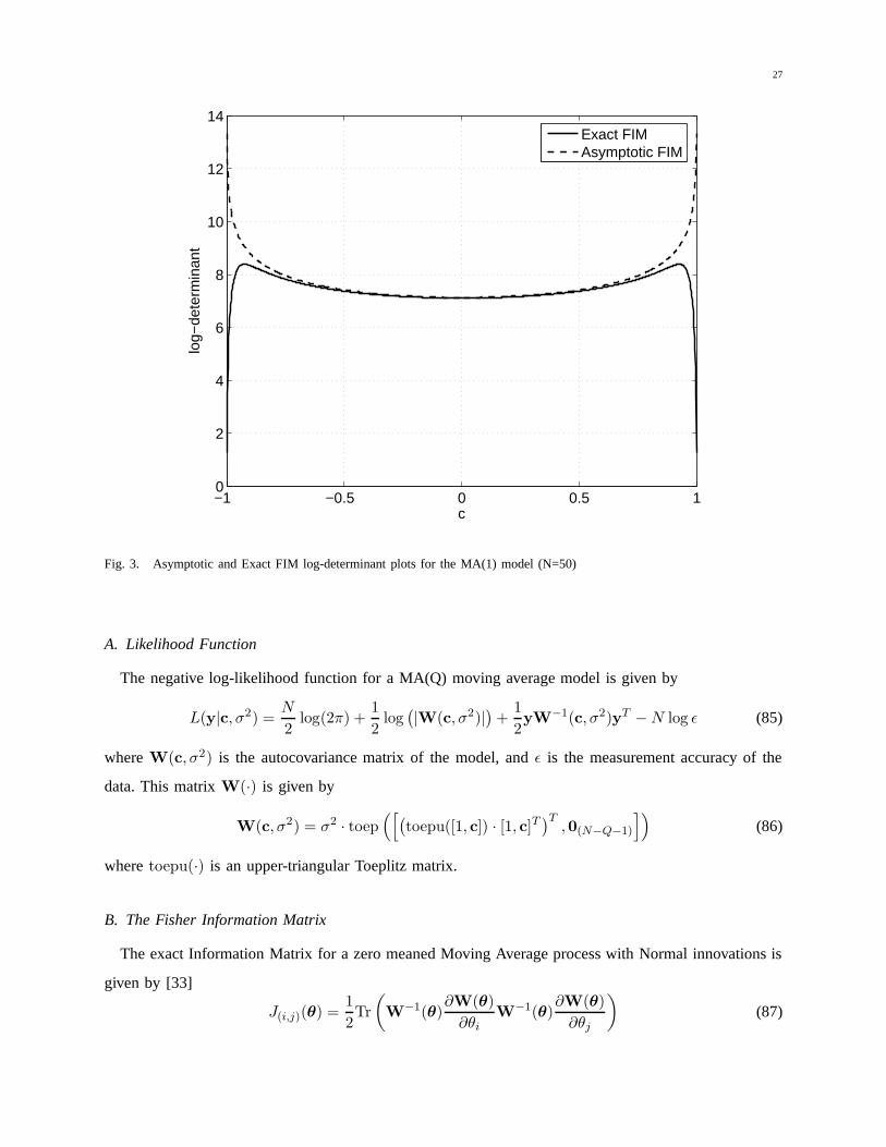
Fig. 3. Asymptotic and Exact FIM log-determinant plots for the MA(1) model (N=50)
A. Likelihood Function
The negative log-likelihood function for a MA(Q) moving average model is given by
L(y|c, σ2) =N
2log(2π) +
1
2log(
|W(c, σ2)|)
+1
2yW−1(c, σ2)yT −N log ε (85)
where W(c, σ2) is the autocovariance matrix of the model, and ε is the measurement accuracy of the
data. This matrix W(·) is given by
W(c, σ2) = σ2 · toep([
(
toepu([1, c]) · [1, c]T)T,0(N−Q−1)
])
(86)
where toepu(·) is an upper-triangular Toeplitz matrix.
B. The Fisher Information Matrix
The exact Information Matrix for a zero meaned Moving Average process with Normal innovations is
given by [33]
J(i,j)(θ) =1
2Tr
(
W−1(θ)∂W(θ)
∂θi
W−1(θ)∂W(θ)
∂θj
)
(87)

28
In particular, it is important to note that the entries are not merely functions of the parameters scaled
by the number of data points; this is due to the fact that the data y is not i.i.d. The largest issue of
concern surrounding the use of the exact Information Matrix in an MML87 formulation of the Moving
Average problem is its instability. There are many combinations of parameters that yield near singular
Information Matrices, and this is clearly are a source of great concern for an MML87 application. In this
work the asymptotic Information Matrix is used in place of the exact Matrix. Although for small amounts
of data the exact and the asymptotic Information Matrices will differ considerably as the zeroes of the
c parameters approach the boundary of the unit circle, the increased stability of the asymptotic variant
is deemed to outweigh any discrepancies in those regions where the exact matrix is also stable. Figure
3 shows a plot of the log-determinant of the exact FIM vs the log-determinant of the asymptotic FIM
for the MA(1) model for N = 50. The two coincide closely near c = 0, and begin to diverge as c→ 1.
As N increases, the curves will coincide for an increasingly larger region around c = 0, and eventually
converge as N → ∞, as is to be expected. Using Whittle’s asymptotic Fisher Information Matrix [35],
entry (θi, θj) is approximated by
J(θi,θj)(θ) ≈ N
4π
∫ π
−π
∂φ(ω)
∂θi· ∂φ(ω)
∂θj
φ2(ω)dω (88)
where N is the size of the dataset, and φ(ω) is the spectral power density function given by
φ(ω) = γ0 + 2∞∑
k=1
γk cos(kω) (89)
For ARMA processes the integrals in (88) can be solved exactly to yield simple expressions for the
Information Matrix [1]. In the case of the Moving Average process, the asymptotic Information Matrix
is given by
J(θ) = N
Ew
[
wT(1:Q)w(1:Q)
]
σ20
01
2 (σ2)2
(90)
where w = [w1, ..., wQ] is a sequence assumed to be generated from an auxilliary AR(Q) model thus
wn +
Q∑
i=1
ciwn−i = vn (91)
and
Ew
[
wT(1:Q)w(1:Q)
]
= Γw(θ) = toep([
γw0 , . . . , γ
wQ−1
])
(92)

29
is the Q × Q theoretical autocovariance matrix generated from the auxilliary AR(Q) process given by
(91), i.e. γwk = Ew [wnwn−k] = Ew [wn−kwn].
C. Parameter Estimation
This section examines the issue of estimating the c and σ2 parameters for the moving average model.
1) Maximum Likelihood Estimation of the Noise Variance: It is possible to find closed form maximum
likelihood estimates for the innovation variance; begin by factorising the noise variance σ2 out of the
negative log-likelihood function
L(y|c, σ2) =N
2log(2π) +
1
2log(
(
σ2)N · |W∗(c)|
)
+1
2σ2yW∗−1(c)yT (93)
where
W∗(c) =1
σ2W(c, σ2) (94)
is the process autocovariance matrix divided by the innovation variance. The negative log-likelihood may
be rewritten as
L(y|θ) =N
2log(σ2) +
1
2σ2yW∗−1(c)yT +KL(c) (95)
where KL(c) are those terms not dependent on σ2. Differentiating with respect to to σ2, and solving
yields
σ2ML =
yW∗−1(c)yT
N(96)
2) Minimum Message Length Estimation of the Noise Variance: Given the chosen priors, it is also
possible to find a closed form MML estimator for the innovation variance. Examination of the asymptotic
Fisher Information Matrix given by (90) reveals that it depends on the autocovariance matrix of the
auxilliary AR process. This autocovariances contain σ2 as a factor, and thus the determinant of the FIM
may be expressed as
|J(θ)| = |Γ∗w(θ)| · N
(Q+1)
2σ2(97)
where
Γ∗w(θ) = σ−2Γw(θ) (98)
is the auxilliary process autocovariance matrix divided by the innovation variance. The message length
may then be rewritten as
I(y,θ) =N
2log(σ2) +
1
2σ2yW∗−1(c)yT + log(σ2)− 1
2log(σ4) +KI(c) (99)

30
where KI(c) are those terms of the message length not dependent on σ2. The extra terms due to the
prior and Fisher cancel, and upon simplification the MML estimator for the variance is also given by
σ2MML =
yW∗−1(c)yT
N= σ2
ML (100)
3) Minimum Message Length Estimation of c: The derivatives of the negative log-likelihood w.r.t. c
are given by
∂L
∂ci=
1
2Tr
(
W−1(
c, σ2) ∂W
(
c, σ2)
∂ci
)
− 1
2yW−1
(
c, σ2) ∂W
(
c, σ2)
∂ciW−1
(
c, σ2)
yT (101)
The derivatives of the message length w.r.t. c are given by
∂I(y,θ)
∂ci=∂L
∂ci+
1
2Tr
(
J−1(θ)∂J(θ)
∂ci
)
(102)
where derivatives of the autocovariances can be computed as per [33].
4) The CLMML Estimator: This section presents an alternate parameter estimator for Moving Average
models that is based on a Conditional Likelihood scheme [1]. In this scheme, for Moving Average models,
the innovations are estimated by inversion of the moving average model, and the set of coefficients that
minimise the variance of innovations is sought as the estimate. The CLMML works in a similar fashion,
but instead uses the innovations to estimate the negative log-likelihood, and subsequently estimate the
message length of the model. The first step is to estimate the innovations, v, via the autoregressive
process
vn = yn −Q∑
i=1
civn−i (103)
with initial conditions
v(1−Q):0 = 0 (104)
Once the innovations have been estimated, the next step is to approximate the Message Length of the
exact model as
I(y, c, σ2) ≈ N
2
(
log (2π) + log(
σ2)
+ 1)
+1
2log |J
(
c, σ2)
| − log h(
c, σ2)
+ κM (Q+ 1) (105)
where κM (·) is MML87 dimensionality constant, and
σ2 =vT v
N(106)
is the estimate of the innovation variance. The CLMML estimates are then those c, σ2 that minimise (105)
with v estimated via (103). These estimates were found using the gradient free multi-level coordinate
search [36]. To ensure estimates were invertible, the search was conducted in the partial autocorrelation
31
space. In this space, the admissible values that characterise an invertible moving average process are
constrained to lie within a Q-dimensional hypercube bounded on (−1, 1) in all dimensions. A one-to-one
transformation exists between partial autocorrelation space and coefficient space [37], [38], and this was
applied to find the message length approximation.
D. Remarks on the MML87 MA Estimator
The MML87 estimator for the Moving Average model behaves in a similar fashion to the MML
estimator for the AR models. Given uniform priors on c and the scale invariant prior on σ2, the only
term that differs between the ML and the MML estimator is the log-determinant of the FIM. This also
behaves in a similar fashion to the FIM for the autoregressive process. As the c parameters move closer
to the invertibility boundary, the log-determinant of the FIM becomes larger. This leads to two immediate
features of the MML87 Moving Average parameter estimator as compared to the Maximum Likelihood
estimator:
• Flatter Frequency Responses: The depth and steepness of troughs (such as bandstop, low-pass and
high-pass modes) in the frequency response of Moving Average model increases as its zeros approach
the boundary of the invertibility region. As the log-determinant of the FIM in the MML87 estimator
will drive the zeros further away from the boundary than the Maximum Likelihood estimator,
the frequency responses of the MML models will tend to be ‘flatter’ and more smeared. As a
consequence, these models will be less definite on how strongly the frequencies are being affected
by the model.
• Larger Scale Estimates: In a similar fashion to the MML AR model, the scale estimates of the
MML MA estimator will be larger than the corresponding ML estimates. This follows from the
observation that the ML estimator will select the estimates cML that minimise σ2ML. As cMML
must necessarily differ from cML, and as σ2MML is chosen in the same fashion as σ2
ML, it follows
that σ2MML > σ2
ML (except in the degenerate case where all the coefficients are zero).
These comments apply equally to the CLMML estimator when compared to a scheme based on simply
minimising the conditional negative log-likehood function.

32
VI. EXPERIMENTAL RESULTS
The following section details results of order selection and parameter estimation experiments performed
on AR and models. The MML87 criterion parameter estimation results are compared to Maximum
Likelihood (ML) and other commonly used parameter estimation schemes, and model selection results are
compared against the AIC, AICc, BIC, KICc and NML selection criteria. The results are presented in terms
of appropriate metrics for each experiment and model class, and suitably demonstrate the effectiveness
of the MML87 estimator at capturing the time behaviour of the models in question.
Subsection (VI-A) covers the procedures used to perform the experiments, Subsection (VI-B) briefly
summarises the competing selection criteria, and Subsection (VI-C) details the performance metrics used
to evaluate the resulting inferred models. Subsections (VI-D) and (VI-E) present and analyse the results
of the Monte-Carlo experiments for the AR and MA models, respectively.
A. Experimental Design
There were two types of experiments performed: parameter estimation and model selection. These are
detailed presently.
1) Parameter Estimation Experiments: Parameter estimation experiments are performed to evaluate
the performance of the MML87 criterion at estimating model parameters from data for a given model
structure. The process that was used is summarised as follows: for a particular model structure S, a set
of I ‘true’ models are randomly sampled from the prior distributions. A sequence of N data points is
then generated from each model, and from this data the parameter estimates are made by each of the
F competing parameter estimation schemes, using the known true structure S. Once all estimates have
been made, the test scores for each of the inferred models are calculated.
2) Order Selection Experiments: Order selection experiments are performed to evaluate the per-
formance of the MML87 criterion at selecting the ‘best’ model from amongst a group of competing
candidates. To this end, a set of I ‘true’ models was generated by sampling from the prior distributions,
and a sequence of N data was generated from each model. Models are then inferred for a range of
structures, S1, . . . , SK , starting from the ‘simplest’ (in terms of number of parameters) to the most
complex. The F various competing criteria are then required to select which model they prefer from the
candidate set, and test scores are generated for each selected model.
3) Experiments on Real Data: To perform tests on sets of real (i.e. non synthetic) data the following
procedure was used: the data was divided into windows of length N , each Ng samples apart. From this
all models from orders [1, P ] were estimated, and the various model selection criteria were used to select

33
from this set. The performance of each criterion was assessed by then finding negative log-likelihood,
multi-step SPE, single step SPE and single step log-likelihood scores over a window of Nf samples that
directly followed the window from which the models were drawn. The innovations used in computing
the multi-step SPE scores were estimated from the residuals of a Least Squares AR(20) fit to the data.
B. Alternative Criteria
There are many, many methods for model selection of time series models available in the literature:
necessarily we must restrict testing to a subset of all the available criteria, primarily due to time
restrictions. In particular we restrict our attention to the AIC, AICc, BIC, KICc and MDL criterion.
The first three are chosen due to their ‘classic’ status in the literature; AIC [9] was one of the very
earliest formal attempts at model selection, BIC [11] and MDL78 [14] are identical for linear models,
and AICc [10] was specifically introduced to compensate for the weaknesses of AIC. KICc [13] is a
relative newcomer and offers modern competition, and the NML criterion is the amongst the very latest
developments in model selection. For convenience, we summarise the formulas of the various criteria
below
AIC(k) = 2L(y|θML) + 2k (107)
AICc(k) = 2L(y|θML) + 2k +2k(k + 1)
N − k − 1(108)
BIC(k) = 2L(y|θML) + k logN (109)
KICc(k) = 2L(y|θML) +2(k + 1)N
N − k − 2−Nψ
(
N − k
2
)
+N logN
2(110)
where k is the total number of autoregressive and moving average parameters in the model, N is the
number of data samples, L(·) is the negative log-likelihood of the model, θML are the maximum-
likelihood estimates and ψ(·) is the digamma function. The latest MDL cost function for linear regression
[39] has been applied to auto-regressive model selection, and the NML ‘cost’ function for an AR model
is given by [40]
NML(y) =N − 2P
2log σ2
LS +P
2log
(
θLS
(
ΦΦT
N − P
)
θTLS
)
(111)
− log Γ
(
N − 2P
2
)
− log Γ
(
P
2
)
(112)
where θLS , σ2LS are the Least Squares estimates for model parameters and residual variance, and Γ(·) is
Riemann’s Gamma function.
34
C. Evaluation of Results
To compare the inferred models there must be suitable metrics upon which comparisons can be made.
There is no ‘single best’ metric to use, and each metric captures behaviour of a particular aspect of a
model’s performance. This section details the metrics that were chosen for evaluation. For the following
test metrics it is assumed that there is an inferred ARMA(P , Q) model with estimated parameters θ =[
a, c, σ2]
available. Although the metrics are presented for the full ARMA model structure, they may be
easily adapted for AR and MA models by ignoring the appropriate terms.
1) Squared Prediction Error: The Squared Prediction Error (SPE) criterion assesses the behaviour of
the coefficients of the model (i.e. a and c). There are two SPE criteria that can be used when assessing
ARMA family models: the one-step SPE, denoted SPE1, and the multi-step SPE, denoted SPENf, where
Nf is the number of forecast steps. Given an inferred time ARMA model ARMA(P , Q) and a time
series generated by the ‘true model’, y, with innovation sequence v, the one-step SPE for sample n is
defined as
SPE1(n) =
yn +
P∑
i=1
aiyn−i −Q∑
i=1
civn−i
2
(113)
and the total SPE1 over the whole sequence is given by
SPE1 =1
N −m
N∑
n=m
SPE1(n) (114)
The multi-step SPE is found by initialising the inferred model with values from the true sequences y
and v, and then forecasting over the next Nf samples by letting the model ‘run free’, driven by the
innovation sequence v. The SPENfscore is thus given by
yn = −P∑
i=1
aiyn−i +
Q∑
i=1
civn−i + vn
SPENf(n) =
1
Nf
Nf−1∑
i=0
(yn+i − yn+i)2 (115)
with initial conditions
y(n−P :n−1) = y(n−P :n−1) (116)
Finally, when comparing SPEs over many different models it is desirable to have them all on the same
footing in terms of the signal power. If this is not done, the error score for a model with low power output
may be swamped by the error score for a model with larger power output, even though in percentage
terms the error for the lower power model may be significantly greater. One method of normalisation

35
may be be easily performed by generating the true sequence y with an innovation sequence chosen to
render the γ0 of the process to be unity, i.e.
vn ∼ N(
0,σ2
γ0(θ)
)
(117)
where γ0(θ) is the zero-order autocovariance of the true generating process, and σ2 is the variance of
the ‘true’ innovation sequence. Obviously all these scores both require that the innovation sequence v
is available for observation. For synthetic tests where the true model is exactly known and the data
sequence y is generated from this model, this is clearly a reasonable assumption. For real data where
the innovation sequence is buried in the signal, it is possible to estimate it via an overparameterised
autoregressive process.
The one-step SPE measures the model’s ability to perform short term predictions and is akin to treating
the process as merely a linear regression on past measurements; it does not measure how well a model
has captured the longer term time behaviour of the sequence. The multi-step SPE on the other hand, puts
‘faith’ into the predictions made by the model and uses them to produce further predictions. The model
is no longer merely a linear regression; its ability to capture the behaviour of the model over time is
now under examination. Thus, while reasonable SPE1 scores are desirable, it is the SPENfscores of a
model that indicate how well it is modelling the long term structure of the data.
2) Negative Log-Likelihood and KL-Divergence: The negative log-likelihood criterion assesses all
parameters of the model at once. Basically, future unseen data is costed using the likelihood function
parameterised by the inferred model. Again, there are two variants: the one-step negative log-likelihood,
denoted L1, and the multiple-sample negative log-likelihood, denoted LNf, where Nf is the number of
samples to cost. The one-step likelihood can be easily computed from the one-step SPE as
L1(n) =1
2log (2π) +
1
2log σ2 +
SPE1(n)
2σ2(118)
and the L1 score for the entire sequence
L1 =1
N −m
N∑
n=m
L1(n) (119)
The multi-step negative-log-likelihood score is found instead by costing a length of the sequence as a
single multi-variate Gaussian distribution characterised by the autocovariances of the inferred model. This
captures long term structure of the coefficients as well as the effect of the scale parameter in one metric,
and is given by
LNf(n) =
Nf
2log (2π) +
1
2log |Γ(θ)|+ 1
2y(n:n+Nf−1)Γ
−1(θ)yT(n:n+Nf−1) (120)
36
where Γ(θ) is the (Nf ×Nf ) autocovariance matrix of the inferred ARMA model. If the true model is
known (i.e. tests are not being performed on real data), the multi-step Kullback-Leibler divergence can
be used instead. The KLNfscore is given by
KLNf=Nf
2log(2π) +
1
2log |Γ(θ)|+ 1
2Tr(
Γ(θ) · Γ−1(θ))
(121)
Although the multi-step negative log-likelihood/KL divergence scores evaluate all parameters of the
inferred model at once, they can be influenced heavily by the scale estimate. Poor estimation of the
coefficient parameters can result smaller increases in negative log-likelihood than can an under-estimation
of the scale parameter. If the innovation variance is considered a nuisance parameter, for instance in cases
where the main issue is to determine how much long term effect a shock to an AR model has on its
overall time response, the multi-step SPE score should be treated as a more revealing metric.
3) Order Selection: This criterion is often used to evaluate the performance of a model selection
criterion’s ability to correctly identify structure of the underlying model, i.e. to correctly estimate P
and Q. There are several arguments against the validity of this criterion as a gauge of an estimator’s
performance: first, due to the parameterisation of the model, or the mathematical form of the likelihood,
it is very possible that the estimates a, c and σ2 yield very high large negative log-likelihoods and
prediction errors when the correct model order is used, while a less complex model may yield much
better log likelihood/prediction errors. This is particular true when the amount of data from which the
inferences are drawn is very small in comparison to the number of parameters in the model. What then
is the point of knowing the true structure of the underlying model if the ability of this estimated model
to predict the behaviour of the true process is poor?
The second problem with this criterion is that it is only applicable in those cases where the structure of
the underlying model is both known, and known to be of the same class as the model being inferred from
the data. For real data, where the underlying generating model can never really be known, the concept
of correct order identification becomes somewhat meaningless.
D. Autoregressive Experiments
1) Parameter Estimation Experiments: The MML87 parameter estimator for the AR models was com-
pared against the Maximum Likelihood estimator, the Burg estimator [4], the Yule-Walker [1] estimator
and the Least Squares estimator. For each order it was tested for data sizes, N = k(3P + 1) where
k = 1, 2, 4. These data sizes were chosen to contain the minimum number of data points the Matlab
implementations required for the least squares estimates to be computed, and they represent a suitably
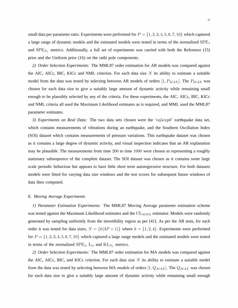
37
small data per parameter ratio. Experiments were performed for P = 1, 2, 3, 4, 5, 6, 7, 10 which captured
a large range of dynamic models and the estimated models were tested in terms of the normalised SPE1
and SPENfmetrics. Additionally, a full set of experiments was carried with both the Reference (15)
prior and the Uniform prior (16) on the radii pole components.
2) Order Selection Experiments: The MML87 order estimation for AR models was compared against
the AIC, AICc, BIC, KICc and NML criterion. For each data size N its ability to estimate a suitable
model from the data was tested by selecting between AR models of orders [1, PMAX ]. The PMAX was
chosen for each data size to give a suitably large amount of dynamic activity while remaining small
enough to be plausibly selected by any of the criteria. For these experiments, the AIC, AICc, BIC, KICc
and NML criteria all used the Maximum Likelihood estimates as is required, and MML used the MML87
parameter estimates.
3) Experiments on Real Data: The two data sets chosen were the ‘eq5exp6’ earthquake data set,
which contains measurements of vibrations during an earthquake, and the Southern Oscillation Index
(SOI) dataset which contains measurements of pressure variations. This earthquake dataset was chosen
as it contains a large degree of dynamic activity, and visual inspection indicates that an AR explanation
may be plausible. The measurements from time 200 to time 1000 were chosen as representing a roughly
stationary subsequence of the complete dataset. The SOI dataset was chosen as it contains some large
scale periodic behaviour but appears to have little short term autoregressive structure. For both datasets
models were fitted for varying data size windows and the test scores for subsequent future windows of
data then computed.
E. Moving Average Experiments
1) Parameter Estimation Experiments: The MML87 Moving Average parameter estimation scheme
was tested against the Maximum Likelihood estimates and the CLMML estimator. Models were randomly
generated by sampling uniformly from the invertibility region as per [41]. As per the AR tests, for each
order it was tested for data sizes, N = k(3P + 1) where k = 1, 2, 4. Experiments were performed
for P = 1, 2, 3, 4, 5, 6, 7, 10 which captured a large range models and the estimated models were tested
in terms of the normalised SPE1, L1, and KLNfmetrics.
2) Order Selection Experiments: The MML87 order estimation for MA models was compared against
the AIC, AICc, BIC, and KICc criterion. For each data size N its ability to estimate a suitable model
from the data was tested by selecting between MA models of orders [1, QMAX ]. The QMAX was chosen
for each data size to give a suitably large amount of dynamic activity while remaining small enough

38
to be plausibly selected by any of the criteria. For these experiments, the AIC, AICc, BIC, and KICc
criteria all used the Maximum Likelihood estimates as is required, and MML used the MML87 parameter
estimates.
VII. DISCUSSION OF RESULTS
A. Autoregressive Parameter Estimation Results
The Autoregressive parameter estimation test results are presented in Tables V and VI, with the
‘winning’ criterion highlighted in bold. These tables indicate that the MML87 parameter estimates are as
good as, and in most cases, superior to the ML, Burg and Yule-Walker estimates in terms of multi-step
SPE and single step SPE. The results are more pronounced for larger models being fitted to smaller
sequences of data. In terms of multi-step SPE, the MML estimator performs the best in all but case
(P = 2, N = 28, for the uniform prior), but in the loss is around 0.2% which is negligible. When the
MML87 estimator wins on SPE10 scores, it wins by up to as much as 50% (P = 10, N = 31, for the
uniform prior).
In terms of SPE1 results, MML does not always outperform the other estimators, and when it does it
is not by as large amounts as on multi-step SPE scores (as an example, for P = 10, N = 31, it wins
by approximately 20% on SPE1 scores). On the whole, however, the MML87 one step ahead prediction
errors are better than those achieved by the ML, Burg and Yule-Walker estimators, and in particular are
increasingly better as the number of datums per parameter grows smaller.
The way in which the MML87 estimator differs from the Maximum Likelihood, Burg, and to an extent,
Yule-Walker estimates can be revealed by examining a single experiment on an AR(10) process, drawn
from the larger experiment set. A sequence of 31 data points was generated from the 10-th order AR
process, At(q), given by
At(q) = 1 + 0.06465q−1 − 0.05855q−2 − 0.5921q−3 − 0.3985q−4
−0.0157q−5 + 0.07233q−6 + 0.05173q−7 − 0.01658q−8
+0.004312q−9 − 0.0004345q−10 (122)
This process was randomly generated by sampling from the prior, using uniform priors on the model
radii. The roots of At(q) are a mix of slow and fast real and complex poles. The Maximum Likelihood
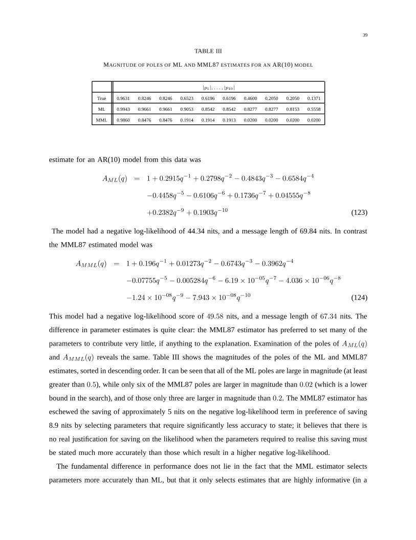
39
TABLE III
MAGNITUDE OF POLES OF ML AND MML87 ESTIMATES FOR AN AR(10) MODEL
|p1|, . . . , |p10|
True 0.9631 0.8246 0.8246 0.6523 0.6196 0.6196 0.4600 0.2050 0.2050 0.1371
ML 0.9943 0.9661 0.9661 0.9053 0.8542 0.8542 0.8277 0.8277 0.8153 0.5558
MML 0.9860 0.8476 0.8476 0.1914 0.1914 0.1913 0.0200 0.0200 0.0200 0.0200
estimate for an AR(10) model from this data was
AML(q) = 1 + 0.2915q−1 + 0.2798q−2 − 0.4843q−3 − 0.6584q−4
−0.4458q−5 − 0.6106q−6 + 0.1736q−7 + 0.04555q−8
+0.2382q−9 + 0.1903q−10 (123)
The model had a negative log-likelihood of 44.34 nits, and a message length of 69.84 nits. In contrast
the MML87 estimated model was
AMML(q) = 1 + 0.196q−1 + 0.01273q−2 − 0.6743q−3 − 0.3962q−4
−0.07755q−5 − 0.005284q−6 − 6.19 × 10−05q−7 − 4.036 × 10−06q−8
−1.24× 10−08q−9 − 7.943 × 10−08q−10 (124)
This model had a negative log-likelihood score of 49.58 nits, and a message length of 67.34 nits. The
difference in parameter estimates is quite clear: the MML87 estimator has preferred to set many of the
parameters to contribute very little, if anything to the explanation. Examination of the poles of AML(q)
and AMML(q) reveals the same. Table III shows the magnitudes of the poles of the ML and MML87
estimates, sorted in descending order. It can be seen that all of the ML poles are large in magnitude (at least
greater than 0.5), while only six of the MML87 poles are larger in magnitude than 0.02 (which is a lower
bound in the search), and of those only three are larger in magnitude than 0.2. The MML87 estimator has
eschewed the saving of approximately 5 nits on the negative log-likelihood term in preference of saving
8.9 nits by selecting parameters that require significantly less accuracy to state; it believes that there is
no real justification for saving on the likelihood when the parameters required to realise this saving must
be stated much more accurately than those which result in a higher negative log-likelihood.
The fundamental difference in performance does not lie in the fact that the MML estimator selects
parameters more accurately than ML, but that it only selects estimates that are highly informative (in a
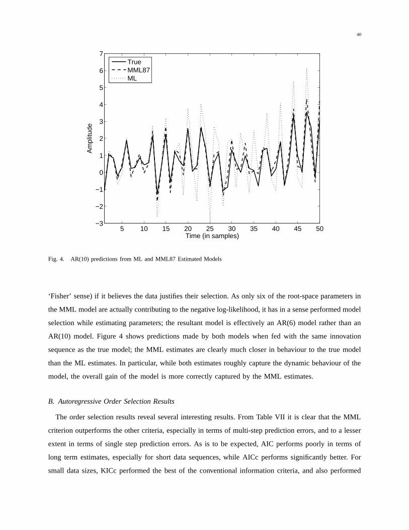
40
5 10 15 20 25 30 35 40 45 50−3
−2
−1
0
1
2
3
4
5
6
7
Time (in samples)
Am
plitu
de
TrueMML87ML
Fig. 4. AR(10) predictions from ML and MML87 Estimated Models
‘Fisher’ sense) if it believes the data justifies their selection. As only six of the root-space parameters in
the MML model are actually contributing to the negative log-likelihood, it has in a sense performed model
selection while estimating parameters; the resultant model is effectively an AR(6) model rather than an
AR(10) model. Figure 4 shows predictions made by both models when fed with the same innovation
sequence as the true model; the MML estimates are clearly much closer in behaviour to the true model
than the ML estimates. In particular, while both estimates roughly capture the dynamic behaviour of the
model, the overall gain of the model is more correctly captured by the MML estimates.
B. Autoregressive Order Selection Results
The order selection results reveal several interesting results. From Table VII it is clear that the MML
criterion outperforms the other criteria, especially in terms of multi-step prediction errors, and to a lesser
extent in terms of single step prediction errors. As is to be expected, AIC performs poorly in terms of
long term estimates, especially for short data sequences, while AICc performs significantly better. For
small data sizes, KICc performed the best of the conventional information criteria, and also performed
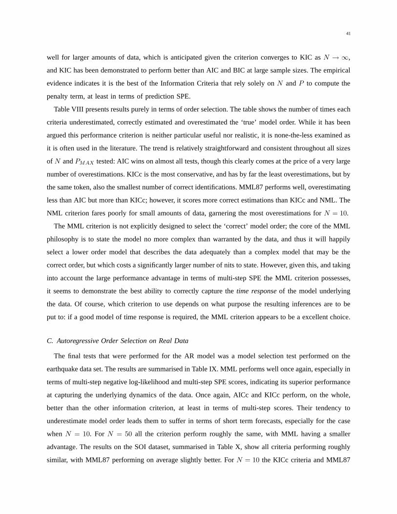
41
well for larger amounts of data, which is anticipated given the criterion converges to KIC as N → ∞,
and KIC has been demonstrated to perform better than AIC and BIC at large sample sizes. The empirical
evidence indicates it is the best of the Information Criteria that rely solely on N and P to compute the
penalty term, at least in terms of prediction SPE.
Table VIII presents results purely in terms of order selection. The table shows the number of times each
criteria underestimated, correctly estimated and overestimated the ‘true’ model order. While it has been
argued this performance criterion is neither particular useful nor realistic, it is none-the-less examined as
it is often used in the literature. The trend is relatively straightforward and consistent throughout all sizes
of N and PMAX tested: AIC wins on almost all tests, though this clearly comes at the price of a very large
number of overestimations. KICc is the most conservative, and has by far the least overestimations, but by
the same token, also the smallest number of correct identifications. MML87 performs well, overestimating
less than AIC but more than KICc; however, it scores more correct estimations than KICc and NML. The
NML criterion fares poorly for small amounts of data, garnering the most overestimations for N = 10.
The MML criterion is not explicitly designed to select the ‘correct’ model order; the core of the MML
philosophy is to state the model no more complex than warranted by the data, and thus it will happily
select a lower order model that describes the data adequately than a complex model that may be the
correct order, but which costs a significantly larger number of nits to state. However, given this, and taking
into account the large performance advantage in terms of multi-step SPE the MML criterion possesses,
it seems to demonstrate the best ability to correctly capture the time response of the model underlying
the data. Of course, which criterion to use depends on what purpose the resulting inferences are to be
put to: if a good model of time response is required, the MML criterion appears to be a excellent choice.
C. Autoregressive Order Selection on Real Data
The final tests that were performed for the AR model was a model selection test performed on the
earthquake data set. The results are summarised in Table IX. MML performs well once again, especially in
terms of multi-step negative log-likelihood and multi-step SPE scores, indicating its superior performance
at capturing the underlying dynamics of the data. Once again, AICc and KICc perform, on the whole,
better than the other information criterion, at least in terms of multi-step scores. Their tendency to
underestimate model order leads them to suffer in terms of short term forecasts, especially for the case
when N = 10. For N = 50 all the criterion perform roughly the same, with MML having a smaller
advantage. The results on the SOI dataset, summarised in Table X, show all criteria performing roughly
similar, with MML87 performing on average slightly better. For N = 10 the KICc criteria and MML87

42
0 0.1 0.2 0.3 0.4 0.510
−5
10−4
10−3
10−2
10−1
100
101
Frequency
Nor
mal
ised
Pow
er S
pect
ral D
ensi
ty
TrueMMLML
Fig. 5. Power Spectral Densities of MA(7) ML and MML estimates
show significantly better performance than the other criteria: both criteria tend to estimate lower model
orders on average, and in this case, with little structure present in the data, lower order models lead
to better fits. The NML criteria performs the worst on average, and tends to exhibit a large amount of
overfitting for N = 30.
D. Moving Average Parameter Estimation Results
The results for Moving Average Parameter estimation are presented in Table XI. The KL scores are
the average KL-divergences per datum over a forecast of 500 datapoints, i.e. the average KL500 scores
of all tests divided by 500. The general trend is reasonably straightforward: the MML87 estimates are
superior in terms of one step ahead SPE scores and KL-divergences in almost all cases; for the MA(1)
model with N = 4 the CLMML scheme achieves superior KL and SPE scores by a small margin. As
the number of data points increase for each order, the MML and ML estimates begin to perform very
similar, as would be expected. The good performance of the MML estimates is down, as is usually the
case, to the fact that when the ML estimates perform badly, they perform very badly. It is also interesting

43
TABLE IV
MAGNITUDE OF ZEROS OF ML AND MML87 ESTIMATES FOR AN MA(7) MODEL
|z1|, . . . , |z7|
True 0.9953 0.9953 0.9947 0.9947 0.8424 0.4417 0.2624
ML 0.9908 0.9785 0.9785 0.9775 0.9775 0.5755 0.5755
MML 0.9530 0.9548 0.9548 0.9372 0.9372 0.2931 0.2931
to note that the closest competitor to the full MML87 estimator is the CLMML estimator scheme, which
while in almost all cases is outperformed by the full MML estimator, comes quite close in terms of SPE
and KL-divergences.
The way in which the MML87 Moving Average parameter estimation scheme gains an advantage
over the Maximum Likelihood scheme (and those based on approximation of the likelihood) can be
demonstrated by examining a single test case. A sequence of 44 data points was drawn from the MA(7)
model
C(q) = 1 + 0.8674q−1 + 1.145q−2 − 0.4056q−3 − 0.5228q−4 (125)
−0.8172q−5 − 0.1137q−6 + 0.0957q−7 (126)
This model was generated by sampling uniformly from the invertibility region, and contains a mix of
real and complex zeros. The Maximum Likelihood estimate was given by
CML(q) = 1 + 0.908q−1 + 0.8979q−2 − 0.8093q−3 − 0.585q−4 (127)
−0.8963q−5 − 0.1258q−6 − 0.3003q−7 (128)
and the MML87 estimates are given by
CMML(q) = 1 + 0.7352q−1 + 0.8479q−2 − 0.6036q−3 − 0.5535q−4 (129)
−0.867q−5 − 0.1061q−6 − 0.06554q−7 (130)
The ML model achieved a training negative log-likelihood of 84.15 nits, with a message length of
103.06 nits. In contrast the MML model achieved a training negative log-likelihood of 84.5 nits, but a
message length of 100.31 nits. Thus it trades less than 0.4 nits of training score to reduce the message
length by almost 3 nits. The zeros of all three models are presented in Table IV. The most obvious thing to
note is that the zeros of the ML estimated model are much stronger in magnitude than the corresponding
zeros of the MML estimates; in particular, all the ML zeros are greater in magnitude than 0.5 while in

44
the case of the MML estimates two zeros are less than 0.3. The effect of this is shown quite clearly in
the Power Spectral Density plots of all three models, presented in Figure 5. Although the ML model
captures the depths of the troughs in the frequency response more accurately than the MML87 model,
the positions of the troughs are incorrect. This leads to a strong attenuation of the wrong frequencies,
which clearly has strong effects on the Kullback-Leibler divergence between the models. The MML87
estimator does not correctly capture the depths of the troughs, but more accurately estimates the position
of one of them (f ≈ 0.27) and by underestimating the strength of attenuation of the other bandstop
mode, causes the KL-divergence to be reduced. Again, the MML estimates refuse to ‘overcommit’ to a
more precise model, which is in this case one in which frequencies are more heavily attenuated, if it is
not warranted by the data.
E. Moving Average Order Selection Results
Finally, Tables XII and XIII summarise the Moving Average order selection results. In terms of KL-
divergences and SPE scores, MML87 is clearly superior for all data sizes and order ranges. KICc, BIC
and AICc all come in roughly second, with KICc performing better in general in terms of KL-divergences
and BIC performing better in several cases in terms of SPE scores. AIC performs roughly the worst in
terms of prediction scores, but an examination of Table XIII indicates that AIC wins in terms of number
of correct order identifications. The KICc criterion has the least amount of overfitting, but performs the
worst in terms of correct identifications, while MML87 performs roughly similar to BIC in terms of under
and over-estimation of model orders. BIC tends to overfit more than MML87 at smaller sample sizes,
but achieves more correct order identification results; this trend is slightly reversed as the number of data
points grow. The results seem to demonstrate that if good model selection in terms of KL divergence
and SPE1 scores are desired, then the MML87 criterion performs very well and is a suitable choice.
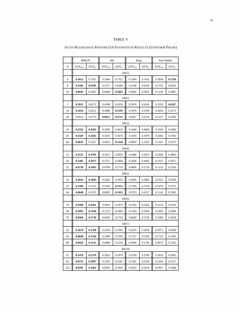
45
TABLE V
AUTO-REGRESSIVE PARAMETER ESTIMATION RESULTS (UNIFORM PRIOR)
MML87 ML Burg Yule-Walker
N SPE10 SPE1 SPE10 SPE1 SPE10 SPE1 SPE10 SPE1
AR(1)
4 0.2652 0.7261 0.3446 0.7527 0.3304 0.7435 0.2858 0.7256
8 0.1445 0.6185 0.1577 0.6200 0.1548 0.6193 0.1752 0.6263
16 0.0943 0.5847 0.0968 0.5845 0.0994 0.5852 0.1136 0.5887
AR(2)
7 0.2912 0.6172 0.4188 0.6326 0.3976 0.6242 0.3220 0.6107
14 0.1654 0.5211 0.1889 0.5195 0.1970 0.5199 0.2056 0.5273
28 0.0914 0.4773 0.0911 0.4731 0.0957 0.4739 0.1157 0.4786
AR(3)
10 0.2332 0.4302 0.3283 0.4624 0.3266 0.4600 0.3330 0.4584
20 0.1429 0.3645 0.1619 0.3676 0.1693 0.3679 0.2066 0.3766
40 0.0835 0.3327 0.0855 0.3318 0.0893 0.3321 0.1187 0.3375
AR(4)
13 0.2513 0.3703 0.3411 0.3933 0.3406 0.3875 0.3204 0.3803
26 0.1405 0.2977 0.1571 0.3004 0.1606 0.3002 0.1921 0.3071
52 0.0730 0.2695 0.0769 0.2710 0.0806 0.2710 0.1110 0.2760
AR(5)
16 0.2054 0.2693 0.2942 0.2932 0.3085 0.2883 0.3352 0.2959
32 0.1200 0.2152 0.1426 0.2151 0.1509 0.2159 0.1976 0.2273
64 0.0648 0.1915 0.0693 0.1913 0.0723 0.1917 0.1143 0.1983
AR(6)
19 0.1989 0.2401 0.2810 0.2470 0.2792 0.2426 0.3122 0.2559
38 0.1092 0.1958 0.1272 0.1960 0.1334 0.1964 0.1843 0.2068
76 0.0560 0.1739 0.0630 0.1754 0.0649 0.1756 0.1083 0.1818
AR(7)
22 0.1679 0.1768 0.2439 0.1942 0.2476 0.1926 0.2971 0.2040
44 0.0848 0.1356 0.1098 0.1393 0.1127 0.1393 0.1753 0.1504
88 0.0424 0.1221 0.0489 0.1234 0.0506 0.1236 0.0973 0.1295
AR(10)
31 0.1479 0.2379 0.2916 0.2879 0.2769 0.2789 0.2819 0.2682
62 0.0755 0.2097 0.1292 0.2241 0.1281 0.2230 0.1648 0.2257
124 0.0395 0.1963 0.0593 0.2020 0.0592 0.2019 0.0937 0.2048

46
TABLE VI
AUTO-REGRESSIVE PARAMETER ESTIMATION RESULTS (REFERENCE PRIOR)
MML87 ML Burg Yule-Walker
N SPE10 SPE1 SPE10 SPE1 SPE10 SPE1 SPE10 SPE1
AR(1)
4 0.2856 0.7263 0.3530 0.7430 0.3418 0.7339 0.2877 0.7206
8 0.1553 0.6183 0.1677 0.6198 0.1644 0.6187 0.1767 0.6244
16 0.0934 0.5793 0.0959 0.5794 0.0978 0.5799 0.1117 0.5837
AR(2)
7 0.2881 0.5039 0.3858 0.9397 0.3783 0.8832 0.3294 0.4372
14 0.1721 0.3537 0.1962 0.5010 0.1954 0.4924 0.2012 0.3206
28 0.0931 0.2020 0.0954 0.2473 0.0978 0.2811 0.1180 0.2330
AR(3)
10 0.2472 0.3920 0.3432 0.4366 0.3480 0.4295 0.3459 0.4304
20 0.1516 0.3375 0.1738 0.3456 0.1782 0.3452 0.2199 0.3542
40 0.0837 0.3023 0.0893 0.3044 0.0935 0.3048 0.1307 0.3103
AR(4)
13 0.2551 0.3461 0.3471 0.3842 0.3528 0.3794 0.3429 0.3754
26 0.1339 0.2775 0.1554 0.2830 0.1603 0.2822 0.2046 0.2924
52 0.0718 0.2540 0.0761 0.2548 0.0798 0.2549 0.1196 0.2604
AR(5)
16 0.2010 0.2577 0.2873 0.2849 0.2874 0.2794 0.3233 0.2856
32 0.1109 0.2098 0.1330 0.2164 0.1383 0.2164 0.1927 0.2249
64 0.0616 0.1907 0.0680 0.1924 0.0709 0.1926 0.1169 0.1989
AR(6)
19 0.1905 0.2189 0.2822 0.2404 0.2829 0.2384 0.3233 0.2479
38 0.1022 0.1752 0.1242 0.1807 0.1283 0.1809 0.1924 0.1903
76 0.0516 0.1613 0.0593 0.1631 0.0608 0.1633 0.1134 0.1690
AR(7)
22 0.1714 0.1618 0.2543 0.1823 0.2587 0.1804 0.3209 0.1951
44 0.0909 0.1334 0.1130 0.1382 0.1159 0.1386 0.1884 0.1477
88 0.0471 0.1197 0.0540 0.1206 0.0550 0.1206 0.1105 0.1259
AR(10)
31 0.1246 0.1063 0.1975 0.1207 0.1975 0.1179 0.2651 0.1360
62 0.0609 0.0893 0.0845 0.0934 0.0852 0.0933 0.1578 0.1048
124 0.0317 0.0830 0.0378 0.0842 0.0384 0.0842 0.0927 0.0907

47
TABLE VII
AR TEST SCORES ON SYNTHETIC DATA
Score MML87 AIC AICc BIC KICc NML
N = 10, P ∈ [1, 3]
SPE10 0.1857 0.3009 0.2566 0.2906 0.2192 0.2577
SPE1 0.6746 0.7197 0.6967 0.7131 0.6797 0.6970
N = 13, P ∈ [1, 4]
SPE10 0.1729 0.2940 0.2303 0.2603 0.2049 0.2246
SPE1 0.6088 0.6660 0.6311 0.6443 0.6181 0.6290
N = 16, P ∈ [1, 5]
SPE10 0.1638 0.2485 0.2120 0.2241 0.1978 0.2129
SPE1 0.5683 0.6031 0.5819 0.5896 0.5743 0.5858
N = 19, P ∈ [1, 6]
SPE10 0.1435 0.2154 0.1869 0.1877 0.1736 0.1816
SPE1 0.5297 0.5582 0.5424 0.5439 0.5375 0.5422
N = 22, P ∈ [1, 7]
SPE10 0.1323 0.2130 0.1770 0.1775 0.1598 0.1733
SPE1 0.5023 0.5335 0.5140 0.5141 0.5062 0.5149
N = 25, P ∈ [1, 8]
SPE10 0.1255 0.1929 0.1589 0.1579 0.1477 0.1581
SPE1 0.4520 0.4782 0.4616 0.4628 0.4553 0.4656
N = 31, P ∈ [1, 10]
SPE10 0.1066 0.1591 0.1383 0.1343 0.1295 0.1423
SPE1 0.4227 0.4398 0.4263 0.4249 0.4248 0.4324
N = 50, P ∈ [1, 10]
SPE10 0.0729 0.1014 0.0942 0.0882 0.0890 0.0950
SPE1 0.4036 0.4128 0.4086 0.4062 0.4054 0.4122

48
TABLE VIII
AR ORDER SELECTION RESULTS
MML87 AIC AICc BIC KICc NML
N < = > < = > < = > < = > < = > < = >
10 580 394 26 492 420 88 563 404 33 513 420 67 611 384 5 496 376 128
13 643 328 29 549 317 134 629 336 35 585 337 78 682 310 8 621 279 100
16 703 271 26 626 285 89 683 281 36 670 289 41 732 262 6 698 242 60
19 738 233 29 661 249 90 727 239 34 728 240 32 772 214 14 756 195 49
22 797 179 24 697 200 103 767 190 43 772 190 38 816 174 10 798 167 35
25 777 198 25 686 197 117 767 192 41 779 193 28 802 187 11 812 165 23
31 795 182 23 711 186 103 771 182 47 797 180 23 812 177 11 825 162 13
50 768 205 27 690 207 103 729 201 70 783 201 16 777 201 22 813 181 6
TABLE IX
AR TEST SCORES ON THE EARTHQUAKE DATA SET (I = 100, Nf = 100, Ng = 5)
Score MML87 AIC AICc BIC KICc NML
N = 10, P ∈ [1, 4]
L100 262.2760 342.6773 298.7961 345.7008 305.8090 294.7104
SPE100 20.6084 43.1603 36.8972 43.1320 35.3541 37.4578
L1 2.2634 2.4386 2.4822 2.5139 2.5693 2.3224
SPE1 5.5244 4.7451 6.5788 5.7731 7.7010 5.1634
N = 20, P ∈ [1, 7]
L100 215.1787 246.4572 242.5825 242.3765 242.3377 246.0568
SPE100 12.2595 25.6803 24.4881 24.5566 24.2269 24.1601
L1 1.9614 2.0502 2.0354 2.0251 2.0777 2.0812
SPE1 2.8319 3.0430 3.0219 2.9653 3.2074 3.2912
N = 30, P ∈ [1, 10]
L100 208.2634 222.8694 218.0786 217.6132 217.9800 220.4749
SPE100 9.2560 19.9401 15.1632 15.2863 15.5800 16.7115
L1 1.9045 1.9462 1.9195 1.9332 1.9515 1.9787
SPE1 2.4734 2.7030 2.5457 2.5775 2.6872 2.9913
N = 50, P ∈ [1, 10]
L100 201.7164 209.3316 207.6032 205.6818 206.0057 206.7782
SPE100 7.0196 13.0004 10.8673 9.5327 9.5709 10.9012
L1 1.9212 1.9835 1.9305 1.9420 1.9488 1.9680
SPE1 2.5794 2.8676 2.6388 2.7064 2.7474 2.8005

49
TABLE X
AR TEST SCORES ON THE SOI DATA SET (I = 100, Nf = 100, Ng = 5)
Score MML87 AIC AICc BIC KICc NML
N = 10, P ∈ [1, 4]
L100 388.7103 432.8536 419.7764 432.2062 390.6299 458.8659
SPE100 43.4214 76.6469 62.6771 75.2054 58.5266 130.3216
L1 3.6738 3.8823 3.7312 3.8812 3.7169 4.0488
SPE1 78.0507 85.0494 76.9864 86.2706 80.3175 111.4333
N = 20, P ∈ [1, 7]
L100 371.4297 376.8611 372.3517 372.1709 371.8986 400.1832
SPE100 34.4820 56.5966 44.2412 42.8350 41.0093 100.2092
L1 3.5203 3.6012 3.5398 3.5413 3.5254 3.7476
SPE1 64.7321 72.9308 68.2060 68.2036 65.8433 94.7429
N = 30, P ∈ [1, 10]
L100 367.5320 373.1541 368.2650 368.2188 368.0784 393.1289
SPE100 34.4759 45.8347 41.0203 39.9035 39.5204 77.6905
L1 3.5842 3.6139 3.6066 3.6014 3.5948 3.7812
SPE1 71.5548 76.2549 75.0098 74.9158 73.7282 92.4041
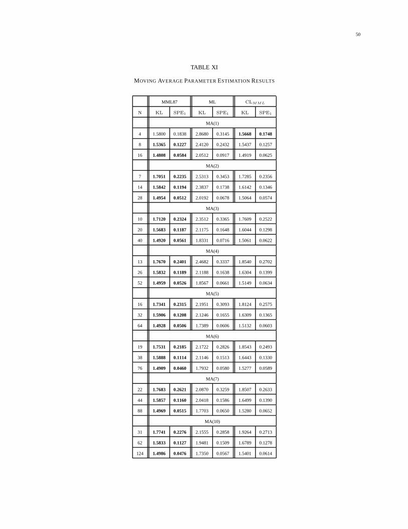
50
TABLE XI
MOVING AVERAGE PARAMETER ESTIMATION RESULTS
MML87 ML CLMML
N KL SPE1 KL SPE1 KL SPE1
MA(1)
4 1.5800 0.1838 2.8680 0.3145 1.5668 0.1748
8 1.5365 0.1227 2.4120 0.2432 1.5437 0.1257
16 1.4808 0.0584 2.0512 0.0917 1.4919 0.0625
MA(2)
7 1.7051 0.2235 2.5313 0.3453 1.7285 0.2356
14 1.5842 0.1194 2.3837 0.1738 1.6142 0.1346
28 1.4954 0.0512 2.0192 0.0678 1.5064 0.0574
MA(3)
10 1.7120 0.2324 2.3512 0.3365 1.7609 0.2522
20 1.5683 0.1187 2.1175 0.1648 1.6044 0.1298
40 1.4920 0.0561 1.8331 0.0716 1.5061 0.0622
MA(4)
13 1.7670 0.2401 2.4682 0.3337 1.8540 0.2702
26 1.5832 0.1189 2.1188 0.1638 1.6304 0.1399
52 1.4959 0.0526 1.8567 0.0661 1.5149 0.0634
MA(5)
16 1.7341 0.2315 2.1951 0.3093 1.8124 0.2575
32 1.5906 0.1208 2.1246 0.1655 1.6309 0.1365
64 1.4928 0.0506 1.7389 0.0606 1.5132 0.0603
MA(6)
19 1.7531 0.2185 2.1722 0.2826 1.8543 0.2493
38 1.5888 0.1114 2.1146 0.1513 1.6443 0.1330
76 1.4909 0.0460 1.7932 0.0580 1.5277 0.0589
MA(7)
22 1.7683 0.2621 2.0870 0.3259 1.8507 0.2633
44 1.5857 0.1160 2.0418 0.1586 1.6499 0.1390
88 1.4969 0.0515 1.7703 0.0650 1.5280 0.0652
MA(10)
31 1.7741 0.2276 2.1555 0.2858 1.9264 0.2713
62 1.5833 0.1127 1.9481 0.1509 1.6789 0.1278
124 1.4986 0.0476 1.7350 0.0567 1.5401 0.0614

51
TABLE XII
MA TEST SCORES ON SYNTHETIC DATA
Score MML87 AIC AICc BIC KICc
N = 10, P ∈ [1, 3]
KL1000 1.6387 2.9290 2.8698 2.9241 2.8227
SPE1 0.2024 0.3041 0.2457 0.2867 0.2474
L1 1.2132 1.3054 1.2537 1.2857 1.2705
N = 13, P ∈ [1, 4]
KL1000 1.6610 2.7178 2.7128 2.7478 2.7231
SPE1 0.2118 0.2991 0.2815 0.2868 0.2640
L1 1.2332 1.3434 1.3178 1.3286 1.2835
N = 16, P ∈ [1, 5]
KL1000 1.6565 2.5134 2.5014 2.5142 2.4673
SPE1 0.2076 0.2818 0.2609 0.2635 0.2559
L1 1.2592 1.3413 1.3070 1.3146 1.3211
N = 19, P ∈ [1, 6]
KL1000 1.6618 2.5783 2.5728 2.5754 2.6874
SPE1 0.2110 0.2830 0.2686 0.2651 0.2617
L1 1.2921 1.3465 1.3469 1.3453 1.3597
N = 22, P ∈ [1, 7]
KL1000 1.6869 2.6664 2.7252 2.6910 2.6527
SPE1 0.2254 0.2926 0.2694 0.2680 0.2668
L1 1.3158 1.3989 1.3613 1.3610 1.3696
N = 25, P ∈ [1, 8]
KL1000 1.6575 2.4339 2.4369 2.4222 2.6671
SPE1 0.2061 0.2631 0.2571 0.2472 0.2495
L1 1.3278 1.3947 1.3749 1.3704 1.3841
N = 31, P ∈ [1, 10]
KL1000 1.6751 2.4265 2.3688 2.3714 2.4586
SPE1 0.2012 0.2484 0.2341 0.2416 0.2488
L1 1.4195 1.5175 1.4485 1.4707 1.5041
N = 50, P ∈ [1, 10]
KL1000 1.5750 2.1617 2.0731 2.0140 2.0209
SPE1 0.1257 0.1691 0.1540 0.1539 0.1517
L1 1.2651 1.3700 1.3543 1.3099 1.3111

52
TABLE XIII
MA ORDER SELECTION RESULTS
MML87 AIC AICc BIC KICc
N < = > < = > < = > < = > < = >
10 569 397 34 489 428 83 593 384 23 517 422 61 674 321 5
13 593 355 52 533 361 106 611 337 52 574 353 73 673 306 21
16 631 308 61 543 327 130 649 300 51 629 308 63 723 265 12
19 659 278 63 582 290 128 670 258 72 666 267 67 730 238 32
22 671 280 49 578 298 124 663 281 56 685 275 40 737 241 22
25 680 276 44 591 284 125 687 255 58 711 258 31 754 230 16
31 671 268 61 573 288 139 673 255 72 725 234 41 754 222 24
50 555 386 59 397 398 205 490 390 120 622 354 24 610 357 33
53
VIII. CONCLUSION
This technical report has presented parameter and order estimation of Autoregressive and Moving
Average models within a Minimum Message Length framework. Suitable priors were examined and
expressions for the message lengths using the MML87 approximation were presented, and subsequently
tested on synthetic and real data sets. The results demonstrated that the MML87 criterion outperformed
the benchmark criteria against which it was compared in terms of both parameter estimation and overall
model selection (order and parameter estimation). Future work in consideration includes parameter and
order estimation of Autoregressive-Moving Average (ARMA) processes.
APPENDIX I
A CURVED PRIOR CORRECTION MODIFICATION
The Curved Prior Correction proposed by Wallace [2] has been modified to handle curved priors with
negative second derivatives of their negative log-likelihood (such as the Berger and Yang AR reference
prior (16)). Addition of these terms to the diagonals of the Fisher Information Matrix has the effect of
increasing the coding volume the more curved the prior becomes, and may in fact render the diagonal
terms negative if the prior is sufficiently curved. The entries of the modified curved prior correct Fisher
Information Matrix are given by
J(θi,θj)(θ) = Ey
[
∂2L(y|θ)
∂θi∂θj
]
+
∣
∣
∣
∣
∂2 log h(θ)
∂θi∂θj
∣
∣
∣
∣
(131)
which is differs from the original expression by adding the absolute of the curvature of the prior to
the expected curvature of negative log-likelihood. This has the effect of decreasing the coding volume
whenever the prior is curved, regardless of the sign of the curvature, and thus produces sensible results
in those cases when the second derivatives are negative.
APPENDIX II
AUTOREGRESSIVE MOVING-AVERAGE MODELS
Although this technical report focuses on pure Autoregressive and pure Moving Average models, this
appendix presents one MML87 formulation for mixed Autoregressive Moving Average (ARMA) models.
This work is confined to an appendix as the performance of the MML87 ARMA estimator has been only
briefly examined. The ARMA(P,Q) explanation of measurement yn is
P∏
i=1
(1−D−1pi)yn =
R∑
i=1
civn−i + vn (132)
54
where p are the process poles and D is the delay operator. The negative log-likelihood may be formed in a
similar fashion to the pure autoregressive process. The modelling error for a measurement yn conditioned
on P previous measurements of y is then
zn = yn +
P∑
i=1
aiyn−i (133)
However, in the case of the ARMA process the error sequence z is not a white noise sequence as per
the pure autoregression. Instead,
z ∼ MA(c, σ2) (134)
that is, it is distributed per a Moving Average process with coefficients c and innovation variance σ2. To
represent the resultant negative log-likelihood in matrix form, let xn = [yn−1, . . . , yn−P ] and form the
autoregression matrix as
Φ =[
xT(P+1), . . . ,x
TN
]
(135)
Including the unconditional term for the first P measurements, the complete negative log-likelihood is
given by
L(y|θ) =P
2log(2π) +
1
2log |Γ(θ)|+ 1
2y(1:P )Γ
−1(θ)yT(1:P )
+N − P
2log(2π) +
1
2log |W(c, σ2)|
+1
2
(
y(P+1:N) + aΦ)
W−1(c, σ2)(
y(P+1:N) + aΦ)T (136)
where Γ(θ) is the (P×P ) ARMA process autocovariance matrix, and W(c, σ2) is the (N−P )×(N−P )
Moving Average process autocovariance matrix. The model may be parametrised with the Autoregressive
parameters in root space, i.e. a ≡ a(β) as per Section IV, and the Moving Average parameters in
coefficient space as per Section V. In this case, priors for all model parameters may be selected from
Section III as appropriate. Using Whittle’s approximation as a basis, an asymptotic approximation of
the exact Information Matrix of the ARMA process can be found. Begin by defining two auxilliary
autoregressions
P∏
i=1
(1−D−1pi)rn = ρn (137)
sn +P∑
i=1
aisn−i = −ρn (138)
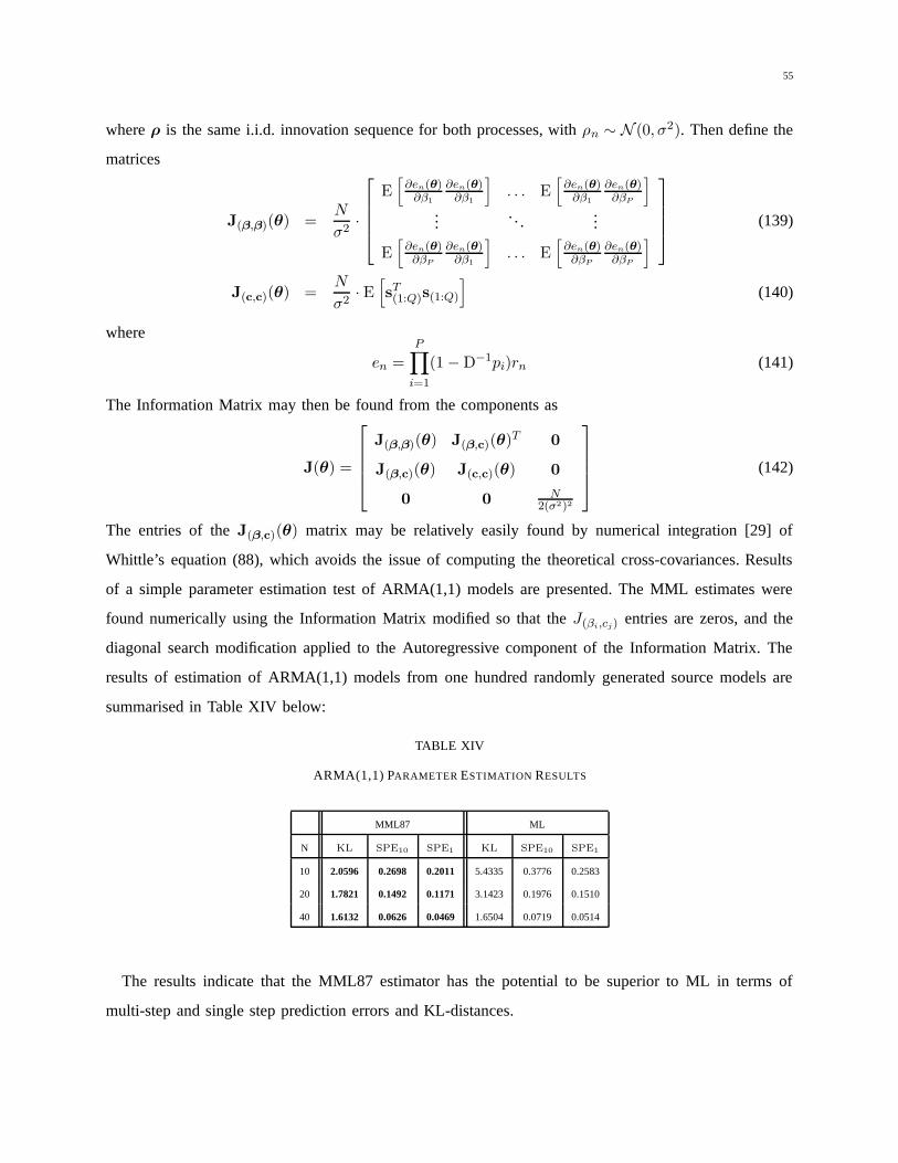
55
where ρ is the same i.i.d. innovation sequence for both processes, with ρn ∼ N (0, σ2). Then define the
matrices
J(β,β)(θ) =N
σ2·
E[
∂en(θ)∂β1
∂en(θ)∂β1
]
. . . E[
∂en(θ)∂β1
∂en(θ)∂βP
]
.... . .
...
E[
∂en(θ)∂βP
∂en(θ)∂β1
]
. . . E[
∂en(θ)∂βP
∂en(θ)∂βP
]
(139)
J(c,c)(θ) =N
σ2· E[
sT(1:Q)s(1:Q)
]
(140)
where
en =
P∏
i=1
(1−D−1pi)rn (141)
The Information Matrix may then be found from the components as
J(θ) =
J(β,β)(θ) J(β,c)(θ)T 0
J(β,c)(θ) J(c,c)(θ) 0
0 0 N2(σ2)2
(142)
The entries of the J(β,c)(θ) matrix may be relatively easily found by numerical integration [29] of
Whittle’s equation (88), which avoids the issue of computing the theoretical cross-covariances. Results
of a simple parameter estimation test of ARMA(1,1) models are presented. The MML estimates were
found numerically using the Information Matrix modified so that the J(βi,cj) entries are zeros, and the
diagonal search modification applied to the Autoregressive component of the Information Matrix. The
results of estimation of ARMA(1,1) models from one hundred randomly generated source models are
summarised in Table XIV below:
TABLE XIV
ARMA(1,1) PARAMETER ESTIMATION RESULTS
MML87 ML
N KL SPE10 SPE1 KL SPE10 SPE1
10 2.0596 0.2698 0.2011 5.4335 0.3776 0.2583
20 1.7821 0.1492 0.1171 3.1423 0.1976 0.1510
40 1.6132 0.0626 0.0469 1.6504 0.0719 0.0514
The results indicate that the MML87 estimator has the potential to be superior to ML in terms of
multi-step and single step prediction errors and KL-distances.
56
APPENDIX III
COMPUTING AUTOREGRESSIVE MOVING-AVERAGE LIKELIHOODS VIA THE KALMAN FILTER
For convenience the simple algorithm for computing the negative log-likelihood of an Autoregressive
Moving Average process efficiently via the Kalman Filter [42] is presented here. For an ARMA(P,Q)
process there is the P -vector of autoregressive coefficients a, the Q-vector of moving average coefficients
c, and the process innovation variance. The algorithm begins by formulating the model in a state-space
representation. Define m as
m = max P,Q (143)
and then augment the parameter vectors
α =[
a,0(m−P )
]
(144)
β =[
1, c,0(m−Q)
]
(145)
Then define the matrices
F =
αT IQ
0 0Q
(146)
Q = σ2βT β (147)
H = [1,0m] (148)
where 0Q is a Q long row vector of zeros, F is the state-transition matrix, Q is the process noise
covariance matrix, and H is the observation matrix. The likelihood may be computed using the famed
Kalman Filter recursive equations. At step n, first compute the predictions
X(n|n−1) = F ·X(n−1|n−1) (149)
P(n|n−1) = F ·P(n−1|n−1) · F + Q (150)
yn = H ·X(n|n−1) (151)
From this, the innovations may be estimated
vn = yn − yn (152)
σ2n = H ·P(n|n−1) ·HT (153)
57
The update equations are evaluated next:
Kn = P(n|n−1) ·HT · σ−2n (154)
X(n|n) = X(n|n−1) + Knvn (155)
P(n|n) = P(n|n−1) −K ·H ·P(n|n−1) (156)
This process is repeated for all data in y, i.e. for n = 1 . . . N ; the negative-log likelihood may then be
found as
L(y|a, c, σ2) =N
2log(2π) +
1
2
N∑
n=1
log σ2n +
1
2
N∑
n=1
v2n
σ2n
(157)
Clearly, as N grows larger this algorithm becomes much more efficient than direct computation of the
likelihood via inversion of the autocovariance matrix. The only issue that remains is to initialise the
algorithm, i.e. appropriate selection of X(0|0) and P(0|0). An algorithm is given in [43] to compute these
starting values so that the recursions will yield the exact negative log-likelihood. This algorithm selects
X(0|0) = 0(m+1) (158)
S = I(m2) −F⊗ F (159)
P(0|0) = S−1 · vec(Q) (160)
where ⊗ denotes the Kronecker product, and vec(A) builds a column vector by stacking the columns of
A. One point to note is that the paper from which the initialisation algorithm was taken [43] seems to
possess a small error, and incorrectly transposes the second F in (159) (equation 12 in the cited paper).
REFERENCES
[1] G. E. P. Box, G. M. Jenkins, and G. C. Reinsel, Time Series Analysis: Forecasting and Control. Englewood Cliffs, New
Jersey: Prentice Hall, 1994.
[2] C. S. Wallace, Statistical and Inductive Inference by Minimum Message Length. Berlin, Germany: Springer, 2005.
[3] P. M. T. Broersen and S. de Waele, “Empirical time series analysis and maximum likelihood estimation,” in IEEE Benelux
Signal Processing Symposium, 2000, pp. 1–4.
[4] J. P. Burg, “Maximum entropy spectral analysis,” in Proc.37th Meet. Soc. Explorational Geophys., Oklahoma City, OK,
1967.
[5] L. Ljung, System identification (2nd ed.): theory for the user. Upper Saddle River, NJ, USA: Prentice Hall, 1999.
[6] K. Astrom, “Maximum likelihood and prediction error methods,” Automatica, vol. 16, pp. 551–574, 1980.
[7] T. Soederstroem and P. Stoica, System identification. Hemel Hempstead, UK: Prentice Hall, 1989.
[8] C. S. Wallace and D. M. Boulton, “An information measure for classification,” Computer Journal, vol. 11, pp. 185–194,
August 1968.
58
[9] H. Akaike, “A new look at the statistical model identification,” IEEE Transactions on Automatic Control, vol. 19, no. 6,
1974.
[10] C. M. Hurvich and C. Tsai, “Regression and time series model selection in small samples,” Biometrika, vol. 76, pp.
297–307, 1989.
[11] G. Schwarz, “Estimating the dimension of a model,” Annals of Statistics, vol. 6, pp. 461–464, 1978.
[12] J. E. Cavanaugh, “A large-sample model selection criterion based on Kullback’s symmetric divergence,” Statist. Probability
Lett., vol. 42, pp. 333–343, 1999.
[13] A. Seghouane and M. Bekara, “A small sample model selection criterion based on Kullback’s symmetric divergence,”
IEEE Transactions on Signal Processing, vol. 52, no. 12, pp. 3314–3323, 2004.
[14] J. Rissanen, “Modeling by shortest data description,” Automatica, vol. 14, pp. 465–471, 1978.
[15] ——, “Fisher information and stochastic complexity,” IEEE Transactions on Information Theory, vol. 42, no. 1, pp. 40–47,
1996.
[16] ——, “A predictive-least squares principle,” IMA J. Math. Contr. Inform., vol. 3, pp. 211–222, 1986.
[17] M. Wax, “Order selection for ar models by predictive least squares,” IEEE Transactions on Acoustics, Speech and Signal
Processing, vol. 36, pp. 581–588, 1988.
[18] P. M. T. Broersen, “Finite sample criteria for autoregressive order selection,” IEEE Transactions on Signal Processing,
vol. 48, no. 2, pp. 3550–3558, 2000.
[19] P. M. Djuric and S. M. Kay, “Order selection of autoregressive models,” IEEE Transactions on Signal Processing, vol. 40,
no. 11, pp. 2829–2833, 1992.
[20] C. S. Wallace and D. M. Boulton, “An invariant Bayes method for point estimation,” Classification Society Bulletin, vol. 3,
no. 3, pp. 11–34, 1975.
[21] C. S. Wallace and P. R. Freeman, “Estimation and inference by compact coding,” J. Royal Statistical Society B, vol. 49,
pp. 240–252, 1987.
[22] G. E. Farr and C. S. Wallace, “The complexity of Strict Minimum Message Length inference,” Computer Journal, vol. 45,
no. 3, pp. 285–292, 2002.
[23] L. J. Fitzgibbon, D. L. Dowe, and L. Allison, “Message from Monte Carlo,” School of Computer Science and Software
Engineering, Monash University, Australia 3800, Tech Report 2002/107, Decemember 2002.
[24] G. Huerta and M. West, “Priors and component structures in autoregressive time series models,” Journal of the Royal
Statistical Society, Series B, vol. 61, no. 4, pp. 881–899, 1999.
[25] P. Infer, Yang, and R. Berger, “A catalog of noninformative priors,” 1997. [Online]. Available:
citeseer.ist.psu.edu/yang96catalog.html
[26] J. Marriot and P. Newbold, “The strength of evidence for unit autoregressive roots and structural breaks: A bayesian
perspective,” Journal of Econometrics, vol. 98, p. 1, 2000.
[27] R. S. Ehlers and S. P. Brooks, “Bayesian analyis of order uncertainty in ARIMA models,” Federal University of Parana,
Tech. Rep. 2004/05-B, 2004.
[28] P. C. B. Phillips, “To criticize the critics: an objective Bayesian analysis of stochastic trends,” Journal of Applied
Econometrics, vol. 6, pp. 333–364, 1991.
[29] I. N. Bronshtein, K. A. Semendyayev, G. Musiol, and H. Muehlig, Handbook of Mathematics. Springer Verlag, 2003.
[30] D. Piccolo, “The size of the stationarity and invertibility region of an autoregressive-moving average process,” Journal of
Time Series Analysis, vol. 3, no. 4, pp. 245–247, 1982.
59
[31] L. J. Fitzgibbon, D. L. Dowe, and F. Vahid, “Minimum message length autoregressive model order selection,” in Proceedings
of the International Conference on Intelligent Sensing and Information Processing, Chennai, India, January 2004, pp. 439–
444.
[32] M. Sak, D. L. Dowe, and F. Vahid, “Minimum message length moving average time series data mining,” in Proceedings
of the First International ICSC Symposium on Advanced Computing in Financial Markets (ACFM2005), Istanbul, Turkey,
December 15-17 2005.
[33] B. Porat and B. Friedlander, “Computation of the exact information matrix of gaussian time series with stationary random
components,” IEEE Transactions on Acoustics, Speech and Signal Processing, vol. 34, no. 1, pp. 118–130, 1986.
[34] M. Karanasos, “A new method for obtaining the autocovariance of an ARMA model: An exact form solution,” Econometric
Theory, vol. 14, pp. 622–640, 1998.
[35] P. Whittle, “The analysis of multiple stationary time series,” Journal of the Royal Statistical Society, vol. 15, pp. 125–139,
1953.
[36] W. Huyer and A. Neumaier, “Global optimization by multilevel coordinate search,” Global Optimization, vol. 14, pp.
331–355, 1999.
[37] O. Barndorff-Nielsen and G. Schou, “On the parametrization of autoregressive models by partial autocorrelations,” Journal
of Multivariate Analysis, vol. 3, pp. 408–419, 1973.
[38] J. F. Monahan, “A note on enforcing stationarity in autoregressive-moving average models,” Biometrika, vol. 71, pp.
403–404, 1984.
[39] J. Rissanen, “MDL denoising,” IEEE Transactions on Information Theory, vol. 46, no. 7, pp. 2537–2543, 2000.
[40] ——, “An introduction to the MDL principle.” [Online]. Available: http://www.mdl-
research.org/jorma.rissanen/pub/Intro.pdf
[41] M. C. Jones, “Randomly choosing parameters from the stationarity and invertibility regions of autoregressive-moving
average models,” Applied Statistics, vol. 36, no. 2, pp. 134–138, 1987.
[42] R. E. Kalman, “A new approach to linear filtering and prediction problems,” Transactions of the ASME–Journal of Basic
Engineering, vol. 82, no. Series D, pp. 35–45, 1960.
[43] G. Gardner, A. C. Harvey, and G. D. A. Phillips, “Algorithm AS154: An algorithm for exact maximum likelihood estimation
of autoregressive-moving average models by means of kalman filtering,” Applied Statistics, vol. 29, pp. 311–322, 1980.