DeepMag: Source Specific Motion MagnificationUsing Gradient Ascent

Weixuan Chen1 and Daniel McDuff2

1Massachusetts Institute of Technology, Cambridge, Massachusetts2Microsoft Research, Redmond, Washington

June 2018

Abstract

Many important physical phenomena involve subtle signals that are difficult to observe withthe unaided eye, yet visualizing them can be very informative. Current motion magnificationtechniques can reveal these small temporal variations in video, but require precise prior knowl-edge about the target signal, and cannot deal with interference motions at a similar frequency.We present DeepMag an end-to-end deep neural video-processing framework based on gradientascent that enables automated magnification of subtle color and motion signals from a specificsource, even in the presence of large motions of various velocities. While the approach is gen-eralizable, the advantages of DeepMag are highlighted via the task of video-based physiologicalvisualization. Through systematic quantitative and qualitative evaluation of the approach onvideos with different levels of head motion, we compare the magnification of pulse and respirationto existing state-of-the-art methods. Our method produces magnified videos with substantiallyfewer artifacts and blurring whilst magnifying the physiological changes by a similar degree.

1 IntroductionRevealing subtle signals in our everyday world is important for helping us understand the processesthat cause them. Magnifying small temporal variations in video has applications in both basicscience (e.g., visualizing physical processes in the world), engineering (e.g., identifying the motionof large structures) and education (e.g, teaching scientific principals). To provide an illustration,physiological phenomena are often invisible to the unaided eye, yet understanding these processes canhelp us detect and treat negative health conditions. Pulse and respiration magnification specifically,are good exemplar tasks for video magnification as physiological phenomena cause both subtle colorand motion variations. Furthermore, larger rigid and non-rigid motions of the body often mask thesubtle variations, which makes the magnification of physiological signals non-trivial.

Several methods have been proposed to reveal subtle temporal variations in video. Lagrangianmethods for video magnification [15] rely on accurate tracking of the motion of particles (e.g., viaoptical flow) over time. These approaches are computationally expensive and will not work effectivelyfor color changes. Eulerian video magnification methods do not rely on motion estimation, but rather

1

arX

iv:1

808.

0333

8v1

[cs

.CV

] 9

Aug

201

8

+

Motion

Representation

Motion

Representation

Input Video Example Frames

Input Video Scanline

Eulerian Video Magnification Result

DeepMag Result

Band-pass

FilteringRecon-

struction

Convolutional

Neural Network

Recon-

struction

Gradient Ascent

Previous Approaches

Our

Approach

Figure 1: We present a novel end-to-end deep neural framework for video magnification. Our methodallows measurement, magnification and synthesis of subtle color and motion changes from a specificsource even in the presence of large motions. We demonstrate this via pulse and respiration ma-nipulation in 2D videos. Our approach produces magnified videos with substantially fewer artifactswhen compared to the state-of-the-art.

magnify the variation of pixel values over time [42]. This simple and clever approach allows for subtlesignals to be magnified that might otherwise be missed by optical flow. Subsequent iterations of suchapproaches have improved the method with phase-based representations [36], matting [4], second-order manipulation [44], and learning-based representations [22]. However, all these approaches usefrequency properties to separate the target signal from noise, so they require precise prior knowledgeabout the signal frequency. Furthermore, if the signal of interest is at a similar frequency to anothersignal (for example if head motions are at a similar frequency as the pulse signal) an Eulerianapproach will magnify both and cause numerous artifacts (see Fig. 1).

To address these problems, we present a generalized approach for magnifying color and motionvariations in videos that feature other periodic or random motions. Our method leverages a convo-lutional neural network (CNN) as a video motion discriminator to separate a specific source signaleven if it overlaps with other motion sources in the frequency domain. Then the separated signalcan be magnified in video by performing gradient ascent [5] in the input space of the CNN, withthe other motion sources untouched. To adapt the gradient ascent method to the video magnifica-tion task, several methodological innovations are introduced including adding L1 normalization andsign correction. The whole algorithm proves to work effectively even in the presence of interferencemotions with large magnitudes and velocities. Fig. 1 shows a comparison between the proposedmethod and previous approaches.

While our method can generally be applied to any type of color or motion magnification task,magnifying physiological changes on the human body without impacting other aspects of the visualappearance is an especially interesting use case with numerous applications in and of itself. Inmedicine and affective computing the photoplethysmogram (PPG) and respiration signals are usedas unobtrusive measures of cardiopulmonary performance. Visualizing these signals could help in theunderstanding vascular disease, heart conditions (e.g., arterial fibrillation) [2] and stress responses.For example, jugular venous pressure (JVP) is analyzed by studying subtle motions of the neck. Thisis challenging for clinicians and video-magnification could offer a practical aid. Another application

2

is in the design of avatars [30]. Synthetic embodied agents may fall into the “uncanny valley” [21]or be easily detected as “spoofs” if they do not exhibit accurate physiological responses, includingrespiration, pulse rates and blood flow that can be recovered using video analysis [26]. Our methodpresents the opportunity to not only magnify signals but also synthesize them at different frequencieswithin a video.

The main contributions of this paper are to: (1) present our novel end-to-end framework for videomagnification based on a deep convolutional neural network and gradient ascent, (2) demonstraterecovery of the pulse and respiration waves and magnification of these signals in the presence oflarge rigid head motions, (3) systematically quantitatively and qualitatively compare our approachwith state-of-the-art motion magnification approaches under different rigid motion conditions.

2 Related Work

2.1 Video Motion MagnificationLagrangian video magnification approaches involve estimation of motion trajectories that are thenamplified [15, 38]. However, these approaches require a number of complex steps including, per-forming a robust registration, frame intensity normalization, tracking and clustering of feature pointtrajectories, segmentation and magnification. Another approach, using temporal sampling kernelscan aid visualization of time-varying effects within videos [8]. However, this method involves videodownsampling and relies on high framerate input videos.

The neat Eulerian video magnification (EVM) approach proposed by Wu et al. [42] combines spa-tial decomposition with temporal filtering to reveal time varying signals without estimating motiontrajectories. However, it uses linear magnification that only allows for relatively small magnificationsat high spatial frequencies and cannot handle spatially variant magnification. To counter the limita-tion, Wadhwa et al. [36] proposed a non-linear phase-based approach, magnifying phase variations ofa complex steerable pyramid over time. Replacing the complex steerable pyramid [36] with a Rieszpyramid [37] produces faster results. In general, the linear EVM technique is better at magnify-ing small color changes, while the phase-based pipeline is better at magnifying subtle motions [41].Both the EVM and the phase-EVM techniques rely on hand-crafted motion representations. Tooptimize the representation construction process, a learning-based method [22] was proposed, whichuses convolutional neural networks as both frame encoders and decoders. With the learned motionrepresentation, fewer ringing artifacts and better noise characteristics have been achieved.

One common problem with all the methods above is that they are limited to stationary objects,whereas many realistic applications would involve small motions of interest in the presence of largeones. After motion magnification, these large motions would result in large artifacts such as haloes orripples, and overwhelm any small temporal variation. A couple of improvements have been proposedincluding a clever layer-based approach called DVMAG [4]. By using matting, it can amplify onlya specific region of interest (ROI) while maintaining the quality of nearby regions of the image.However, the approach relies on 2D warping (either affine or translation-only) to discount largemotions, so it is only good at diminishing the impact of motions parallel to the camera plane andcannot deal with more complex 3D motions such as the human head rotation. The other methodaddressing large motion interferences is video acceleration magnification (VAM) [44]. It assumeslarge motions to be linear on the temporal scale so that magnifying the motion acceleration via asecond-order derivative filter will only affect small non-linear motions. However, the method will

3

fail if the large motions have any non-linear components, and ideal linear motions are rare in reallife, especially on living organisms.

Another problem with all the previous motion magnification methods is that they use frequencyproperties to separate target signals from noise, so they typically require the frequency of interestto be known a priori for the best results and, as such, have at least three parameters (the frequencybounds and a magnification factor) that need to be tuned. If there are motion signals from differentsources that are at similar frequencies (e.g., someone is breathing and turning their head), it ispreviously not possible to isolate the different signals.

2.2 Gradient Ascent for Feature VisualizationOpposite to gradient descent, gradient ascent is a first-order iterative optimization algorithm thattakes steps proportional to the positive of the gradient (or approximate gradient) of a function. Sinceneural networks are generally differentiable with respect to their inputs, it is possible to performgradient ascent in the input space by freezing the network weights and iteratively tweaking theinputs towards the maximization of an internal neuron firing or the final output behavior. Earlyworks found that this technique can be used to visualize network features (showing what a networkis looking for by generating examples) [5, 29] and to produce saliency maps (showing what part ofan example is responsible for the network activating a particular way) [29].

A recent famous application of gradient ascent in feature visualization is Google DeepDream [20].It maximizes the L2 norm of activations of a particular layer in a CNN to enhance patterns inimages and create a dream-like hallucinogenic appearance. It should be noted that applying gradientascent independently to each pixel of the inputs commonly produces images with nonsensical high-frequency noise, which can be improved by including a regularizer that prefers inputs that havenatural image statistics. Also, following the same idea of DeepDream, not only a network layer butalso a single neuron, a channel, or an output class can be set as the objective of gradient ascent.For a comprehensive discussion of various regularizers and different optimization objectives used infeature visualization tasks see [23].

None of the previous works have applied gradient ascent to motion magnification or any taskrelated to motions in video. In contrast to DeepDream and similar visualization tools, our methodmaximizes the output activation of a CNN in motion representations computed from frames insteadof in raw images.

2.3 Video-Based Physiological MeasurementOver the past decade video-based physiological measurement using RGB cameras has developedsignificantly [18]. For instance, physiological parameters such as heart rate (HR) and breathing rate(BR) have been accurately extracted from facial videos in which subtle color changes of the skincaused by blood circulation can be amplified and analyzed (a.k.a., imaging plethysmography) [35, 26,25, 10, 33, 40]. Similar metrics have also been extracted by analyzing subtle face motions associatedwith the blood ejection into the vessels (a.k.a., imaging ballistocardiography) [1] as well as moreprominent chest volume changes during breathing [32, 12].

Early work on imaging plethysmography identified that spatial averaging of skin pixel valuesfrom an imager could be used to recover the blood volume pulse [31]. The strongest pulse signal wasobserved in the green channel [35], but a combination of color channels provides improved results [26,

4

C(t)

...p(t) ... p(t+4) ...

Motion RepresentationInput Video Predicted Motion Signal

X1(t)C(t+1)

Convolutional Neural Network

C(t) C(t+1)

Xn(t) Xn+1(t)

Output Video

Gradient w.r.t. Xn(t)

y(t) = p(t+1) - p(t)

Reconstruction

Sign Correction L1 Normalization

+

XN (t)

θ

γ∇||y(Xn|θ)||2

...~ ~

Figure 2: The architecture of DeepMag. The CNN model predicts the motion signal of interestbased on a motion representation computed from consecutive video frames. Magnification of themotion signal in video can be achieved by amplifying the L2 norm of its first-order derivative andthen propagating the changes back to the motion representation using gradient ascent.

17]. Combining these insights with face tracking and signal decomposition enables a fully automatedrecovery of the pulse wave and heart rate [26].

In the presence of dynamic lighting and motion, advancements were needed to successfully recoverthe pulse signal. Leveraging models grounded in the optical properties of the skin has improvedperformance. The CHROM [10] method uses a linear combination of the chrominance signals. Itmakes the assumption of a standardized skin color profile to white-balance the video frames. ThePulse Blood Vector (PBV) method [11] relies on characteristic blood volume changes in differentregions of the frequency spectrum to weight the color channels. Adapting the facial ROI can improvethe performance of iPPG measurements as blood perfusion varies in intensity across the body [34]

Few approaches have made use of supervised learning for video-based physiological measure-ment. Formulating the problem is not trivial and performance has been modest [24, 19]. Recentadvances in deep neural video analysis offer opportunities for recovering accurate physiological mea-surements. Recently, Chen and McDuff [3] presented a supervised method using a convolutionalattention network that provided state-of-the-art measurement performance and generalized acrosspeople. Our video magnification algorithm is based on a novel framework that allows recovery ofpulse and respiratory waves using such a convolutional architecture.

3 Methods

3.1 Video Magnification Using Gradient AscentFig. 2 shows the workflow of the proposed video magnification algorithm using gradient ascent.Similar to previous video magnification algorithms, it reads a series of video frames C(t), t =1, 2, · · · , T , magnifies a specific subtle motion in them, and outputs frames of the same dimension

5

C(t), t = 1, 2, · · · , T .The first step of our algorithm is computing the input motion representation X1(t) from the

original video frames C(t), t = 1, 2, · · · , T . X1(t) represents any change happening between twoconsecutive frames C(t) and C(t + 1). Common motion representations include frame differenceand optical flow. Different motion representations can emphasize different aspects of motions. Forexample, the physio-logy-based motion representation called normalized frame difference [3] wasproposed to capture skin absorption changes robustly under varying rigid motions. On the otherhand, optical flow based on the brightness constancy constraint is good at representing object dis-placements, but largely ignores the light absorption changes of objects. As a general framework forvideo magnification, our algorithm supports any type of motion representation.

In realistic videos the motion representations are comprised of multiple motions from differentsources. For example, unconstrained facial video recordings commonly contain not only respirationmovements and pulse-induced skin color changes but also head rotations and facial expressions.As we are only interested in magnifying one of these motions at a time, a video magnificationalgorithm should have the ability to separate the target motion from the others in the motionrepresentation. Previous methods have typically used frequency-domain characteristics of the targetmotion in separation, so they rely on precise prior knowledge about the motion frequency (e.g. theexact heart rate). Furthermore, if any other motion overlaps with the target motion in frequency,it will still be magnified and cause artifacts. To improve the specificity of magnification and reducethe dependence on prior knowledge, we propose to use a deep convolutional neural network (CNN)to model the relationship between the motion representation and the motion of interest. As shownin Fig. 2, the CNN has the input motion representation X1(t) as its input, and the first-orderderivative y(t) of the target motion signal p(t) as its output. For many motion types, there areavailable datasets with paired videos and ground truth motion signals (e.g., facial videos with pulseand respiration signals measured from medical devices). Therefore, the weights θ of the CNN can bedetermined by training it on one of these datasets. It has been shown in [3] that CNNs trained in thisway have good generalization ability over different objects (human subjects), different backgrounds,and different lighting conditions.

As the CNN has established the relationship between the input motion representation X1(t) andthe target motion signal p(t), magnification of p(t) in X1(t) can be achieved by amplifying the L2norm of its first-order derivative y(t) and then propagating the changes back to X1(t) using gradientascent. The process can be expressed as

Xn+1 = Xn + γ∇‖y(Xn|θ)‖2, n = 1, 2, · · · , N − 1 (1)

in which N is the total number of iterations and γ is the step size. θ is the weights of the CNN,which are frozen during gradient ascent. ∇‖y(Xn|θ)‖2 is the gradient of ‖y(t)‖2 with respect toXn(t), which is the direction to which Xn(t) can be modified to specifically magnify the targetmotion rather than the other motions. Note that both Xn and y correspond to time point t in (1),but t is omitted for conciseness.

The vanilla gradient ascent in (1) is appropriate for magnifying a single motion representationX1(t) at time t. However, for video magnification, a series of motion representations X1(t), t =1, 2, · · · , T need to be processed and magnified to the same level. Since the magnitude of the gradientis sensitive to the surface shape of the objective function (i.e. a point on a steep surface will have highmagnitude whereas a point on the fairly flat surface will have low magnitude), it is not guaranteedthat the accumulated gradient will be proportional to the original motion amplitude. Therefore, we

6

apply L1 normalization to the gradient

Xn+1 = Xn + γ∇‖y(Xn|θ)‖2

‖∇‖y(Xn|θ)‖2‖1(2)

so that only the gradient direction is kept and the gradient magnitude is controlled by the step sizeγ.

Another problem with (1) is that motions in opposite directions contribute equivalently to the L2norm of y(t). As a result, the target motion might be amplified in terms of the absolute amplitudebut 180-degrees out of phase. To address the problem, we correct the signs of the gradient to alwaysmatch the signs of the input motion representation

Xn+1 = Xn + γ∇‖y(Xn|θ)‖2 � sgn(Xn �∇‖y(Xn|θ)‖2)

‖∇‖y(Xn|θ)‖2‖1(3)

in which sgn(·) is the sign function and � is element-wise multiplication.Summing up the changes of Xn(t) in all the iterations, we get the final expression of the magnified

motion representation:

XN = X1 +N−1∑n=1

γ∇‖y(Xn|θ)‖2 � sgn(Xn �∇‖y(Xn|θ)‖2)

‖∇‖y(Xn|θ)‖2‖1(4)

There are only two hyper-parameters γ and N , which can be tuned to change the magnificationfactor. Finally, the magnified motion representation can be combined with previous frames toiteratively generate the output video. The complete algorithm is summarized in Algorithm 1.

Algorithm 1 DeepMag video magnificationRequire: C(t), t = 1, 2, · · · , T is a series of video frames, M is a motion representation estimator,

θ is the pre-trained CNN weights for predicting a target motion signal y, γ is the step size, andN is the number of iterations

1: for t = 1 to T − 1 do2: Compute motion representation: X1(t)←M(C(t), C(t+ 1))3: for n = 1 to N − 1 do4: Compute gradient: Gn(t)← ∇‖y(Xn(t)|θ, t)‖25: L1 normalization: Gn(t)← Gn(t)/‖Gn(t)‖16: Sign correction: Gn(t)← Gn(t)� sgn(Gn(t)�Xn(t))7: Gradient ascent: Xn+1(t)← Xn(t) + γGn(t)8: end for9: end for

10: C(1) = C(1)11: for t = 1 to T − 1 do12: Reconstruct magnified frame C(t+ 1)←M−1(C(t), XN (t))13: end for14: return C(t), t = 1, 2, · · · , T

7

3x3 conv, 32

Dimension:

3x3 conv, 32

Dimension:

36x36

3x3 conv, 32

123x123

3x3 conv, 32

2x2 pool 2x2 pool

0.25 dropout

Dimension:

3x3 conv, 64Dimension:

3x3 conv, 64

61x61

3x3 conv, 6418x18

3x3 conv, 64 2x2 pool

2x2 pool

Dimension:

3x3 conv, 128

0.25 dropout

30x30

3x3 conv, 128Dimension:

fc, 128 2x2 pool9x9

0.5 dropout 0.25 dropout

fc, 1

Dimension:

3x3 conv, 12815x15

3x3 conv, 128

2x2 pool

0.25 dropoutDimension:

fc, 2567x7

0.5 dropout

fc, 1

Input

36x36x3

(a)

Input

123x123x4

(b)

Figure 3: We used two exemplar tasks to illustrate the benefits of DeepMag. a) Color (Blood flow)magnification. b) Motion (respiration) magnification. These two tasks require different input motionrepresentations and CNN architectures due to the nature of the motion signals.

3.2 Example I: Color MagnificationOne example of applying our proposed algorithm is in the magnification of subtle skin color changesassociated with the cardiac cycle. As blood flows through the skin it changes the light reflected fromit. A good motion representation for these color changes is normalized frame difference [3], which issummarized below.

For modeling lighting, imagers and physiology, previous works used the Lambert-Beer law (LBL)[14, 43] or Shafer’s dichromatic reflection model (DRM) [40]. We build our motion representationon top of the DRM as it provides a better framework for separating specular reflection and diffusereflection. Assume the light source has a constant spectral composition but varying intensity. Wecan define the RGB values of the k-th skin pixel in an image sequence by a time-varying function:

CCCk(t) = I(t) · (vvvs(t) + vvvd(t)) + vvvn(t) (5)

where CCCk(t) denotes a vector of the RGB values; I(t) is the luminance intensity level, which changeswith the light source as well as the distance between the light source, skin tissue and camera; I(t)is modulated by two components in the DRM: specular reflection vvvs(t), mirror-like light reflectionfrom the skin surface, and diffuse reflection vvvd(t), the absorption and scattering of light in skin-tissues; vvvn(t) denotes the quantization noise of the camera sensor. I(t), vvvs(t) and vvvd(t) can all bedecomposed into a stationary and a time-dependent part through a linear transformation [40]:

vvvd(t) = uuud · d0 + uuup · p(t) (6)

8

where uuud denotes the unit color vector of the skin-tissue; d0 denotes the stationary reflection strength;uuup denotes the relative pulsatile strengths caused by hemoglobin and melanin absorption; p(t) de-notes the BVP.

vvvs(t) = uuus · (s0 + s(t)) (7)

where uuus denotes the unit color vector of the light source spectrum; s0 and s(t) denote the stationaryand varying parts of specular reflections.

I(t) = I0 · (1 + i(t)) (8)

where I0 is the stationary part of the luminance intensity, and I0 · i(t) is the intensity variationobserved by the camera. The stationary components from the specular and diffuse reflections canbe combined into a single component representing the stationary skin reflection:

uuuc · c0 = uuus · s0 + uuud · d0 (9)

where uuuc denotes the unit color vector of the skin reflection and c0 denotes the reflection strength.Substituting (6), (7), (8) and (9) into (5), produces:

CCCk(t) = I0 · (1 + i(t)) · (uuuc · c0 + uuus · s(t) + uuup · p(t)) + vvvn(t) (10)

As the time-varying components are much smaller (i.e., orders of magnitude) than the stationarycomponents in (10), we can neglect any product between varying terms and approximate ccck(t) as:

CCCk(t) ≈ uuuc · I0 · c0 · (1 + i(t)) + uuus · I0 · s(t) + uuup · I0 · p(t) + vvvn(t) (11)

The first step in computing our motion representation is spatial averaging of pixels, which has beenwidely used for reducing the camera quantization error vvvn(t) in (11). We implemented this bydownsampling every frame to L pixels by L pixels using bicubic interpolation. Emperical evidenceshows that bicubic interpolation preserves the color information more accurately than linear in-terpolation [16]. Selecting L is a trade-off between suppressing camera noise and retaining spatialresolution ([39] found that L = 36 was a good choice for face videos.) The downsampled pixel valueswill still obey the DRM model only without the camera quantization error:

CCCl(t) ≈ uuuc · I0 · c0 + uuuc · I0 · c0 · i(t) + uuus · I0 · s(t) + uuup · I0 · p(t) (12)

where l = 1, · · · , L2 is the new pixel index in every frame.Then we need to reduce the dependency of CCCl(t) on the stationary skin reflection color uuuc · I0 · c0,

resulting from the light source and subject’s skin tone. In (12), uuuc ·I0 ·c0 appears twice. It is difficultto eliminate the second term as it interacts with the unknown i(t). However, the first time-invariantterm, which is usually dominant, can be removed by taking the first order derivative of both sidesof (12) with respect to time:

CCC ′l(t) ≈ uuuc · I0 · c0 · i′(t) + uuus · I0 · s′(t) + uuup · I0 · p′(t) (13)

One problem with this frame difference representation is that the stationary luminance intensitylevel I0 is spatially heterogeneous due to different distances to the light source and uneven skincontours. The spatial distribution of I0 has nothing to do with physiology, but is different in every

9

video recording setup. Thus, CCC ′l(t) was normalized by dividing it by the temporal mean of CCCl(t) toremove I0:

CCC ′l(t)CCCl(t)

≈ 111 · i′(t) + diag−1(uuuc)uuus ·s′(t)c0

+ diag−1(uuuc)uuup ·p′(t)c0

(14)

where 111 = [1 1 1]T . In (14), CCCl(t) needs to be computed pixel-by-pixel over a short time windowto minimize occlusion problems and prevent the propagation of errors. We found it was feasible tocompute it over two consecutive frames so that (14) can be expressed discretely as:

XXX1(l, t) = CCC ′l(t)CCCl(t)

∼ CCCl(t+ 1)−CCCl(t)CCCl(t+ 1) +CCCl(t)

(15)

which is the normalized frame difference we used as motion representation.The CNN we used for extracting pulse signals from the motion representation is shown in Fig.

3 (a). The pooling layers are 2x2 average pooling, and the convolution layers have a stride of one.All the layers use ReLU as the activation function. Note that bounded activation function such astanh and sigmoid are not suitable for this task, as they will limit the extent to which the motionrepresentation can be magnified in the gradient ascent.

After gradient ascent, the input motion representation XXX1(l, t) was magnified as XXXN (l, t), fromwhich we could reconstruct the magnified video. The first step of reconstruction is to denoise theoutput motion representation by filtering the accumulated gradient:

XXXN (l, t) = XXX1(l, t) + F(XXXN (l, t)−XXX1(l, t)) (16)

in which F is a zero-phase band-pass filter. Note that unlike previous motion magnification methodsthe function of the filter here is not to select the target motion but to remove low and high frequencynoise, so the filter bands do not need to precisely match the motion frequency in the video and canbe chosen conservatively. Specifically, a 6th-order Butterworth filter with cut-off frequencies of 0.7and 2.5 Hz was used to generally cover the normal heart rate range (42 to 150 beats per minute).Then we applied the inverse operation of (15) to reconstruct the downsampled version of the framesCCCl(t):

CCCl(t+ 1) = 1 + XXXN (l, t)1− XXXN (l, t)

· CCCl(t), CCCl(1) = CCCl(1) (17)

Finally, CCCl(t) was upsampled back to the original video resolution:

CCCk(t) = CCCk(t)− U(CCCl(t)) + U(CCCl(t)) (18)

in which U is an image upsampling operator.

3.3 Example II: Motion MagnificationOur second example is amplifying subtle motions on the human body induced by respiration. Weused phase variations in a complex steerable pyramid to represent the local motions in a video. Thecomplex steerable pyramid [28, 27] is a filter bank that breaks each frame of the video C(t) intocomplex-valued sub-bands corresponding to different scales and orientations. The basis functionsof this transformation are scaled and oriented Gabor-like wavelets with both cosine- and sine-phasecomponents. Each pair of cosine- and sine-like filters can be used to separate the amplitude of local

10

wavelets from their phase. Specifically, each scale r and orientation θ is a complex image that canbe expressed in terms of amplitude A and phase φ as:

A(r, θ, t)eiφ(r,θ,t) (19)

We take the first-order temporal derivative of the local phases φ computed in this equation as ourinput motion representation:

X1(r, θ, t) = φ(r, θ, t+ 1)− φ(r, θ, t) (20)

For small motions, these phase variations are approximately proportional to displacements of im-age structures along the corresponding orientation and scale [9]. To lower computational cost, wecomputed a pyramid with octave bandwidth and four orientations (θ = 0◦, 45◦, 90◦, 135◦). Usinghalf-octave or quarter-octave bandwidth and more orientations would enable our algorithm to am-plify more motion details, but would require significantly greater computational recourses. In theory,X1(r, θ, t) contains r = 1, 2, · · · , R scales of representations in different spatial resolutions, and ex-tracting the target respiration motion from them would need R different CNNs to fit different inputdimensions. However, we found that X1(r, θ, t) and the amplified XN (r, θ, t) on different scales wereapproximately proportional to 0.5r, so it is possible to only process one scale r = r0 and interpolatethe other scales with it.

The CNN we used for extracting respiration signals from the motion representation is shown inFig. 3 (b). The neural network is deeper than the one used for pulse magnification, because the inputmotion representation for respiration has a higher dimension. The pooling layers and convolutionlayers are of the same type as in Fig. 3 (a). As we met the dying ReLU problem (ReLU neuronswere stuck in the negative side and always output 0) in our experiments, the activation functions ofall the layers were replaced with scaled exponential linear units (SELU) [13].

After gradient ascent, the input motion representation X1(r0, θ, t) was magnified as XN (r0, θ, t),from which we could reconstruct the magnified video. Unlike in Example I, the phase variationswere reconstructed by reversing (20) before denoising:

φ(r0, θ, t+ 1) = XN (r0, θ, t) + φ(r0, θ, t), φ(r0, θ, 1) = φ(r0, θ, 1) (21)

Then the reconstructed phase was denoised by band-pass filtering and 2π phase clipping:

φ(r0, θ, t) = φ(r0, θ, t) + F(φ(r0, θ, t)) ·sgn(2π − |φ(r0, θ, t)|) + 1

2 (22)

The filter F is a 6th-order zero-phase Butterworth filter with cut-off frequencies of 0.16 and 0.5 Hzfor generally covering the normal breathing rate range (10 to 30 beats per minute). The magnifiedphase of the other scales can be interpolated by exponentially scaling the filtered term:

φ(r0, θ, t) = φ(r0, θ, t) + F(φ(r0, θ, t)) ·sgn(2π − |φ(r0, θ, t)|) + 1

2 · (12)r−r0 (23)

Finally, the magnified video frame C(t) can be reconstructed from all the scales of the complexsteerable pyramid with their phase updated as (23).

11

Task

A

Time

(second)

Task

B

Task

C

Task

D

0 2 4 6 8 10 12 14 16

Figure 4: Exemplary frames from the four tasks of our video dataset. Note the different backgroundsand head rotation speeds.

4 DataWe used the dataset collected by Estepp et al. [6] for testing our approach. Videos were recorded witha Basler Scout scA640-120gc GigE-standard, color camera, capturing 8-bit, 658x492 pixel images,120 fps. The camera was equipped with 16 mm fixed focal length lens. Twenty-five participants (17males) were recruited to participate for the study. Nine individuals were wearing glasses, eight hadfacial hair, and four were wearing makeup on their face and/or neck. The participants exhibited thefollowing estimated Fitzpatrick Sun-Reactivity Skin Types [7]: I-1, II-13, III-10, IV-2, V-0. Gold-standard physiological signals were measured using a BioSemi ActiveTwo research-grade biopotentialacquisition unit.

We used videos of participants during a set of four, five-minutes tasks for our analysis. Two ofthe tasks (A and D) were performed in front of a patterned background and two (B and C) wereperformed in front of a black background. The four tasks were designed to capture different levelsof head rotation about the vertical axis (yaw). Examples of frames from the tasks can be seen inFigs. 4.Task A: Participants stayed still allowing for small natural motions.Task B: Participants performed a 120-degree sweep centered about the camera at a speed of 10degrees/sec.Task C: Similar to Task B but with a speed of 30 degrees/sec.Task D: Participants were asked to reorient their head position once per second to a randomlychosen targets positioned in 20-degree increments over a 120-degree arc. Thus simulating randomhead motion.

5 EvaluationWe compare the color magnification results to Eulerian video magnification [42] and video accel-eration magnification [44], and compare the motion magnification results to phase-based Eulerianvideo magnification [36] and video acceleration magnification (EVM and phase-based EVM perform

12

poorly for motion magnification and color magnification respectively). In each case we performqualitative evaluations similar to that presented in prior work. In addition, we perform a quantita-tive evaluation by assessing the image quality of the resulting videos. Prior work has generally notconsidered quantitative evaluations.

For obtaining our own results, the CNN model was either trained and tested on different timeperiods of the same videos (participant-dependent) or trained and tested on videos of different humanparticipants (participant-independent), both using a 20% holdout rate for testing. The qualitativeand quantitative results we show in the following sections are always from video excerpts in the testset. To achieve a fair comparison, all the compared methods used the same filter bands: [0.7 Hz,2.5 Hz] for pulse color magnification, and [0.16 Hz, 0.5 Hz] for respiration motion magnification.Since VAM uses difference of Gaussian (DoG) filters defined by a single pass-band frequency, weadopted the center frequencies of the physiology frequency bands (

√0.7× 2.5 = 1.3 Hz for pulse,

and√

0.16× 0.5 = 0.28 Hz for respiration) as its filtering parameters. In the color magnificationbaselines, video frames were decomposed into multiple scales using a Gaussian pyramid with theintensity changes in the fourth level amplified (following the source code released by [42]). All themotion magnification baselines used complex steerable pyramids with octave bandwidth and fourorientations. The magnification factors of all the methods were tuned to be visually the same ontask A without head motion interferences.

5.1 Color MagnificationWe apply our method to the task of magnifying the photoplethysmogram. In this task the tar-get variable for training the CNN was the gold standard contact PPG signal. The input motionrepresentation was 36 pixels × 36 pixels × 3 color channels. In terms of the hyper-parameters ofgradient ascent, the number of iterations N was chosen to be 20, and the step size γ was chosento be 6 × 10−5. We found these choices provided a moderate magnification level, equivalent tothe magnification using EVM. Different choices of these hyper-parameters will be discussed in thefollowing sections.

Fig. 5 shows a qualitative comparison between our method and the baseline methods. Thehuman participant in the video reoriented his head once per second to a random direction. In thehorizontal scan line of the input video, only the head rotation is visible and the subtle color changesof the skin corresponding to pulse cannot be seen with the unaided eye. In the results of the baselinemethods, strong motion artifacts are introduced. This is because the complex head motion is notdistinguishable from the pulse signal in the frequency domain, so it is amplified along with thepulse. Since the pulse-induced color changes are several orders of magnitude weaker than the headmotion, they are completely buried by the motion artifacts in the amplified video. The VAM scanline (Fig. 5 (c)) shows slightly fewer artifacts than the EVM scan line (Fig. 5 (b)) as the headrotation was occasionally semi-linear. On the other hand, our algorithm uses a deep neural networkto separate the pulse signal from the head motion, and uses gradient ascent to specifically amplifyit. Consequently, its scan line (Fig. 5 (d)) preserves the morphology of the head rotation whilerevealing the periodic color changes clearly on the skin.

To show the magnification effects on different colors and different object surfaces, we drew theoriginal and magnified traces of a pixel in three color channels of a video in Fig. 6. The humanparticipant in the video rotated her head left and right, so the selected pixel was on her foreheadin half of time and was on the black background in the other half of time (corresponding to thenotches in the traces). First, the pulse-induced color changes were only magnified when the pixel

13

(a) x

time

x

y

(c) x

time

x

y

(b) x

time

x

y

(d) x

time

x

y

Figure 5: Scan line comparisons of color magnification methods for a Task D video: a) original video,b) Eulerian video magnification, c) video acceleration magnification, d) Our method. The yellowline shows the source of the scan line in the frames. The section of video shown was 15 secondsin duration. Our method produces clearer magnification of the color change due to blood flow andsignificantly fewer artifacts.

14

(a)

(b)

(c)

420.5Input

0 5 10 15 20 25 30

Time (second)

0

0.1

0.2

0.3

0.4

0.5

0.6

Am

plitu

de0 5 10 15 20 25 30

Time (second)

0

0.1

0.2

0.3

0.4

Am

plitu

de

0 5 10 15 20 25 30

Time (second)

0

0.05

0.1

0.15

0.2

0.25

0.3

0.35

Am

plitu

de

Figure 6: Original and magnified traces of a pixel (the yellow dot) in three color channels of a TaskB video (a) red channel (b) green channel (c) blue channel. Magnified traces using different stepsizes γ are shown in different colors. The notches in the traces correspond to when the participantrotated her head to the far left/right and the pixel was no longer on the skin. Our method amplifiedthe subtle color changes of the pixel only when it was on the skin, and kept the relative magnitudesof the pulse in three color channels with the green channel one being the strongest.

was on the skin surface, which proved the good spatial specificity of our algorithm. Second, themagnified pulse signal has much higher amplitude in the green channel than in the other channels.This is consistent with previous findings that the amplitude of the human pulse is approximately0.33:0.77:0.53 in RGB channels under a halogen lamp [10], and verifies that our algorithm faithfullykept the original physiological property in magnification. Third, we changed the chosen step sizeγ to its multiples (0.5γ, 2γ and 4γ) with the number of iterations N unaltered, and visualized theresulting pixel traces also in Fig. 6. There is a clear trend that longer step sizes lead to higheramplitudes of the magnified pulse.

To perform a quantitative evaluation of video quality we used two metrics: peak signal-to-noiseratio (PSNR) and structural similarity (SSIM). In both cases we calculated the metrics on every

15

Table 1: Video quality measured via Peak Signal-to-Noise Ratio (PSNR) and structural similarity(SSIM) for the magnified videos. The baselines for color magnification were EVM [42] and VAM[44], and for motion magnification were phase-EVM [36] and VAM. The table shows the averagemetrics among all videos within each task, while the bar charts also show the standard deviations aserror bars. Our models (both participant-dependent and participant independent) produce videoswith higher PSNR and SSIM compared to the baselines for all tasks. The benefit of our model isparticularly strong for videos with greater levels of head rotation.

0

10

20

30

40

50

0.5

0.6

0.7

0.8

0.9

1

0

10

20

30

40

50

0.5

0.6

0.7

0.8

0.9

1Peak Signal-to-Noise Ratio (dB) Structural Similarity

Deep Mag (Ours) Participant IndependentDeep Mag (Ours) Participant DependentEVM for HR, phase-EVM for BR

Color magnification (pulse) Motion magnification (respiration)

Peak Signal-to-Noise Ratio (dB) Structural Similarity

VAM

Task A B C D A B C D A B C D A B C D

EVM [42] 36.5 35.1 24.8 20.3 .975 .957 .853 .779 - - - - - - - -Phase-EVM [36] - - - - - - - - 31.1 25.9 24.6 23.5 .907 .775 .726 .780

VAM [44] 36.6 36.4 26.7 22.5 .976 .969 .892 .809 30.6 26.8 24.6 23.2 .900 .800 .720 .770DeepMag - P. Dep. 38.2 42.8 42.8 38.5 .981 .987 .987 .981 33.3 41.5 41.4 34.1 .940 .980 .979 .952DeepMag - P. Ind. 38.3 42.7 42.6 38.5 .981 .987 .987 .981 33.4 41.5 41.4 34.0 .940 .979 .979 .951

frame of the tested videos, and took their averages across all participants within each task. Thereference frame in each case was the corresponding frame from the original, unmagnified video. Ta-ble 1 shows a comparison of the video quality metrics for the baselines and our method. Althoughthe magnified blood flow or respiration will naturally cause the metrics to be lower, we found thatartifacts in the generated videos had a much more significant impact on their values than the mag-nified physiology. Thus, lower PSNR and SSIM values indicate more artifacts and lower quality.According to the table, our methods achieve both higher PSNR and SSIM than the baseline meth-ods, which verify the ability of our methods to magnify subtle color changes with motion artifactsuppressed. On task A containing limited head motions, the metrics of the baseline methods arevery close to those of our method. However, as the head rotation becomes faster and random onmore difficult tasks, the video quality of the baseline outputs dramatically decreases. This is becausetheir algorithms amplify any motion lying in the filter band and does so indiscriminately. The mag-nification thus leads to significant artifact when large head motions are present. On the other handusing our method, the video quality is maintained at almost the same level on different tasks. BothPSNR and SSIM are only slightly lower on Task A and Task D, because the patterned background ismore vulnerable to artifacts than the black one. The difference between the participant-dependentresults and the participant-independent results is also very small, suggesting that our algorithm hasgood generalization ability and can be successfully applied to new videos containing different humanparticipants without additional tuning.

16

(a) x

time

y

y

(c) x

time

y

y

(b) x

time

y

y

(d) x

time

y

y

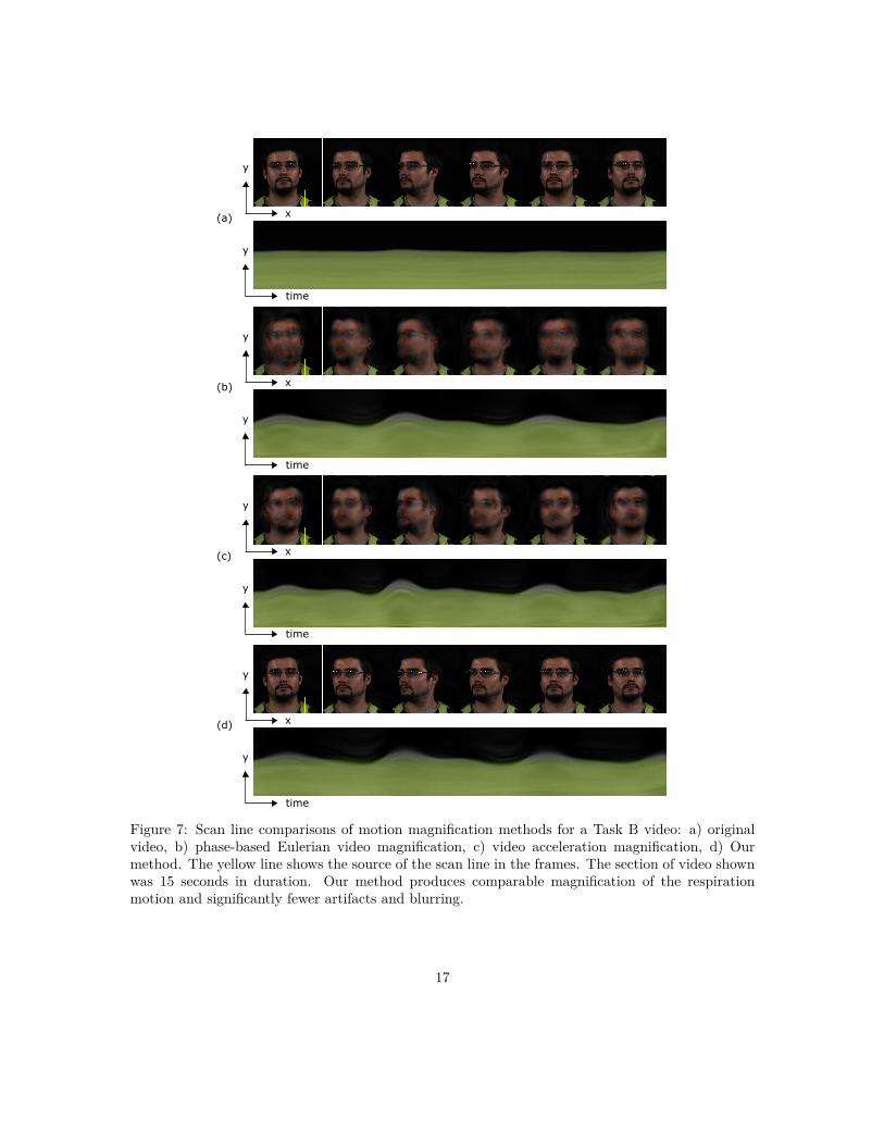
Figure 7: Scan line comparisons of motion magnification methods for a Task B video: a) originalvideo, b) phase-based Eulerian video magnification, c) video acceleration magnification, d) Ourmethod. The yellow line shows the source of the scan line in the frames. The section of video shownwas 15 seconds in duration. Our method produces comparable magnification of the respirationmotion and significantly fewer artifacts and blurring.

17

420.5Input

(a)

0 5 10 15 20 25 30

Time (second)

-30

-20

-10

0

10

Pha

se

(b)

0 5 10 15 20 25 30

Time (second)

-40

-20

0

20

40

Pha

se

(c)

0 5 10 15 20 25 30

Time (second)

-100

-50

0

50

100P

hase

0 5 10 15 20 25 30

Time (second)

-40

-20

0

20

40

60

Pha

se

(d)

Figure 8: Original and magnified traces of a pixel (the red dot) in the phase representation φ(r0, θ, t)of a Task C video along four orientations (a) θ = 0◦ (b) θ = 45◦ (c) θ = 90◦ (d) θ = 135◦. Magnifiedtraces using different step sizes γ are shown in different colors. The pixel exhibits a respirationmovement mainly in the vertical direction, so its magnified phase traces have the highest amplitudealong the θ = 90◦ orientation.

5.2 Motion MagnificationWe apply our method to the task of magnifying respiration motions. In this task the target variablefor training the CNN was the gold standard respiration signal measured via the chest strap. Giventhe subtle nature of the motions we found that a higher dimension input motion representation wasneeded than for the PPG magnification. As shown in Fig. 3, the motion representation was in 123pixels × 123 pixels × 4 orientations. The gradient ascent hyper-parameters N and γ were chosento be 20 and 3.6× 10−3 to produce moderate magnification effects.

Fig. 7 shows a qualitative comparison between our method and the baseline methods. Thehuman participant in the video rotated his head at a speed of 10 degrees/sec. A vertical scanline onhis shoulder was drawn along with time to show the respiration movement. In the input video, therespiration movement is very subtle. Both our method and the baseline methods greatly increased

18

Table 2: Video quality measured via Peak Signal-to-Noise Ratio (PSNR) and Structural Similarity(SSIM) for Task C videos magnified to different levels.

PSNR (dB) SSIMStep size 0.5γ γ 2γ 4γ 0.5γ γ 2γ 4γ

Pulse 43.2 42.6 41.6 39.9 0.987 0.987 0.986 0.986Respiration 42.0 41.4 40.6 39.6 0.982 0.979 0.974 0.965

its magnitude (Fig. 7 (b) (c) (d)). However, the baseline methods cannot clearly distinguish thephase variations caused by respiration and by head rotation, so it also amplified the head rotationand blurred the participant’s face. Our method is based on a better motion discriminator learnedvia the CNN so that the head motions are not amplified.

To show the intermediate phase variations and different magnification effects along different ori-entations, we drew the original and magnified traces of a pixel in the phase representation φ(r0, θ, t)(Fig. 8). Since the selected pixel is on the shoulder of the human participant, the respiration move-ment is mainly in the vertical direction. As a result, the amplified phase variations correspondingto breathing have the highest amplitude along θ = 90◦ (Fig. 8 (c)) and the lowest amplitude alongθ = 0◦ (Fig. 8 (a)). We also changed the chosen step size γ to its multiples (0.5γ, 2γ and 4γ) withthe number of iterations N unaltered, and visualized the resulting phase traces in Fig. 8. The figuresuggests that the magnification level always increases along with the step size.

The same quantitative metrics as those for color magnification were computed and shown inTable 1. They also generally follow the same pattern as in the color magnification analysis: Thevideo quality of the baseline methods is impacted by the level of head motions, while our methodis considerably more robust. There is no significant difference between our participant-dependentresults and participant-independent results.

0 5 10 15

Number of iterations

0

500

1000

1500

2000

2500

3000

Loss

0 5 10 15

Number of iterations step size ( )

0

200

400

600

800

1000

1200

Loss

0.5

24

(a) (b)

Figure 9: Learning curves: (a) The change of the CNN loss with different numbers of iterations Nand different step sizes γ. (b) The change of the CNN loss with different products of N and γ.

5.3 Magnification FactorsThe magnification factor of our algorithm is controlled by two hyper-parameters, the number ofiterations N and the step size γ. In Fig. 6 and Fig. 8, we chose the same N and tuned γ to

19

be different multiples. The resulting magnification levels were always higher when γ was longer.However, there is a trade-off in the selection of γ, as a higher magnification factor also introducesmore artifacts. Table 2 shows the average video quality metrics PSNR and SSIM for our outputvideos on an exemplary task (Task C) with different choices of γ. For both the pulse and respirationmagnification tasks, the video quality decreases to different extents with the increase of γ. Giventhat artifacts considerably reduce the PSNR and SSIM metrics (as shown in Table 1), the fact thatthe values do not change dramatically with γ shows that few artifacts are introduced with increasingmagnification.

To quantitatively analyze the effects of N and γ on the magnification factor, we drew exemplarylearning curves for one of our videos in Fig. 9 (a) with different choices of parameters. The curvesshow the changes of our CNN loss, the L2 norm of the differential motion signal, which is a goodestimate of the target motion magnitude. According to the learning curves, both N and γ positivelycorrelate with the motion magnitude, and the relationship between N and the motion magnitudeis semi-linear. However, a longer step size with fewer iterations is not equivalent to a shorter stepwith more iterations. In Fig. 9 (b), we show how the loss changes along with the product of N andγ, which suggests that relatively small step sizes and more iterations can increase the magnificationfactor more efficiently.

(a)

(b)

0 5 10 15 20 25 30

Time (second)

0

0.2

0.4

0.6

0.8

L1 n

orm

0 0.2 0.4 0.6 0.8

L1 norm

0

100

200

300

400

Num

ber

of fr

ames

0 5 10 15 20 25 30

Time (second)

0

0.02

0.04

0.06

0.08

0.1

L1 n

orm

0 0.01 0.02 0.03 0.04 0.05

L1 norm

0

500

1000

1500

Num

ber

of fr

ames

*

Figure 10: (a) Time series and histograms of the L1 norms of the input motion representation X1for a 30-second video. (b) Time series and histograms of the L1 norms of the motion gradient∇‖y(X1|θ)‖2 for the same video.

5.4 Gradient Ascent MechanismsCompared with traditional gradient ascent, we added two new mechanisms to adapt the approach tothe task of video magnification: L1 normalization and sign correction. Here we show experimentalresults to support the necessity of these mechanisms.

20

-1

-0.5

0

0.5

1

(a) (b) (c)

Figure 11: Pixel-wise correlation coefficients between the input and magnified motion representationsin the respiration magnification task, with the sign correction mechanism (b) and without the signcorrection mechanism (c).

The goal of applying L1 normalization is to make sure every frame in a video is magnified tothe same level. To achieve this goal, the gradient ∇‖y(Xn|θ)‖2 in (1) needs to be approximatelyproportional to the motion representation Xn. However, it was not the case without L1 normaliza-tion. Fig. 10 shows the time series and histograms of the L1 norms of X1 and ∇‖y(X1|θ)‖2 for a30-second video. It is obvious that the distribution of the motion representation is Gaussian whilethe distribution of the gradient is highly skewed. To correct the distribution of the gradient to matchthe motion representation, it needs to be L1 normalized.

In Fig. 11, we show the pixel-wise correlation coefficients between the input and the magnifiedmotion representations in the respiration magnification task, with and without the sign correctionmechanism. When there is no sign correction, the correlation coefficients have both positive andnegative values (Fig. 11 (b)). As introduced in Section 3.1, the negative values appear because thetarget motion could be amplified with its direction reversed. In the example in Fig. 11 (b), most ofthe negative values happen on the background, which are negligible as the background has nearly nomotion to amplify, but some of them are on the human body, which will cause the output video tobe blurry on magnification. After sign correction is applied, all the correlation coefficients becomepositive (Fig. 11 (c)).

6 ConclusionsRevealing subtle signals in our everyday world is important for helping us understand the processesthat cause them. We present a novel single deep neural framework for video magnification that isrobust to large rigid motions. Our method leverages a CNN architecture that enables magnificationof a specific source signal even if it overlaps with other motion sources in the frequency domain.We present several methodological innovations in order to achieve our results, including adding L1normalization and sign correction to the gradient ascent method.

Pulse and respiration magnification are good exemplar tasks for video magnification as thesephysiological phenomena cause both subtle color and motion variations that are invisible to theunaided eye. Our qualitative evaluation illustrates how the PPG color changes and respirationmotions can be clearly magnified. Comparisons with baseline methods show that our proposedarchitecture dramatically reduces artifacts when there are other rotational head motions present in

21

the videos.In a systematic quantitative evaluation our method improves the PSNR and SSIM metrics across

tasks with different levels of rigid motion. By magnifying a specific source signal we are able tomaintain the quality of the magnified videos to a greater extent.

References[1] Guha Balakrishnan, Fredo Durand, and John Guttag. “Detecting pulse from head motions in

video”. In: Proceedings of the IEEE Computer Society Conference on Computer Vision andPattern Recognition (2013), pp. 3430–3437. issn: 10636919.

[2] Pak-Hei Chan et al. “Diagnostic performance of a smartphone-based photoplethysmographicapplication for atrial fibrillation screening in a primary care setting”. In: Journal of the Amer-ican Heart Association 5.7 (2016), e003428.

[3] Weixuan Chen and Daniel McDuff. “DeepPhys: Video-Based Physiological Measurement UsingConvolutional Attention Networks”. In: arXiv preprint arXiv:1805.07888 (2018).

[4] Mohamed Elgharib et al. “Video magnification in presence of large motions”. In: Proceedingsof the IEEE Conference on Computer Vision and Pattern Recognition. 2015, pp. 4119–4127.

[5] Dumitru Erhan et al. “Visualizing higher-layer features of a deep network”. In: University ofMontreal 1341.3 (2009), p. 1.

[6] Justin R Estepp, Ethan B Blackford, and Christopher M Meier. “Recovering pulse rate duringmotion artifact with a multi-imager array for non-contact imaging photoplethysmography”. In:2014 IEEE International Conference on Systems, Man and Cybernetics (SMC). IEEE. 2014,pp. 1462–1469.

[7] Thomas B Fitzpatrick. “The validity and practicality of sun-reactive skin types I through VI”.In: Archives of dermatology 124.6 (1988), pp. 869–871.

[8] Martin Fuchs et al. “Real-time temporal shaping of high-speed video streams”. In: Computers& Graphics 34.5 (2010), pp. 575–584.

[9] Temujin Gautama and MA Van Hulle. “A phase-based approach to the estimation of theoptical flow field using spatial filtering”. In: IEEE Transactions on Neural Networks 13.5(2002), pp. 1127–1136.

[10] Gerard de Haan and Vincent Jeanne. “Robust pulse rate from chrominance-based rPPG”. In:IEEE Transactions on Biomedical Engineering 60.10 (2013), pp. 2878–2886.

[11] Gerard de Haan and Arno van Leest. “Improved motion robustness of remote-PPG by usingthe blood volume pulse signature”. In: Physiological measurement 35.9 (2014), p. 1913.

[12] Rik Janssen et al. “Video-based respiration monitoring with automatic region of interest de-tection”. In: Physiological Measurement 37.1 (2016), pp. 100–114. issn: 0967-3334.

[13] Gunter Klambauer et al. “Self-normalizing neural networks”. In: Advances in Neural Informa-tion Processing Systems. 2017, pp. 972–981.

[14] Antony Lam and Yoshinori Kuno. “Robust heart rate measurement from video using selectrandom patches”. In: Proceedings of the IEEE International Conference on Computer Vision.2015, pp. 3640–3648.

22

[15] Ce Liu et al. “Motion magnification”. In: ACM transactions on graphics (TOG) 24.3 (2005),pp. 519–526.

[16] Daniel McDuff. “Deep Super Resolution for Recovering Physiological Information from Videos.”In: Proceedings of the IEEE Conference on Computer Vision and Pattern Recognition Work-shops. 2018.

[17] Daniel McDuff, Sarah Gontarek, and Rosalind Picard. “Improvements in Remote Cardio-Pulmonary Measurement Using a Five Band Digital Camera.” In: IEEE Transactions onBiomedical Engineering 61.10 (2014), pp. 2593–2601.

[18] Daniel McDuff et al. “A survey of remote optical photoplethysmographic imaging methods”.In: 2015 37th Annual International Conference of the IEEE Engineering in Medicine andBiology Society (EMBC). IEEE. 2015, pp. 6398–6404.

[19] Hamed Monkaresi, Rafael A Calvo, and Hong Yan. “A machine learning approach to improvecontactless heart rate monitoring using a webcam”. In: IEEE journal of biomedical and healthinformatics 18.4 (2014), pp. 1153–1160.

[20] Alexander Mordvintsev, Christopher Olah, and Mike Tyka. “Deepdream-a code example forvisualizing neural networks”. In: Google Res 2 (2015).

[21] Masahiro Mori. “The uncanny valley”. In: Energy 7.4 (1970), pp. 33–35.[22] Tae-Hyun Oh et al. “Learning-based Video Motion Magnification”. In: arXiv preprint arXiv:1804.02684

(2018).[23] Chris Olah, Alexander Mordvintsev, and Ludwig Schubert. “Feature visualization”. In: Distill

(2017).[24] Ahmed Osman, Jay Turcot, and Rana El Kaliouby. “Supervised learning approach to remote

heart rate estimation from facial videos”. In: 2015 11th IEEE International Conference andWorkshops on Automatic Face and Gesture Recognition (FG). Vol. 1. IEEE. 2015, pp. 1–6.

[25] Ming-Zher Poh, Daniel J McDuff, and Rosalind W Picard. “Advancements in noncontact, mul-tiparameter physiological measurements using a webcam”. In: IEEE Transactions on Biomed-ical Engineering 58.1 (2011), pp. 7–11.

[26] Ming-Zher Poh, Daniel J McDuff, and Rosalind W Picard. “Non-contact, automated cardiacpulse measurements using video imaging and blind source separation”. In: Optics Express 18.10(2010), pp. 10762–10774.

[27] Javier Portilla and Eero P Simoncelli. “A Parametric Texture Model Based on Joint Statisticsof Complex Wavelet Coefficients”. In: International Journal of Computer Vision 40.1 (2000),pp. 49–71.

[28] E.P. Simoncelli et al. “Shiftable multiscale transforms”. In: IEEE Transactions on InformationTheory 38.2 (Mar. 1992), pp. 587–607. issn: 0018-9448.

[29] Karen Simonyan, Andrea Vedaldi, and Andrew Zisserman. “Deep inside convolutional net-works: Visualising image classification models and saliency maps”. In: arXiv preprint arXiv:1312.6034(2013).

[30] Supasorn Suwajanakorn, Steven M Seitz, and Ira Kemelmacher-Shlizerman. “Synthesizingobama: learning lip sync from audio”. In: ACM Transactions on Graphics (TOG) 36.4 (2017),p. 95.

23

[31] Chihiro Takano and Yuji Ohta. “Heart rate measurement based on a time-lapse image”. In:Medical engineering & physics 29.8 (2007), pp. 853–857.

[32] K.S. Tan et al. “Real-time vision based respiration monitoring system”. In: 7th InternationalSymposium on Communication Systems Networks and Digital Signal Processing (CSNDSP)(2010), pp. 770–774. issn: 00189294.

[33] L Tarassenko et al. “Non-contact video-based vital sign monitoring using ambient light andauto-regressive models”. In: Physiological Measurement 35.5 (2014), pp. 807–831. issn: 0967-3334.

[34] Sergey Tulyakov, Xavier Alameda-Pineda, and Elisa Ricci. “Self-adaptive matrix completionfor heart rate estimation from face videos under realistic conditions”. In: Proc. ComputerVision Pattern Recognition (2016), pp. 2396–2404. issn: 10636919.

[35] Wim Verkruysse, Lars O Svaasand, and J Stuart Nelson. “Remote plethysmographic imagingusing ambient light”. In: Optics express 16.26 (2008), pp. 21434–21445.

[36] Neal Wadhwa et al. “Phase-based video motion processing”. In: ACM Transactions on Graphics(TOG) 32.4 (2013), p. 80.

[37] Neal Wadhwa et al. “Riesz pyramids for fast phase-based video magnification”. In: 2014 IEEEInternational Conference on Computational Photography (ICCP). IEEE. 2014, pp. 1–10.

[38] Jue Wang et al. “The cartoon animation filter”. In: ACM Transactions on Graphics (TOG).Vol. 25. 3. ACM. 2006, pp. 1169–1173.

[39] Wenjin Wang, Sander Stuijk, and Gerard de Haan. “Exploiting Spatial Redundancy of ImageSensor for Motion Robust rPPG.” In: IEEE Transactions on Biomedical Engineering 62.2(2015), pp. 415–425.

[40] Wenjin Wang et al. “Algorithmic Principles of Remote-PPG”. In: IEEE Transactions onBiomedical Engineering PP.99 (2016), pp. 1–12. issn: 15582531.

[41] Hao-Yu Wu et al. Eulerian video magnification for revealing subtle changes in the world. 2012.[42] Hao-Yu Wu et al. “Eulerian video magnification for revealing subtle changes in the world.” In:

ACM Trans. Graph. 31.4 (2012), p. 65.[43] Shuchang Xu, Lingyun Sun, and Gustavo Kunde Rohde. “Robust efficient estimation of heart

rate pulse from video”. In: Biomedical Optics Express 5.4 (2014), p. 1124. issn: 2156-7085.[44] Yichao Zhang, Silvia L. Pintea, and Jan C. Van Gemert. “Video acceleration magnification”.

In: Proceedings - 30th IEEE Conference on Computer Vision and Pattern Recognition (2017),pp. 502–510.

24