arX

iv:1

401.

0546

v1 [

cs.N

E]

2 Ja

n 20

141

Low-Complexity Particle Swarm Optimization

for Time-Critical ApplicationsMuhammad S. Sohail, Muhammad O. Bin Saeed,Member, Syed Z. Rizvi,Student Member

Mobien Shoaib,Memberand Asrar U. H. Sheikh,Fellow

Abstract

Particle swam optimization (PSO) is a popular stochastic optimization method that has found wide applications

in diverse fields. However, PSO suffers from high computational complexity and slow convergence speed. High

computational complexity hinders its use in applications that have limited power resources while slow convergence

speed makes it unsuitable for time critical applications. In this paper, we propose two techniques to overcome these

limitations. The first technique reduces the computationalcomplexity of PSO while the second technique speeds up

its convergence. These techniques can be applied, either separately or in conjunction, to any existing PSO variant.

The proposed techniques are robust to the number of dimensions of the optimization problem. Simulation results are

presented for the proposed techniques applied to the standard PSO as well as to several PSO variants. The results show

that the use of both these techniques in conjunction resultsin a reduction in the number of computations required as

well as faster convergence speed while maintaining an acceptable error performance for time-critical applications.

Index Terms

Particle swarm optimization (PSO), low complexity, fast convergence, swarm intelligence, optimization.

I. I NTRODUCTION

Since its introduction, the particle swarm optimization (PSO) algorithm [1]-[2] has attracted a lot of attention

due to its ability to effectively solve a large number of problems in diverse fields. Optimization problems generally

involve maximization or minimization of an objective function, often subject to multiple constraints. The notion of

using a swarm of agents that help each other in a directed search to find an optimal solution to a problem has been

received with much enthusiasm by the research community globally, as it brought a much-needed enrichment to

the existing computational arsenal.

The improvements and advancements in the PSO algorithm resulted in algorithms that are used in numerous

applications. For example, the authors in [3] used PSO and ant colony algorithms to devise an adaptive routing

algorithm for a mobile ad hoc network. The work in [4] used thePSO algorithm to propose a multihop virtual

MIMO communication protocol with a cross-layer design to improve the performance and life of a wireless sensor

network. PSO-based adaptive channel equalization was proposed in [5]-[7] while [8]-[9] used PSO for multiuser

detection in CDMA systems. The works in [10]-[11] used the PSO algorithm for radar design. PSO was used for

DRAFT

2

MIMO receivers [12], adaptive beamforming [13] and economic dispatch problems [14]-[19]. PSO also found use in

several antenna applications [20] such as the design of phased arrays [21]-[22] and broadband antenna design [23].

Other applications in which the PSO algorithm was successfully implemented include controller design [24]-[26],

power systems [27], biometrics [28], distribution networks [29], electromagnetics [30], robotics [31], gaming [32]

and data clustering [33], [34], [35]. A detailed survey of PSO applications can be found in [36]-[37].

Despite the popularity of PSO, it suffers from the issues of high computational complexity and considerable

convergence time. This hinders its use in applications thatrequire fast convergence or have power/computational

constraints.

In this work, we propose two new techniques aimed at reducingcomputational complexity as well as improving the

speed of convergence of the PSO algorithm. An event-triggering-based approach reduces the number of computations

for an acceptable degradation in performance. This is followed by a dimension-wise cost function evaluation

technique that increases the speed of convergence as well asimproving overall performance. The techniques can

be applied to any existing PSO variant either exclusively, or in conjunction.

The paper is arranged as follows. In Section II, we take a lookat some of the important variants of PSO

and assess in detail the merits and costs of each algorithm. In Section III we present an event-triggering-based

approach to reduce the computational complexity of the particle swarm search algorithm. Section IV takes a look

at the dimension-wise search for particle position, aimed at obtaining faster convergence towards optimal solutions.

Section V discusses how the two approaches can be combined for optimum results. Section VI discusses the

experimental results while Section VII presents the conclusion.

II. T HE PARTICLE SWARM OPTIMIZER AND ITS VARIANTS

We start with a brief recap of the working of the PSO algorithmand then discuss some of its variants. The PSO

algorithm is a population based optimization method that imitates swarm behavior observed in a herd of animals

or a school of fish. The swarm consists of particles representing the set of optimization parameters. Each particle

searches for a potential solution in a multi-dimensional search space. The aim of the algorithm is to converge to

an optimum value for each parameter. The estimate for each particle is tested using a fitness function. The fitness

function when evaluated, gives a fitness value that defines the ”goodness” of the estimate. Each particle has two

state variables, namely “particle position”x(i) and “particle velocity”v(i) , wherei denotes iteration index. The

fitness of an individual particle is measured by evaluating the cost function for that particle. Every particle combines

its own best attained solution with the best solution of the whole swarm to adapt its search pattern. For a swarm

of N particles traversing aD-dimensional space, the velocity and position of each particle are updated as [1]

vdk (i+ 1) = vdk (i) + c1 · r1,k(i) ·(

pdk − xdk (i)

)

+ c2 · r2,k(i) ·(

gd − xdk (i)

)

, (1)

xdk (i+ 1) = xd

k (i) + vdk (i+ 1) , (2)

DRAFT

3

whered = 1, · · · , D denotes the particle’s dimension index andk = 1, · · · , N is the particle index. The constants

c1 andc2 are called the cognitive and social parameters, and are responsible for defining a particle’s affinity towards

its own best and the global best solutions, respectively. The variablesvdk andxdk are the velocity and position of

the k-th particle corresponding to itsd-th dimension whilepdk andgd are the particle’s local best and the swarm’s

global best positions for thed-th dimension respectively. The variablesr1,k and r2,k are drawn from a uniform

random distribution[0, 1] and are the source of randomness in the search behavior of theswarm.

Of the earliest variants to the original algorithm, Eberhart and Shi proposed an inertia-weight model [38], which

multiplies the velocity of the current iteration with a factor known as the inertia weight

vdk (i+ 1) = w · vdk (i) + c1 · r1,k(i) ·(

pdk − xdk (i)

)

+ c2 · r2,k(i) ·(

gd − xdk (i)

)

. (3)

The inertia weight, w ∈ [0, 1], ensures convergence and controls the momentum of the particle. If w is

too small, very little momentum is preserved from the previous iteration and thus quick changes of direction are

possible. Ifw = 0, the particle moves without knowledge of the past velocity profile. On the other hand, a very

high value of inertia weight means that the particles can hardly change their direction, which translates into more

exploration and slow convergence. Maurice and Clerc later introduced a constriction-factor [39] to constrict the

velocity by multiplying it with this factor before updatingthe position of the particle. The constriction factor model

has the same effect as the inertia weight model, except for the fact that it scales the contributions from both the

local and global best solutions, thus limiting the search space. Low values facilitate rapid convergence but at the

cost of smaller exploration space and vice versa.

This initial model of the PSO optimizer is very efficient in converging to near-optimal solutions for uni-modal

problems, i.e. problems that do not have local minima. The algorithm therefore converges quickly to optimal or near-

optimal solution. However, when the problem is multi-modal, then too fast a convergence often leads to entrapment

of the algorithm in a local optimum. The algorithm must explore different solution areas in such a case before

converging in order to avoid getting stuck in a sub-optimal region.

Shortly after the first few PSO variants appeared in literature, significant progress was made towards solving

multi-modal problems with the development of neighborhoodtopologies. It was suggested that instead of each

particle being connected to the whole swarm, it should be connected to a small neighborhood of particles and if

each neighborhood had its own global best solution, then different solution areas of the swarm would be explored,

thus avoiding entrapment in local minima. Thus, in the localversion of PSO (LPSO), the velocity of each particle is

adjusted according to its personal best and the best performance achieved so far within its neighborhood. Kennedy

and Mendes have discussed the effects of various populationtopologies on the PSO algorithm in [40]. To test

this, benchmark problems were solved using different topologies. The authors stated that information moves fastest

between connected pairs of particles, and is slowed down by the presence of intermediate particles. They further

concluded that the conventional PSO topology known as “global best topology” facilitates the most immediate

communication possible. However, on complex multi-modal problems, this is not necessarily desirable and the

DRAFT

4

population will fail to explore outside of locally optimal regions.

The ring topology known as “local best” is the slowest and most indirect communication pattern and a solution

found by a particle moves very slowly around the ring. However, this ensures proper exploration which is desirable

in multi-modal complex problems. One variant, proposed by Peram et. al., is known as fitness-distance-ratio (FDR)

PSO, with near neighbor interactions [41]. The FDR-PSO selects one other particle having higher fitness value near

the particle being updated, in the velocity updating equation. Other variants which used multi-swarm [42] or sub-

population [43] are also generally included under LPSOs since the sub-groups are treated as special neighborhood

structures.

Similar conclusions were derived by Liang and Suganthan whoproposed a dynamic multi-swarm particle swarm

(DMS-PSO) [44]. It can be said that in topology-based LPSO algorithms, a trade-off between the speed of exploration

and depth of exploration hinges upon the “granularity” of the neighborhood used. Liang and Suganthan showed

with simulations that on uni-modal benchmark functions like the sphere function, all algorithms perform almost

equally well.

Mendes et al. proposed a fully informed particle swarm (FIPS) [45], in which all the neighborhood is a source of

influence rather than just one particle. Chatterjee and Siarry [46] presented a modified version of the PSO algorithm

where they proposed a nonlinear variation of inertia weightalong with a particle’s old velocity in order to speed

up the convergence as well as fine tune the search in the multi-dimensional space. Hu and Eberhart [47] used a

dynamic neighborhood where closest particles in the searchspace are selected to be a particle’s new neighborhood

in each generation. Parsopoulos and Vrahatis combined the global version and local version together and constructed

a unified particle swarm optimizer UPSO [48].

There have been several efforts in investigating hybridization by combining PSO with other search techniques

to improve the performance of the PSO. Evolutionary operators such as selection, crossover, and mutation were

used in PSO to keep the best particles [49], to increase the diversity of the population, and avoid entrapment in

a local minimum [43]. The use of mutation operators was explored to mutate parameters like inertia weight [50].

Relocation of particles was used in [51]. In [52] collision-avoiding mechanisms were introduced to prevent particles

from moving too close to each other. This, according to the authors, helps maintain the diversity in the swarm and

helps to escape local optima. In [53], deflection, stretching, and repulsion techniques were used to find maximum

possible minima by preventing particles from moving to a previously discovered minimal region. An orthogonal

learning technique combined with orthogonal experimentaldesign were used to enhance performance in orthogonal

PSO (OPSO) [54] and orthogonal learning PSO (OLPSO) [55], although at the cost of very high computational

complexity.

A cooperative particle swarm optimizer (CPSO) was proposedin [56]. The CPSO uses one-dimensional swarms

and searches each of them separately, so as to avoid the “curse of dimensionality” that plagues most stochastic

optimization algorithms including PSO and genetic algorithms. These separate searches are then integrated together

by a global swarm. This results in significant improvement over the performance of the standard PSO algorithm

when solving multimodal problems albeit at a much higher computational cost.

DRAFT

5

Ratnaweera et al. suggested a self-organizing hierarchical PSO (HPSO) algorithm with time-varying acceleration

coefficients [57]. The inertia weight term is removed with the idea that only the acceleration coefficients should

guide the movement of the particle towards the optimum solution. Both the acceleration coefficients vary linearly

with time. If the velocity goes to zero at some point, the particle is re-initialized using a predefined starting velocity.

Due to this self-organizing and self-restarting property,the HPSO algorithm achieves outstanding results.

The comprehensive learning PSO (CLPSO) algorithm of [58] provides the best performance-complexity trade-off

among all existing PSO variants. It divides the unknown estimate into sub-vectors. A particle chooses two random

neighbor particles for each sub-vector, and chooses a sub-vector as an exemplar based on the best fitness value

for that particular sub-vector. The combined result of all sub-vectors gives the overall best vector, which is then

used to perform the update. If the particle stops improving for a certain number of iterations, then the neighbor

particles for the sub-vectors are changed. The success of this technique may be attributed to its exploitation of the

“best information” profile (or trend) of all other particlesin updating the velocity equation, as this rich historical

information will help improve the predictive power of the velocity equation. The authors claimed that although

their variant did not perform well on uni-modal problems, itoutdid most variants on multi-modal problems. When

solving real-world problems, one usually does not know the shape of the fitness landscape. Hence, the authors

concluded that, in such cases, it is advisable to use an algorithm that performs well on multimodal problems.

However, it is our humble opinion that the algorithms presented in literature, despite their accurate performances,

are still slow in convergence and far computationally complex for time-critical and power-limited applications.

Keeping in mind all of these very important works, our aim in this paper is to propose an algorithm that emphasizes

on quick convergence and low-complexity while still maintaining significant accuracy acceptable to real world

problems.

III. E VENT-TRIGGERING IN PARTICLE SWARM OPTIMIZATION

The first technique is aimed at reducing the number of computations of the PSO algorithm. We begin by first

analyzing the complexity of the standard PSO algorithm and then we derive a motivation for our approach.

A. Complexity of the Standard PSO Algorithm

The number of computations required for a complete run of thePSO algorithm are the sum of the computations

required to calculate the cost of a candidate solution (based on current position of the particles) and the computations

required to update each particle’s position (2) and velocity (3). Both of these are directly proportional to the number

of iterations.

The computational complexity of evaluating the cost function depends on the particular cost function under

consideration. For example, the sphere function (see TableI) requiresD multiplications per particle per iteration,

resulting in a total ofDN multiplications for cost function evaluation per iteration. Similarly, the Rosenbrock

function (see Table I) requires4DN multiplications. These computations need to be performed at every iteration

for all PSO variants and cannot be reduced.

DRAFT

6

For the second set of computations (i.e., the ones required for the update equations), the standard PSO algorithm

requires5DN multiplications per iteration. This number is5 times the number of multiplications required for the

sphere function and1.25 times that required by the Rosenbrock function. This shows that the cost associated with

the update equations makes a significant contribution to thetotal computational cost of the PSO algorithm.

B. Motivation

It is observed that many PSO variants tend to achieve accuracy levels that are not required in most practical

applications. For example, OLPSO and CPSO are able to give solutions that have an error range of about1e−200 or

1e−300 [55], [56]. Both these algorithms achieve this high degree of accuracy at the cost of significant computational

overhead. We also note that in many applications, such high level of accuracy is generally not required as i) they

operate in noisy environment and have a bound on accuracy dueto the noise floor ii) a solution within a certain error

margin would be considered sufficiently accurate and a lowererror margin would result in minimal improvement

in system performance.

Such a scenario frequently occurs in devices that have limited computational power (where finite machine precision

would impose a limit on the level of accuracy that can be achieved) or limited power budget (for instance battery

operated devices where it is desirable to minimize power consumption by performing only the necessary required

computations). Similarly, many scenarios only require theestimate or solution to be accurate to a particular degree

and a more accurate solution will not necessarily yield performance gain. For example, if the problem is to find

the optimal weights of a neural network or optimal filter weights for an estimation problem or optimal distance

calculations, then in engineering terms, a solution that has an accuracy of1e−5 might be as good as one that has

an accuracy of1e−30.

Based on the analysis in the previous subsection, we computethe number of multiplications that would typically

be needed by the standard PSO in a given scenario. For a typical swarm of40 particles optimizing a problem with

say30 dimensions, a total of5 × 40 × 30 = 6, 000 multiplications need to be performed per iteration for the

update equations (2) and (3). Even if the PSO algorithm runs for only 100 iterations, then6, 000× 100 = 600, 000

multiplications need to be performed just for the update equations. Note that this number does not include the

number of multiplications required for calculating the cost function for each particle at each iteration.

With this in view, we propose reducing the number of computations at the cost of acceptable performance

degradation (we show in Section VI that using our two proposed techniques, the performance degradation is

negligible for all practical purposes). To this end, we propose an event-triggering-based approach described below

in detail.

C. The Event-Triggering Approach

We rewrite (3) as

vdk (i+ 1) = w · vdk (i) + α(i) + β(i) (4)

DRAFT

7

whereα(i) andβ(i) represent the cognitive and social terms respectively. We note that the cognitive term consists

of a constantc1, random variable (drawn from a uniform distribution over the interval [0, 1]) and the distance

between the particle’s current position and the local best position. This distance acts like a scaling factor that sets

an upper limit on the maximum value of the cognitive term. Thedistance between thed-th dimension of the global

best and the particle’s current position has a similar role for the social term.

We define the particle’s local distance for itsd-th dimension as the absolute difference between the particle’s

current position and its local best position. The particle’s global distance is defined in a similar fashion as the

absolute difference between the particle’s current position and its global best position, i.e.,

local distance =∣

∣pdk − xdk

∣

∣ (5)

global distance =∣

∣gd − xdk

∣

∣ . (6)

If the local distance is smaller than a certain preset threshold, denoted byγ, then the cognitive term in (4) is set

to zero, i.e., it is not involved in the update process. The value of γ is usually small. Mathematically

α(i) =

c1 · r1,k(i) ·(

pdk − xdk (i)

)∣

∣pdk − xdk (i)

∣

∣ ≥ γ

0∣

∣pdk − xdk (i)

∣

∣ < γ

(7)

The idea here is that if thed-th dimension of the particle is very close to thed-th dimension of its local best,

the contribution of the cognitive term of (4) will be very small, and hence can be ignored with negligible effect on

the value ofvdk (i+ 1). The velocity of the particle for thed-th dimension would still be updated on the basis of

its inertia weight term and the social term,β.

Similarly, if thed-th dimension of the particle is very close to thed-th dimension of the global best of the swarm

then the contribution of the social term in the update of (4) would be negligible and can be ignored. That is

β(i) =

c2 · r2,k(i) ·(

gd − xdk (i)

) ∣

∣gd − xdk (i)

∣

∣ ≥ γ

0∣

∣gd − xdk (i)

∣

∣ < γ

(8)

Thus, the cognitive and social terms of the update equation for the d-th dimension will not be calculated if

the particle’s current position is withinγ distance of its local best position and the swarm’s global best position,

respectively. Note that these terms can be ignored in such a case owing to their negligible contributions to the

update equation for this particular dimension. This can be viewed as an event-triggering approach. The particle’s

velocity in thed-th dimension is still updated due to the inertia weight term. Note that the proposed technique does

not hinder the exploration by the particle in other dimensions. The technique merely avoids calculating those terms

that would have negligible contribution to the velocity update (3). Although we have considered the same value of

γ for all D dimensions, different values can be used for each dimensionif the scenario calls for different margin

of errors for various parameters (dimensions) of the problem.

DRAFT

8

IV. EXPLOITING SEPARABILITY AND DIMENSION-WISE SEARCH

In this section, we present the second proposed technique which aims to speed up the convergence.

A. Motivation

It is known that PSO suffers from the so called “two steps forward, one step backward” phenomenon [56]

as explained by the following example. Consider a3-dimensional sphere function with cost given asf(x) =

x21 + x2

2 + x23. Let thek-th particle’s local best position bepk = [7, 5,−1] with cost75 and the position after the

velocity update bexk = [6, 4,−3] with cost61. This would cause thek-th particle to update its local best position

to pk = [6, 4,−3] even though the third dimension of the old local best vector was better than the third dimension

of the new local best vector. This happens because the increased cost of the third dimension ofxk is compensated

by the gains of the first and the second dimensions; resultingin an overall lower cost ofxk. Although the overall

cost has reduced, the third dimension is now further away from its optimal position. This motivates us to find

an update rule that can avoid this “two steps forward, one step backward” phenomenon and somehow retain the

“good” dimension during particle updates.

Another motivation for this approach is the simple fact thatit is easier to deal with one dimension at a time; akin

to the divide and conquer strategy. For problems with separable cost functions (discussed in the next subsection),

each dimension can be optimized independently of the others. Although not true for every problem, it turns out

that many important real-life problems have separable costfunctions. This motivates us to investigate if separability

can be exploited to aid the PSO algorithm for problems with separable cost functions.

Many time-critical applications require fast convergence. As such, the third motivation for this approach is to

find a way to speed up the convergence of the PSO algorithm.

B. Separable Cost Functions

The cost functions in which each term depends on only a singledimension are termed as separable cost functions

such as Sphere, Rastrigin and Sum-of-Powers functions. Thus, aD-dimensional Sphere function, given byf(x) =

x21 + x2

2 + · · · + x2D, can be separated intoD terms, with thed-th term beingx2

d, such that the summation of all

D terms gives the vector-cost of the sphere function. Some examples of applications with separable cost functions

include adaptive routing in mobile ad hoc networks [3], adaptive channel equalization [5]-[7], multiuser detection

[8], [9], adaptive beamforming [12], [13], economic dispatch [14]-[19], biometrics [28], robotics [31], and data

clustering [34], [35].

C. Behavior of Standard PSO Algorithm

In addition to the “two steps forward, one step backward” phenomenon, the characteristic behavior of the PSO

algorithm also manifests itself in another way. Consider a standard PSO algorithm optimizing aD-dimensional

problem. The update mechanism of the standard PSO updates the particle position vectors according to (2). The

new particle position of thek-th particle,xk, is compared to the particles local best,pk. If the former has lower

DRAFT

9

cost,xk becomes the new value of particle’s local best while if the cost of the latter is less than that of the former,

the current local best is retained. Similarly, the local best solution with the least cost among all particles is chosen

as the global best solution.

These comparisons are based on the aggregate total cost calculations and are oblivious to the rich information

contained by the particles on the single-dimension level. The cost associated with a particle might be lower for

a solution p1 as compared to solution p2 and yet on the single-dimensional level, we may find that p2 has some

values for certain dimensions that are more fit than their counter parts in solution p1. This happens because the

normal update rule seeks to minimize the overall cost of the particle position vector and ignores the picture on the

single-dimensional level. The idea is best explained by thefollowing example.

We consider a3-dimensional sphere function with cost given asf(x) = x21 + x2

2 + x23. Let thek-th particle’s

local best position bepk = [0, 7, 3], its position after the velocity update bexk = [8, 4,−1] and the global best

position beg = [−4, 2, 6]. The corresponding costs are58, 81 and56. As the updated position of the particle has

a higher cost,81, than the particle’s local best,58, the conventional total cost based update rule would retainthe

current local best. Also, the current local best vector of the k-th particle has a higher cost,58, than the global best

vector,56, and thus, it will not effect the update of the global best vector. Thus, the particle will not learn anything

new fromxk in this generation.

However, if we observe carefully, bothpk andxk contain useful information. The best vector that can be generated

by combining components ofpk andxk is [0, 4,−1] which has a cost of17. The cost of this new vector is lower

than the current particle best and hence it would become the new particle best. For simplicity, even if we neglect

the particle best of all other particles and compare the global best only with thek-th particle’s updated local best,

we see that the optimum vector that can be formed by picking individual components of these solutions is[0, 2,−1]

which yields a minimum cost of5. Thus the standard PSO fails to use this rich information contained in individual

dimensions.

D. The Dimension-wise Approach

One strategy to find the optimal local best can be to run a bruteforce exhaustive search to test all possible

vectors that can be formed by combining the individual vector components ofpk andxk. Similarly, the strategy for

the global best can be to run a similar exhaustive search overall local bests to find the global best vector. While

this may be possible for the scenario when both the problem dimension,D, and the swarm size,K, are small,

the strategy is utterly unfeasible for scenarios with largevalues ofD andK. It is worth mentioning here that the

typical swarm size (K = 40) is much too large to entertain the exhaustive search strategy. Interestingly, it turns out

that if we focus on the class of problems that have separable cost functions, the optimum local/global best vector

can be found at the same computational complexity as the standard PSO.

The dimension-wise cost evaluation strategy works as follows: Divide the swarm intoD 1-dimensional swarms.

Each swarm optimizes a single dimension. Run the regular PSOupdate equations (2) and (3). Calculate the cost for

the current position of the particle and store it in its component-value (dimension-wise) form. Use the component-

DRAFT

10

value corresponding to each dimension to gauge its fitness. Based on this dimension-wise component-value, find

the local and global best for each of theD swarms. TheD-dimensional vector obtained by the proposed method

would be the same as the optimum vector obtained through exhaustive search of all possible combinations overN

particles. Mathematically, for a cost function

f(x) =

N∑

n=0

gn(x) (9)

we have

min f(x) =

N∑

n=0

min gn(x) (10)

We further explain the idea with the example of a3-dimensional sphere function,f(x) = x21+x2

2+x23. As sphere

is a separable cost function, the swarm is divided into three1-dimensional swarms. Let thek-th particle’s local best

position bepk = [0, 7, 3], its position after the velocity update bexk = [8, 4,−1]. Comparing the component-cost

terms for the first dimension,0 and 64, we see thatpk,1 is the fitter dimension while comparing the component-

cost terms for the second dimension,49 and 16, we see thatxk,2 is the fitter dimension. Similarly for the third

dimension,xk,3 comes out to be the fitter dimension with a cost of1. The final local best vector, thus, comes

out to bepk = [pk,1, xk,2, xk,3], i.e., [0, 4,−1] with a cost of17. Again we assume the global best position to

be g = [−4, 2, 6]. For simplicity, we neglect all the remainingk − 1 particles and compare the component-cost

terms of the current global best vector with the new local best of the k-th particle. We find that for the first

dimension, the component-cost terms are0 and 16 and thuspk,1 comes out to be the fitter dimension. Similarly

g2 and pk,3 are selected for the second and third dimension respectively. The new global best vector comes out

to be g = [pk,1, g2, pk,3] = [0, 2,−1]. Notice that in doing so, we did not incur any additional computational cost

as the conventional method of calculating cost also calculates these component-cost terms and sums them together

to find the final function-cost. It is also easy to see that the proposed approach not only avoids the “two step

forward, one step backward” problem but also converges to the optimum solution much faster than PSO variants

that use the conventional method for cost calculation. Thus, instead of performing an exhaustive search to find the

optimum vector that can be generated from the givenpk, xk andg vectors, the proposed approach allows us to find

the same optimum vector at the same computational complexity as that of the standard PSO. A simple intelligent

rearrangement of the intermediate calculations along withthe separability constraint of the cost function allows us

to greatly improve the performance of the PSO algorithm. Like the event-triggering approach, almost all of the

existing PSO variants can benefit from this dimension-wise approach. Moreover, where almost all PSO variants

suffer from the “curse of dimensionality”, our proposed technique is very robust to the number of dimensions of

the cost function. This is due to the divide and conquer nature of the proposed technique where each dimension is

optimized individually.

It is important to point out the difference between the proposed approach and the approach in [56]. At first glance,

the two approaches might seem similar but both treat the problem in separate ways. The method of [56] also divides

the swarm ofN particles ofD-dimensions intoD 1-dimensional swarms, each withN particles. Yet the cost is still

DRAFT

11

calculated for aD-dimensional vector, known as the context vector. To test the fitness of a single dimension, the

method calculates the cost functionN times. This requires a total ofDN cost function evaluations every iteration.

Whereas our proposed method tests the cost function on a single dimension-wise basis by exploiting the dimension

separability and performs onlyN cost function evaluations per iteration. Although the approach in [56] does have

the advantage that it is not limited to problems with separable cost functions, our proposed method requires far less

computations while achieving similar results in similar number of iterations. This means that although the particle’s

position is updated the same number of times, the function evaluations for our proposed method are much lesser

than that of the method in [56].

V. A D IMENSION-WISE EVENT-TRIGGERINGPSO ALGORITHM

The previous two sections explained in detail the two proposed techniques. This section shows how the two

proposed techniques can be combined to make the PSO algorithm computationally less complex as well as converge

faster. We term the modified PSO algorithm as a dimension-wise event-triggered PSO (PSO-DE) algorithm.

The event-triggering approach applied threshold values onthe two distances given by (5) and (6). The dimension-

wise approach transformed theD-dimensional hyperspace into a collection ofD 1-dimensional spaces, which are

searched individually. This results in a vastly improved performance at a low computational cost as shown in Section

VI. Algorithm 1 outlines the proposed PSO-DE algorithm.

VI. RESULTS AND DISCUSSION

In this section, the proposed techniques are applied on somePSO variants to substantiate our claims. The

algorithms are tested on five different test functions. Two different hyperspaces are used, with30 and60 dimensions

respectively. A swarm of40 particles is used. Parameter values of the PSO variants tested are taken from their

respective references. Each PSO variant is run for5000 iterations and the results are averaged over50 experiments.

The threshold parameter,γ, is set to1e−7 for the proposed event-triggering approach. Several performance measures

The Dimension-Wise Event-Triggering PSO

Step 1. Divide the swarm intoD one-dimensional swarms.

Step 2. Evaluate the local and global distances for each dimensionof each particle using (5) and (6).

Step 3. Update the dimensional velocity of each particle subject to (7) and (8).

Step 4. Evaluate the test function for each particle and store the component-cost (corresponding to each

dimension).

Step 5. Update the local best value for each particle in each swarm based on component-wise (dimensional)

comparison.

Step 6. Update the global best value for the swarm based on component-wise (dimensional) comparison.

Step 8. Stop if iteration limit is reached, otherwise go to step 2.Algorithm 1: The proposed PSO-DE algorithm.

DRAFT

12

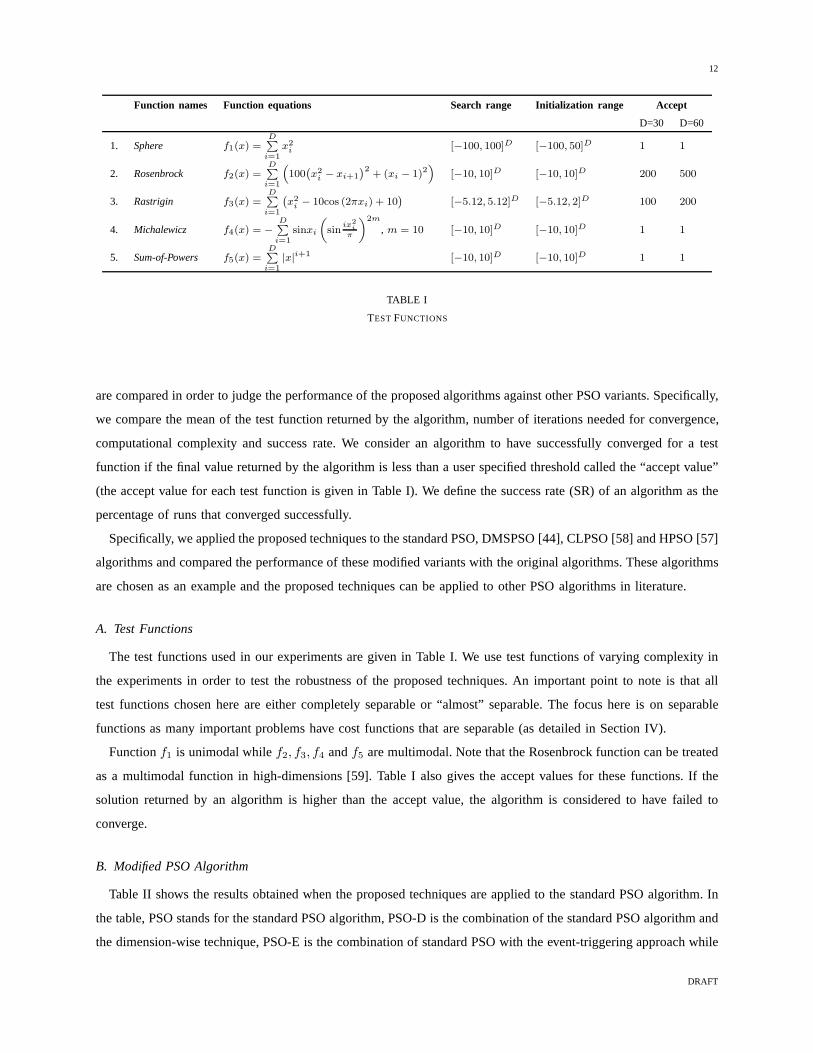
Function names Function equations Search range Initialization range Accept

D=30 D=60

1. Sphere f1(x) =D∑

i=1

x2i

[−100, 100]D [−100, 50]D 1 1

2. Rosenbrock f2(x) =D∑

i=1

(

100(

x2i− xi+1

)2+ (xi − 1)2

)

[−10, 10]D [−10, 10]D 200 500

3. Rastrigin f3(x) =D∑

i=1

(

x2i− 10cos (2πxi) + 10

)

[−5.12, 5.12]D [−5.12, 2]D 100 200

4. Michalewicz f4(x) = −D∑

i=1

sinxi

(

sinix

2

i

π

)2m

, m = 10 [−10, 10]D [−10, 10]D 1 1

5. Sum-of-Powers f5(x) =D∑

i=1

|x|i+1 [−10, 10]D [−10, 10]D 1 1

TABLE I

TEST FUNCTIONS

are compared in order to judge the performance of the proposed algorithms against other PSO variants. Specifically,

we compare the mean of the test function returned by the algorithm, number of iterations needed for convergence,

computational complexity and success rate. We consider an algorithm to have successfully converged for a test

function if the final value returned by the algorithm is less than a user specified threshold called the “accept value”

(the accept value for each test function is given in Table I).We define the success rate (SR) of an algorithm as the

percentage of runs that converged successfully.

Specifically, we applied the proposed techniques to the standard PSO, DMSPSO [44], CLPSO [58] and HPSO [57]

algorithms and compared the performance of these modified variants with the original algorithms. These algorithms

are chosen as an example and the proposed techniques can be applied to other PSO algorithms in literature.

A. Test Functions

The test functions used in our experiments are given in TableI. We use test functions of varying complexity in

the experiments in order to test the robustness of the proposed techniques. An important point to note is that all

test functions chosen here are either completely separableor “almost” separable. The focus here is on separable

functions as many important problems have cost functions that are separable (as detailed in Section IV).

Functionf1 is unimodal whilef2, f3, f4 andf5 are multimodal. Note that the Rosenbrock function can be treated

as a multimodal function in high-dimensions [59]. Table I also gives the accept values for these functions. If the

solution returned by an algorithm is higher than the accept value, the algorithm is considered to have failed to

converge.

B. Modified PSO Algorithm

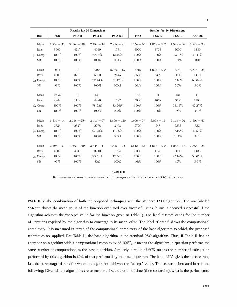
Table II shows the results obtained when the proposed techniques are applied to the standard PSO algorithm. In

the table, PSO stands for the standard PSO algorithm, PSO-D is the combination of the standard PSO algorithm and

the dimension-wise technique, PSO-E is the combination of standard PSO with the event-triggering approach while

DRAFT

13

Results for 30 Dimensions Results for 60 Dimensions

f(x) PSO PSO-D PSO-E PSO-DE PSO PSO-D PSO-E PSO-DE

Mean 1.25e− 32 5.08e− 308 7.18e− 14 7.86e− 21 1.15e− 10 1.07e− 307 1.52e− 08 1.24e− 20

Iters. 5000 4717 4069 1771 5000 4725 5000 1889

f1 Comp. 100% 100% 79.37% 43.46% 100% 100% 96.10% 43.47%

SR 100% 100% 100% 100% 100% 100% 100% 100

Mean 25.2 0 29.3 5.07e− 13 6.06 1.67e− 308 3.57 3.81e− 23

Iters. 5000 3217 5000 2545 3598 3369 5000 1410

f2 Comp. 100% 100% 97.76% 51.47% 100% 100% 97.39% 53.64%

SR 98% 100% 100% 100% 66% 100% 56% 100%

Mean 47.75 0 44.6 0 133 0 131 0

Iters. 4848 1114 4289 1197 5000 1078 5000 1183

f3 Comp. 100% 100% 78.22% 42.26% 100% 100% 93.15% 42.27%

SR 100% 100% 100% 100% 100% 100% 98% 100%

Mean 1.33e− 14 2.65e− 254 2.41e− 07 2.89e− 126 1.06e− 07 3.89e− 45 9.14e− 07 1.30e− 45

Iters. 2335 2337 2268 3198 2720 248 2335 333

f4 Comp. 100% 100% 97.78% 44.89% 100% 100% 97.92% 48.51%

SR 100% 100% 100% 100% 100% 100% 100% 100%

Mean 2.19e− 51 1.36e− 308 3.34e− 17 1.65e− 22 3.51e− 15 1.60e− 308 1.06e− 15 7.85e− 23

Iters. 5000 4541 3910 1194 5000 4175 5000 1438

f5 Comp. 100% 100% 90.51% 42.56% 100% 100% 97.09% 53.63%

SR 90% 100% 82% 100% 46% 100% 42% 100%

TABLE II

PERFORMANCE COMPARISON OF PROPOSED TECHNIQUES APPLIED TO STANDARD PSOALGORITHM .

PSO-DE is the combination of both the proposed techniques with the standard PSO algorithm. The row labeled

“Mean” shows the mean value of the function evaluated over successful runs (a run is deemed successful if the

algorithm achieves the “accept” value for the function given in Table I). The label “Iters.” stands for the number

of iterations required by the algorithm to converge to its mean value. The label “Comp.” shows the computational

complexity. It is measured in terms of the computational complexity of the base algorithm to which the proposed

techniques are applied. For Table II, the base algorithm is the standard PSO algorithm. Thus, if Table II has an

entry for an algorithm with a computational complexity of100%, it means the algorithm in question performs the

same number of computations as the base algorithm. Similarly, a value of60% means the number of calculation

performed by this algorithm is60% of that performed by the base algorithm. The label “SR” givesthe success rate,

i.e., the percentage of runs for which the algorithm achieves the “accept” value. The scenario simulated here is the

following: Given all the algorithms are to run for a fixed duration of time (time constraint), what is the performance

DRAFT

14

Results for 30 Dimensions Results for 60 Dimensions

f(x) DMS DMS-D DMS-E DMS-DE DMS DMS-D DMS-E DMS-DE

Mean 4.73e− 17 5.11e− 308 9.57e− 14 5.26e− 21 6.72e− 05 1.03e− 307 1.46e− 03 1.15e− 20

f1 Iters. 5000 4215 4969 2004 5000 4233 5000 2142%

Comp. 100% 100% 90.80% 43.48% 100% 100% 95.38% 43.45%

SR 100% 100% 100% 100% 100% 100% 100% 100%

Mean 24.2 0 31.9 2.55e− 13 64.6 0 97.6 5.41e− 13

f2 Iters. 5000 4147 5000 3443 5000 4093 5000 3266

Comp. 100% 100% 95.43% 54.58% 100% 100% 95.63% 53.81%

SR 100% 100% 100% 100% 100% 100% 90% 100%

Mean 16.8 0 27.8 0 50.4 0 92 0

f3 Iters. 5000 1172 5000 1172 5000 1139 5000 1185

Comp. 100% 100% 96.67% 42.29% 100% 100% 96.78% 42.28%

SR 100% 100% 100% 100% 100% 100% 100% 100%

Mean 1.61e− 15 4.09e− 309 4.28e− 08 4.72e− 309 6.72e− 15 7.66e− 309 1.23e− 07 6.51e− 156

f4 Iters. 4437 1111 4476 1135 4458 1445 4504 1116

Comp. 100% 100% 97.29% 43.37% 100% 100% 97.19% 44.22%

SR 100% 100% 100% 100% 100% 100% 100% 100%

Mean 7.51e− 28 1.18e− 308 5.99e− 17 1.79e− 22 1.07e− 07 1.61e− 308 1.33e− 01 4.53e− 22

f5 Iters. 5000 4144 4925 1806 5000 5000 5000 1569

Comp. 100% 100% 93.95% 42.54% 100% 100% 95.44% 56.02%

SR 100% 100% 100% 100% 100% 100% 78% 100%

TABLE III

PERFORMANCE COMPARISON OF PROPOSED TECHNIQUES APPLIED TODMSPSOALGORITHM .

of each algorithm with respect to power consumption (measured by computational complexity), accuracy (measured

by mean value) and convergence (measured by success rate)?

Considering the results for the30-D case in Table II, we see that the PSO-D variant significantly enhances

the mean performance of the PSO algorithm. It also speeds up the convergence of the algorithm. The PSO-E

variant has slightly lower computational complexity as compared to the standard PSO at the cost of degraded mean

performance. The results of the PSO-DE variant are of particular interest. The results show that with the exception

of f4, PSO-DE not only converges faster than the PSO algorithm forall test functions but also has a lower mean

value along with a significant reduction in computational cost. For functionf4, PSO-DE has a much lower cost

(2.89e−126 as opposed to1.33e−14) and lower computational complexity (44.89%), although it takes a bit longer

than standard PSO (3198 iterations as opposed to2335) to reach its final value. Nevertheless, it still requires less

computations than the PSO algorithm. The result forf2 and f3 are also significant in that both the PSO-D and

DRAFT

15

PSO-DE variants significantly improve the mean value performance of the original PSO algorithm. Similar trends

are observed for the60-D case. We also note that both the speed of convergence and the reduction in computation

of the PSO-DE algorithm exhibit robustness to increase in the number of dimensions.

C. A Modified DMSPSO Algorithm

Table III shows the30-D and60-D results when the proposed techniques are applied to the DMSPSO algorithm

[44]. In this table, the computational complexity is calculated with respect to the original DMSPSO algorithm.

We observe similar trends as in the case of the standard PSO algorithm. The DMS-D algorithm has a much

improved mean performance as compared to the DMSPSO algorithm as well as much faster convergence. The

DMS-E algorithm offers some reduction in the computationalcomplexity (approximately3% to 9%) at the cost of

degraded performance. The DMS-DE algorithm, however, offer much faster convergence (2 to 4 times faster) and

much lower mean performance (except forf5) at only about half the computational cost. The mean performance

of the PSO-DE algorithm is particularly significant forf2 andf3 as these two functions are considered very hard

to optimize. For the DE variant, the mean performance of the DMS algorithm is improved from24.2 and16.8 to

2.55e− 13 and0 for these two functions, respectively.

In the60-D case, the DMS-E algorithm has a SR of90% and78% for Rosenbrock (f2) and Sum of Powers (f5)

functions respectively. The reason behind this is that the event-triggering approach, in order to save computations,

skips calculating the cognitive and social terms if the particle’s current position is close to its local or global best

respectively. As a result, its mean performance will be lessaccurate than the base algorithm. The DMS algorithm

itself has a mean error performance of64.4 for the Rosenbrock function so it is expected that the DMS-E will

have lower mean performance than the DMSPSO algorithm. Similarly, the Sum of Powers function is known to be

difficult to optimize. High dimensionality coupled with thehighly complex nature of these functions are the cause

of less than100% SR of the DMS-E algorithm.

The DMS-DE variant, however, performs very well for all functions including the Rosenbrock and Sum of

Powers. It gives a much better mean performance than the DMS algorithm for almost all test cases; with less than

half the computations and significant reduction (2− 4 times) in convergence time.

D. A Modified CLPSO Algorithm

Table IV shows the results obtained by applying the two techniques to the CLPSO algorithm [58]. We note that

the CLPSO has been shown to have remarkable performance. TheCLPSO-E variant offers saving in computational

complexity (the computational complexity is measured relative to the original CLPSO algorithm) at the cost of

lower mean performance. The performance of the CLPSO-DE algorithm is similar with its key features being faster

convergence and lower computational cost at the sacrifice ofsuperior mean performance. The mean performance

of the CLPSO-D variant is comparable to the CLPSO algorithm.This is in contrast to the other algorithms tested

(standard PSO, DMSPSO, and HPSO) where the D variant of thosealgorithms considerably improved their mean

performance. The reason behind this is the highly randomized search behavior of the CLPSO where each particle

DRAFT

16

Results for 30 Dimensions Results for 60 Dimensions

f(x) CLPSO CLPSO-D CLPSO-E CLPSO-DE CLPSO CLPSO-D CLPSO-E CLPSO-DE

Mean 1.67e− 309 5.52e− 308 6.03e− 14 6.48e− 20 2.32e− 309 1.07e− 307 1.39e− 13 1.24e− 19

f1 Iters. 4047 4012 1210 1073 4088 3964 1150 1011

Comp. 100% 100% 42.48% 42.40% 100% 100% 42.45% 42.37%

SR 100% 100% 100% 100% 100% 100% 100% 100%

Mean 28.4 163 28.5 162 58.1 372 58.1 397

f2 Iters. 653 407 634 418 4569 4744 1615 4520

Comp. 100% 100% 43.59% 43.58% 100% 100% 43.11% 43.10%

SR 100% 68% 100% 56% 100% 84% 100% 88%

Mean 0 0 1.16e− 11 0 5.78e− 14 0 1.16e− 11 0

f3 Iters. 935 840 1048 747 1014 858 1105 756

Comp. 100% 100% 41.63% 41.53% 100% 100% 41.58% 41.50%

SR 100% 100% 100% 100% 100% 100% 100% 100%

Mean 4.27e− 295 4.57e− 309 2.07e− 205 4.12e− 309 2.41e− 11 7.46e− 309 1.11e− 12 2.26e− 204

f4 Iters. 2275 985 2128 999 630 1017 480 1010

Comp. 100% 100% 43.17% 41.77% 100% 100% 42.61% 41.73%

SR 100% 100% 100% 100% 100% 100% 100% 100%

Mean 1.71e− 309 1.50e− 308 2.23e− 21 2.05e− 21 1.66e− 309 1.77e− 308 4.85e− 21 1.26e− 21

f5 Iters. 4017 3991 1119 998 3965 3956 1231 1119

Comp. 100% 100% 41.77% 41.74% 100% 100% 41.72% 41.71%

SR 100% 100% 100% 100% 94% 100% 88% 100%

TABLE IV

PERFORMANCE COMPARISON OF PROPOSED TECHNIQUES APPLIED TOCLPSOALGORITHM .

learns from different particles for its different dimensions resulting in superior performance and compared to other

PSO algorithms.

E. A Modified HPSO Algorithm

Next we take a look at the effect of the techniques on the HPSO algorithm [57]. The results are tabulated in

Table V. We note that the proposed techniques result in improved performance for all test cases. Specifically for the

Rosenbrock function, we note that all the proposed variantsgreatly improve the mean performance of the HPSO

algorithm.

Although the results of the proposed D and DE variants are very promising, there is one important aspect in which

the proposed DE scheme does not seem to be effective. While the combined effect of the proposed DE scheme

has significantly reduced the number of computations for other PSO variants compared with the event-triggering

DRAFT

17

Results for 30 Dimensions Results for 60 Dimensions

f(x) HP HP-D HP-E HP-DE HP-DE2 HP HP-D HP-E HP-DE HP-DE2

Mean 1.44e−36 6.04e−308 7.69e−11 8.71e−21 1.33e−14 3.99e−22 1.17e−307 8.48e−09 1.59e−20 2.64e−14

f1 Iters. 5000 3425 4987 4997 85 5000 3594 5000 4999 86

Comp. 100% 100% 85.16% 95.36% 0.62% 100% 100% 86% 95.36% 0.62%

SR 100% 100% 100% 100% 100% 100% 100% 100% 100% 100%

Mean 25.5 6.93e−11 23.8 1.12e−12 9.62e−06 73.8 3.24e−10 81.5 2.54e−12 3.65e−2

f2 Iters. 5000 4244 5000 4995 587 5000 3791 5000 5000 1956

Comp. 100% 100% 78.32% 93.94% 14.35% 100% 100% 80.94% 94% 14.35%

SR 100% 100% 100% 100% 100% 100% 100% 100% 100% 100%

Mean 15.3 0 5.06 0 2.06e−12 42.3 0 22.3 0 4.05e−12

f3 Iters. 5000 151 5000 230 1002 5000 153 5000 206 898

Comp. 100% 100% 92.84% 94.93% 3.12% 100% 100% 92.17% 94.93% 3.11%

SR 100% 100% 100% 100% 100% 100% 100% 100% 100% 100%

Mean 3.20e−06 3.49e−264 1.81e−05 4.14e−153 4.99e−87 1.59e−05 6.45e−251 2.12e−05 2.60e−139 1.06e−88

f4 Iters. 4996 1194 4964 4571 3276 4965 1447 4918 4562 2709

Comp. 100% 100% 99.72% 95.73% 19.01% 100% 100% 99% 96.07% 22.74%

SR 100% 100% 100% 100% 100% 100% 100% 100% 100% 100%

Mean 1.61e−29 5.46e−308 8.08e−16 1.72e−22 4.31e−16 4.34e−25 7.86e−308 1.33e−15 3.83e−22 4.48e−16

f5 Iters. 5000 3493 5000 4991 66 5000 3182 4998 4886 65

Comp. 100% 100% 91.20% 94.89% 0.55% 100% 100% 87.49% 93.04% 17.89%

SR 100% 100% 100% 100% 100% 100% 100% 100% 100% 100%

TABLE V

PERFORMANCE COMPARISON OF PROPOSED TECHNIQUES APPLIED TOHPSOALGORITHM .

cases, the result is the opposite in case of HPSO. As shown in Table V, the computational cost of the HPSO-DE

algorithm is about90% of the HPSO algorithm for all functions. The reason behind this is the behavior of the

HPSO algorithm. If the velocity of any of the particles goes to zero, the algorithm re-initializes the particle so that

it keeps moving until the experiment ends. Therefore, we go one step further in the case of HPSO and propose

that the random re-initialization step be performed only ifthe particle has stopped of its own accord rather than

being forced to stop by our techniques. We call this as the HPSO-DE2 variant. As a result of this extra step, we

achieve remarkable results for HPSO. The results show that for the HPSO-DE2 algorithm, the computations reduce

to between1%−20% of the HPSO algorithm whereas for the HPSO-DE the computations are in the range of90%.

These results showcase the remarkable potential of the proposed techniques.

F. Comparison of Convergence Times

The time required by an algorithm to reach a specified error threshold is of particular interest for time-critical

and power-limited applications. Here we present a comparative analysis of the speed of convergence of the various

algorithms to a specified error threshold. We compare the standard PSO, DMSPSO, CLPSO and HPSO along with

their respective DE variants. Note that we use the HPOS-DE2 variant as it is more computationally efficient. We

present results for two error thresholds,1e− 10 and1e− 15. Table VI shows the number of iterations needed by

DRAFT

18

f(x) Threshold PSO DMS CLPSO HPSO PSO-DE DMS-DE CLPSO-DE HPSO-DE2

f11e− 10 3685 4633 762 2025 483 424 389 44

1e− 15 4044 4884 913 2600 768 675 665 ×

f21e− 10 × × × × 1806 2115 × ×

1e− 15 × × × × × × × ×

f31e− 10 × × 763 × 463 663 385 83

1e− 15 × × 870 × 822 1055 590 ×Results

for

30-Df4

1e− 10 1923 1906 224 × 2 2 2 2

1e− 15 2072(40%) 2432(74%) 260 × 3 2 3 3

f51e− 10 2887(90%) 3777 514 1086 20 31 245 32

1e− 15 3278(90%) 4400 720 2223 65 83 559 50

f11e− 10 4931(68%) × 805 3037 582 550 384 45

1e− 15 × × 953 3818 910 871 659 ×

f21e− 10 4277(62%) × × × 16 2095 × ×

1e− 15 4756(42%) × × × 50 × × ×

f31e− 10 × × 810(98%) × 534 709 385 94

1e− 15 × × 913(98%) × 913 1111 554 ×Results

for

60-Df4

1e− 10 1988(92%) 2044 318(94%) × 2 2 2 2

1e− 15 2098(28%) 2459(56%) 356(94%) × 3 3 3 3

f51e− 10 4239(46%) 4970(10%) 571(94%) 1815 25 34 254 33

1e− 15 4814(44%) × 767(94%) 2912 72 91 562 51

TABLE VI

COMPARISON OF CONVERGENCE SPEED OFPSO, DMS, CLPSO, HPSOAND THEIR VARIANTS .

these algorithms to reach the specified error thresholds. These results are averaged over50 runs. For algorithms

that do not reach the specified error threshold for all50 runs, the unsuccessful runs are excluded when calculating

the convergence speed. For such cases, the value in bracket indicates the percentage of successful runs. An ’×’

indicates that the algorithm failed to meet the error threshold for all 50 runs.

The results show that not only do the DE variants converge much faster than the original algorithms, they

also improve the success rate (PSO and PSO-DE for30 and 60 dimensions cases, CLPSO and CLPSO-DE for

60 dimensions case). Moreover, in some instances the originalalgorithm fails while its DE variant successfully

converges to a solution, e.g., PSO-DE and DMS-DE forf2. For f4, the DE variants are able to converge in a

DRAFT

19

f(x) f1 f3 f5

Values Mean Iters. Comp. Mean Iters. Comp. Mean Iters. Comp.

PSO 7.1e−2 500 100% 55.44 500 100% 5.62e−8(88%) 500 100%

PSO-D 5.70e−53 500 100% 0 264 100% 7.18e−86 500 100%

PSO-DE 6.35e−20 412 70.33% 0 293 66.90% 4.32e−21 380 67.76%

DMS 0.71(2%) 500 100% 37.97 500 100% 2.28e−4 500 100%

DMS-D 3.64e−54 500 100% 0 273 100% 3.07e−61 490 100%

DMS-DE 3.85e−20 392 69.88% 0 320 66.48% 1.81e−21 274 67.40%

CL 1.05e−47 500 60% 0 312 60% 1.90 e−51 500 60%

CL-D 3.48e−51 500 60% 0 279 60% 1.25e−53 500 60%

CL-DE 7.19e−19 319 39.24% 0 258 37.63% 2.09e−20 299 37.99%

HP 1.048e−5 500 80% 29.56 500 80% 5.78e−12 500 80%

HP-D 4.90e−111 500 80% 0 87 80% 1.63e−122 500 80%

HP-DE2 5.21e−15 55 3.99% 1.18e−13 227 12.80% 1.85e−16 53 3.62%

TABLE VII

COMPARISON FOR500 ITERATIONS (30-D CASE)

remarkably fast time, i.e.,2− 3 iterations.

CLPSO is faster as compared to the standard PSO algorithm andgenerally has better performance. The modified

PSO-DE not only outperforms the standard PSO but even the CLPSO algorithm in terms of convergence time

to reach the set thresholds as shown in Table VI. The results show that the proposed techniques improved the

convergence times of all the PSO algorithms tested in this study, thereby increasing their scope for time critical

applications.

G. Robustness to Dimensionality

Figure 1 shows the mean performance of various algorithms compared with their DE versions against the number

of dimensions of the optimization problem. The figure shows that the mean performance of the DE technique is

very robust to the increase in the number of dimensions of theproblem. This is a very unique feature specific to

the proposed D and DE techniques as nearly all PSO variants inliterature suffer from the curse of dimensionality.

Intuitively, this result makes sense as the dimension-wiseapproach takes care of the “two step forward, one step

backward” problem and allows the particles to retain the best dimensions of a particular solution.

DRAFT

20

f(x) f1 f3 f5

Values Mean Iters. Comp. Mean Iters. Comp. Mean Iters. Comp.

PSO × × × 150.12(98%) 500 100% × × ×

PSO-D 1.26e−53 500 100% 0 273 100% 1e−57 500 100%

PSO-DE 1.46e−19 446 70.29% 0 291 66.94% 1e−21 332 73.67%

DMS × × × 164.86(62%) 500 100% × × ×

DMS-D 1.61e−54 500 100% 0 269 100% 2.09e−59 492 100%

DMS-DE 9.58e−20 420 69.90% 0 304 66.49% 2.16e−21 344 74.21%

CL 6.54e−44 500 60% 1.15 500 60% 5.63e−51(92%) 500 60%

CL-D 2.57e−52 500 60% 0 275 60% 5.63e−52 500 60%

CL-DE 1.42e−18 310 39.19% 0 259 37.59% 1.68e−20 300 37.30%

HP 0.16 500 80% 69.05 500 80% 0.04(98%) 500 80%

HP-D 6.56e−106 500 80% 0 92 80% 6.52e−115 500 80%

HP-DE2 9.94e−15 70 3.98% 1.52e−13 228 12.78% 1.65e−16 53 16.40%

TABLE VIII

COMPARISON FOR500 ITERATIONS (60-D CASE)

Fig. 1. Effect of increasing dimensions on the mean performance of a few exemplary DE variants.

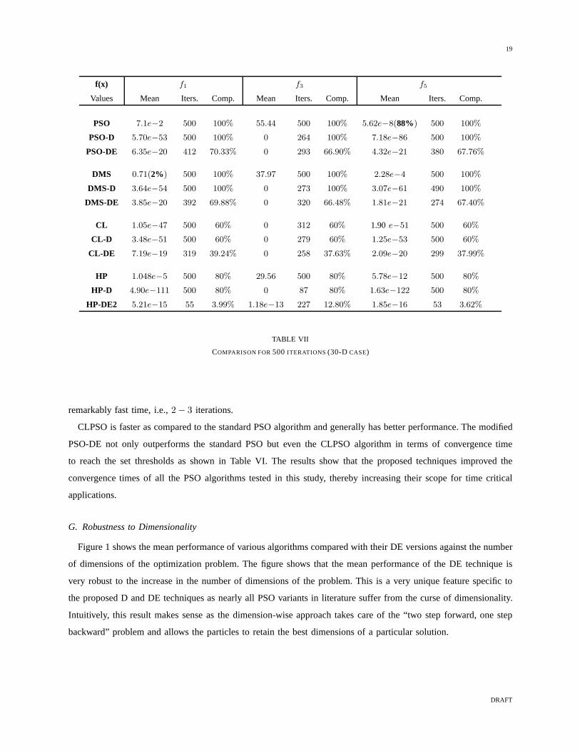
H. A Comparative Study

A slightly different experiment is performed with the aim totest the performance of different PSO algorithms

against their proposed D and DE variants in a scenario where only limited time is available. Instead of running

the simulation for5000 iterations, the number is reduced to only500. The results for3 functions (f1, f3, f5) are

DRAFT

21

tabulated in Tables VII and VIII. The Rosenbrock function has been omitted from this study because the original

versions of all tested algorithms had a considerable highermean performance as compared to their D and DE

variants (except for CLPSO where even the D and DE variants performed poorly). All algorithms performs almost

equally well for the Michalewicz function so the results forthis function have also been omitted. As can be seen

from Tables VII and VIII, almost all algorithms perform poorly for the 3 functions when in their original form.

For the30-dimension case, the D and DE variants of all algorithms outperform their original counterparts in terms

of convergence speed, computational complexity and mean error performance. Only the CLPSO algorithm has a

better mean error performance than its D and DE variants but it still takes longer to converge and has a higher

computational cost. For the60-dimension case, PSO, DMS and HPSO fail to converge for all three test functions

while CLPSO fails forf3. In contrast, their D and DE variants are able to converge in all cases. Application of the

proposed techniques results in significant performance improvement with considerable reduction in computations.

This experiment shows the prowess of the proposed techniques, particularly in time-critical situations.

VII. C ONCLUSION

The paper proposes two techniques for the PSO family of algorithms. The first technique reduces computations

while the second technique increases speed of convergence.The event-triggering approach sacrifices performance

for reduction in computational complexity. The strategy isto calculate the cognitive term of the update equation for

thed-th dimension of a particle only if the distance between thisdimension of the particle’s current position and its

local best is larger than a predefined threshold. Similarly,the social term is calculated only if the distance between

the particle’s current position in thed-th dimension and thed-th dimension of its global best exceeds a threshold.

The dimension-wise technique allows the PSO algorithm to learn from the rich information contained in the various

dimensions of the current positions, and local best positions of its particles. The technique works for separable

functions and minimizes each term of the cost function independently resulting in a much faster convergence. This

does not incur any extra computations as compared to the standard function evaluation procedure. The proposed

techniques can be applied separately or in conjunction to other PSO algorithms presented in literature. Simulation

results show that the application of the proposed techniques to PSO variants improve their convergence speeds and

reduce their computational complexities while still maintaining an acceptable error performance; features that are

desirable for time-critical applications as well as those with power constraints.

REFERENCES

[1] R.C. Eberhart and J. Kennedy, “A new optimizer using particle swarm theory,” inProc. 6th Int. Symp. Micromachine Human Sci., Nagoya,

Japan, pp. 39-43, 1995.

[2] J. Kennedy and R.C. Eberhart, “Particle swarm optimization,” in Proc. IEEE Int. Conf. Neural Networks, Perth, WA, pp. 1942-1948,

1995.

[3] G. Di Carro, F. Ducatelle and L.M. Gambardella, “Swarm intelligence for routing in mobile ad hoc networks,” inProc. IEEE SIS 2005,

pp. 76-83, 2005.

[4] Y. Yuan, Z. He and M. Chen, “Virtual MIMO-based design forwireless sensor networks,”IEEE Trans. Veh. Technol., vol. 55, no. 3, pp.

856-864, 2006.

DRAFT

22

[5] A.T. Al-Awami, W. Saif, A. Zerguine, A. Zidouri and L. Cheded, “An adaptive equalizer based on particle swarm optimization techniques,”

in Proc. ISSPA 2007, Sharjah, UAE, pp. 1-4, 2007.

[6] S. Yogi, K.R. Subhashini, J.K. Sathapathy and S. Kumar, “A novel PSO based adaptive channel equalizer using a modifiedANN structure,”

in Proc. IEEE ICCCCT 2010, Ramanathapuram, India, pp. 442-446, 2010.

[7] S. Yogi, K.R. Subhashini and J.K. Sathapathy, “Equalization of digital communication channels based on PSO algorithm,” in Proc. IEEE

ICCCCT 2010, Ramanathapuram, India, pp. 725-730, 2010.

[8] K.K. Soo, Y.M. Siu, W.S. Chan, L. Yang and R.S. Chen, “Particle-Swarm-Optimization-Based Multiuser Detector for CDMA

Communications,”IEEE Trans. Veh. Technol., vol. 56, no. 5, pp. 3006-3013, 2007.

[9] M.A.S. Choudhry, M. Zubair and I.M. Qureshi, “Particle swarm optimization based MUD for overloaded MC-CDMA system,” in Proc.

IEEE ICWCNIS 2010, Beijing, China, pp. 1-5, 2010.

[10] I. Jouny, “Particle swarm optimization for radar target recognition and modeling,”Proc. SPIE 6967, Automatic Target Recognition XVIII,

69670K (April, 2008); doi:10.1117/12.779092

[11] X. Zeng, Y. Zhang and Y. Guo, “Polyphase coded signal design for MIMO radar using MO-MicPSO,”Jour. Systems Engg. and Electronics,

vol. 22, no. 3, pp. 381-386, 2011.

[12] Y. Xiao, N. Zhang, Z.-W. Wang and K. Kim, “Particle swarmoptimization for MIMO receivers,” inProc. IET ICWMMN 2008, Beijing,

China, pp. 255-259, 2008.

[13] Z.D. Zaharis and T.V. Yioultsis, “A novel adaptive beamforming technique applied on linear antenna arrays using adaptive mutated

boolean PSO,”Progress In Electromagnetics Research, Vol. 117, 165-179, 2011.

[14] Z.-L. Gaing, “Particle swarm optimization to solving the economic dispatch considering the generator constraints,” IEEE Trans. Power

Syst., vol. 18, no. 3, pp. 1187-1195, 2003.

[15] J.-B. Park, K.-S. Lee, J.-R. Shin and K. Lee, “A particleswarm optimization for economic dispatch with nonsmooth cost functions,”

IEEE Trans. Power Sys., vol. 20, no. 1, pp. 34-42, 2005.

[16] B. Zhao, C. Gua and Y. Cao, “A multiagent-based particleswarm optimization approach for optimal reactive power dispatch,” IEEE

Trans. Power Sys., vol. 20, no. 2, pp. 1070-1078, 2005.

[17] T. Victorie and A. Jeyakumar, “Reserve constrained dynamic dispatch of units with valve-point effects,”IEEE Trans. Power Sys., vol.

20, no. 3, pp. 1273-1282, 2005.

[18] A.I. Selvakumar and K. Thanushkodi, “A new particle swarm optimization solution to nonconvex economic dispatch problems,” IEEE

Trans. Power Sys., vol. 22, no. 1, pp. 42-51, 2007.

[19] K.T. Chaturverdi, M. Pandit and L. Srivastava, “Self-organizing hierarchichal particle swamr optimization for nonconvex economic

dispatch,”IEEE Trans. Power Sys., vol. 23, no. 3, pp. 1079-1087, 2008.

[20] N. Jin and Y. Rahmat-Samii, “Advances in particle swarmoptimization for antenna designs: real number, binary, single-objective and

multiobjective implementations,”IEEE Trans. Antennas and Propag., vol. 55, no. 3 I, pp. 556-567, 2007.

[21] D. Boeringer and D. Werner, “Particle swarm optimization versus genetic algorithms for phased array synthesis,”IEEE Trans. Antennas

and Propag., vol. 52, no. 3, pp. 771-779, 2004.

[22] M. Khodier and C. Christodoulou, “Linear array geometry synthesis with minimum sidelobe level and null control using particle swarm

optimization,” IEEE Trans. Antennas and Propag., vol. 53, no. 8, pp. 2674-2679, 2005.

[23] N. Jin and Y. Rahmat-Samii, “Parallel particle swarm optimization and finite-difference time-domain (PSO/FDTD) algorithm for multiband

and wide-band patch antenna designs,”IEEE Trans. Antennas and Propag., vol. 53, no. 11, pp. 3459-3468, 2005.

[24] Z.-L. Gaing, “A particle swarm optimization approach for optimum design of PID controller in AVR system,”IEEE Trans. Energy Conv.,

vol. 19, no. 2, pp. 384-391, 2004.

[25] J. Heo, K. Lee amd R. Garduno-Ramirez, “Multiobjectivecontrol of power plants using particle swarm optimization techniques,”IEEE

Trans. Energy Conv., vol. 21, no. 2, pp. 552-561, 2006.

[26] H. Yoshida, K. Kawata, Y. Fukuyama, S. Takayama and Y. Nakanishi, “A particle swarm optimization for reactive powerand voltage

control considering voltage security assessment,”IEEE Trans. Power Sys., vol. 15, no. 4, pp. 1232-1239, 2000.

[27] M. Abido, “Optimal design of power-system stabilizersusing particle swarm optimization,”IEEE Trans. Energy Conv., vol. 17, no. 3,

pp. 406-413, 2002.

DRAFT

23

[28] K. Veeramachaneni, L. Osadciw and P. Varshney, “An adaptive multimodal biometric management algorithm,”IEEE Trans. Sys., Man

and Cyber. Part C: Apps. and Reviews, vol. 35, no. 3, pp. 344-356, 2005.

[29] S. Kannan, S. Slochanal and N. Padhy, “Application and comparison of metaheuristic techniques to generation expansion planning

problem,” IEEE Trans. Power Sys., vol. 20, no. 1, pp. 466-475, 2005.

[30] J. Robinson and Y. Rahmat-Samii, “Particle swarm optimization in electromagnetics,”IEEE Trans. Antennas and Propag., vol. 52, no.

2, pp. 397-407, 2004.

[31] A. Chatterjee, K. Pulasinghe, K. Watanabe and K. Izumi,“A particle-swarm-optimized fuzzy-neaural network for voice-controlled robot

systems,”IEEE Trans. Ind. Elect., vol. 52, no. 6, pp. 1478-1489, 2005.

[32] L. Messerschmidt and A. Engelbrecht, “Learning to playgames using a PSO-based competitive learning approach,”IEEE Trans. Evol.

Comput., vol. 8, no. 3, pp. 280-288, 2004.

[33] C.-Y. Chen and Y. Fun, “Particle swarm optimization andits application to clustering analysis,” inProc. IEEE Intl. Conf. Networking,

Sensing and Control, 2004, pp. 789-794.

[34] M. Yuwono, S. W. Su, B. Moulton, H. Nguyen, “Fast unsupervised learning method for rapid estimation of cluster centroids,” IEEE

Congress on Evolutionary Computation (CEC), pp.1,8, 10-15 June 2012.

[35] D. W. Van der Merwe, and A. P. Engelbrecht. “Data clustering using particle swarm optimization.”in Proc. of The IEEE Congress on

Evolutionary Computation,, 8-12 Dec., 2003, Canberra, Astralia, pp. 215-220.

[36] R. Poli, “An analysis of publications on particle swarmoptimisation applications,”Tech. Rep. CSM-469, Department of Computing and

Electronic Systems, University of Essex, Colchester, Essex, UK, 2007.

[37] R. Poli, “Analysis of the publications on the applications of particle swarm optimisation,”Jour. Artif. Evo. Appl., vol. 2008, no. 685175,

pp. 1-10, 2008.

[38] Y. Shi and R.C. Eberhart, “Parameter Selection in Particle Swarm Optimization,”Evol. Programming VII, Lec. Notes Comp. Sci., vol.

1447, pp. 591-600, 1998.

[39] M. Clerc and J. Kennedy, “The Particle Swarm - Explosion, Stability, and Convergence in a Multidimensional ComplexSpace,”IEEE

Trans. Evol. Comput., vol. 6, no. 1, pp. 58-73, 2002.

[40] J. Kennedy and R. Mendes, “Population structure and particle swarm performance,” inProc. 2002 CEC, Honolulu, HI, pp. 1671 - 1676,

2002.

[41] T. Peram, K. Veeramachaneni and C. K. Mohan, “Fitness-distance-ratio based particle swarm optimization,” inProc. IEEE Swarm Intell.

Symp., pp. 174-181, 2003.

[42] T.M. Blackwell and J. Branke, “Multi-swarm optimization in dynamic environments,”Apps. Evol. Computing, Lec. Notes Comp. Sci.,

vol. 3005, pp. 489-500, 2004.

[43] M. Lovbjerg, T.K. Rasmussen and T. Krink, “Hybrid particle swarm optimiser with breeding and subpopulations,” inProc. GECCO 2001,

pp. 469-476, 2001.

[44] J.J. Liang and P.N. Suganthan, “Dynamic Multi-Swarm Particle Swarm Optimizer,” inProc. 2005 IEEE Swarm Intell. Symp., pp. 124-129,

2005.

[45] R. Mendes, J. Kennedy and J. Neves, “The Fully Informed Particle Swarm: Simpler, Maybe Better,”IEEE Trans. Evol. Comput., vol. 8,

no. 3, pp. 204-210, 2004.

[46] A. Chatterjee and P. Siarry, “Nonlinear inertia weightvariation for dynamic adaptation in particle swarm optimization,” Computers &

Operations Research, vol. 33, no. 3, pp. 859-871, 2006.

[47] X. Hu and R.C. Eberhart, “Multiobjective optimizationusing dynamic neighborhood particle swarm optimization,”in Proc. 2002 CEC,

Honolulu, HI, pp. 1677-1681, 2002.

[48] K. E. Parsopoulos, M. N. Vrahatis, “UPSO-A unified particle swarm optimization scheme,” inLec. Series Comp. and Comput. Sci., vol.1,

pp. 868-873, 2004.

[49] P. J. Angeline, “Using selection to improve particle swarm optimization,” inProc. IEEE Intl. Conf. Evol. Comput., Anchorage, AK, pp.

84-89, 1998.

[50] V. Miranda and N. Fonseca, “New evolutionary particle swarm algorithm (EPSO) applied to voltage/VAR control,” inProc. 14th Power

Systems Comput. Conf., Seville, Spain, 2002 [online], available at: ¡http://www.pscc02.org/papers/s21pos.pdf¿.

DRAFT

24

[51] M. Lovbjerg and T. Krink, “Extending particle swarm optimizers with self-organized criticality,” inProc. 2002 CEC, Honolulu, HI, 2002,

pp. 1588-1593.

[52] T.M. Blackwell and P.J. Bentley, “Don’t push me! Collision-avoiding swarms,” inProc. 2002 CEC, Honolulu, HI, pp. 1691-1696, 2002.

[53] K.E. Parsopoulos, M.N. Vrahatis, “On the computation of all global minimizers through particle swarm optimization,” IEEE Trans. Evol.

Comput., vol. 8, no. 3, pp. 211-224, 2004.

[54] S.-Y. Ho, H.-S. Lin, W.-H. Liauh, and S.-J. Ho, “OPSO: Orthogonal particle swarm optimization and its application to task assignment

problems,”IEEE Trans. Syst., Man, Cybern. A, vol. 38, no. 2, pp. 288298, 2008.

[55] Z.-H. Zhan, J. Zhang, Y. Li and Y.-H. Shi, “Orthogonal learning particle swarm optimization”,IEEE Trans. Evol. Comput., vol. 15, no.

6, pp. 832-847, 2011.

[56] F. van den Bergh and A. P. Engelbrecht, “A cooperative approach to particle swarm optimization,”IEEE Trans. Evol. Comput., vol. 8,

no. 3, pp. 225-239, 2004.

[57] A. Ratnaweera, S. Halgamuge and H.C. Watson, “Self-organizing hierarchical particle swarm optimizer with time-varying accelerating

coefficients,” IEEE Trans. Evol. Comput., vol. 8, no. 3, pp. 240-255, 2004.

[58] J.J. Liang, A.K. Qin, P.N. Suganthan and S. Baskar, “Comprehensive learning particle swarm optimizer for global optimization of

multimodal functions,”IEEE Trans. Evol. Comput., vol. 10, no. 3, pp. 281-295, 2006.

[59] Y. W. Shang and Y. H. Qiu, “A note on the extended Rosenbrock function,” Evol. Comput., vol. 14, no. 1, pp. 119126, 2006.

DRAFT