1 logistics & supply chain management strategies peerapol sittivijan...
TRANSCRIPT

1
Logistics & Supply Chain Management Strategies
Peerapol Sittivijan
E-mail:[email protected]
August 19, 2009
Guest Lecture at KMUTNB
2
OutlineOutline
• What is supply chain & why it is important?
• The Value of Information: Bullwhip Effect
• Risk Pooling Strategy
• Push, Pull, Push-Pull Strategy
• Distribution Strategy
• Revenue Management

3
Introduction

©Copyright 2003 D. Simchi-Levi
Manufacturing Plants
RegionalWarehouses(DistributionCenters)
Field Wrhs(Dist. Centers)
RetailStores
Customers
A Typical Supply ChainA Typical Supply Chain
Suppliers

©Copyright 2003 D. Simchi-Levi
Example 1: Wal-Mart
Customers Request:Buying detergent,clothes, TV, …...
Wal-Mart Stores
Wal-Mart or third-partydistributioncenters
Procter & Gamble
Plastic ProducerFabric Producer
Da-Fa Clothing, Inc. (China)
SONY Factory (Malaysia)
Electronics Components Producer
Chemical Producer
Zipper Producer
Thread Producer
Plastic Producer
Supply Chain ExamplesSupply Chain Examples

©Copyright 2003 D. Simchi-Levi
Suppliers IC Mfg
PC Board
Subassembly
Suppliers
FAT
US DCs
Europe DCs
Far East DCs
Suppliers
Suppliers
Retailer
Retailer
Retailer
Example 2: Hewlett & Packard (HP)
FAT = Final assembly & testIC Mfg = Integrated circuit manufacturingPC Board = Printed circuit board
Consumers
Consumers
Consumers
Supply Chain Examples (Cont’d)Supply Chain Examples (Cont’d)
©Copyright 2003 D. Simchi-Levi
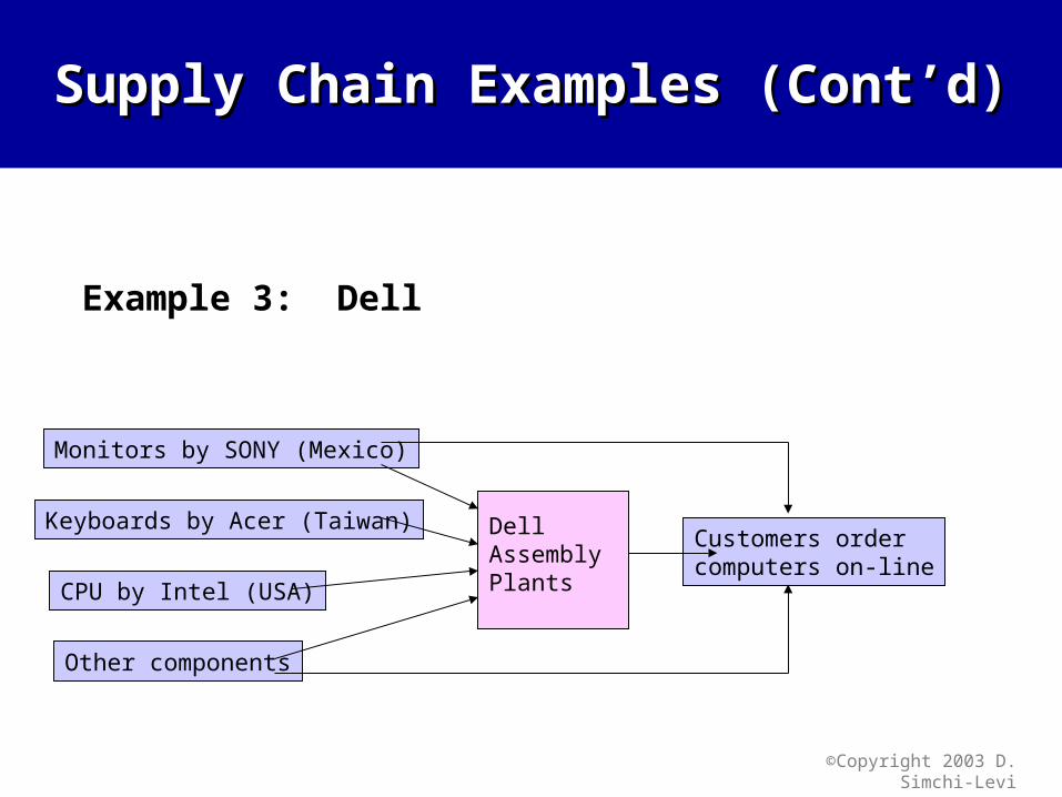
Example 3: Dell
Customers order computers on-line
Dell Assembly Plants
Monitors by SONY (Mexico)
Keyboards by Acer (Taiwan)
CPU by Intel (USA)
Other components
Supply Chain Examples (Cont’d)Supply Chain Examples (Cont’d)

©Copyright 2003 D. Simchi-Levi
• Definition:
Supply Chain Management is primarily concerned with the efficient integration of suppliers, factories, warehouses and stores so that merchandise is produced and distributed in the right quantities, to the right locations and at the right time, and so as to minimize total system cost subject to satisfying service requirements.
• Notice:– Who is involved– Cost and Service Level– It is all about integration
Supply Chain Management

©Copyright 2003 D. Simchi-Levi
Processes Involved in SCMProcesses Involved in SCM
Suppliers Manufacturers Distributors Retailers Consumers
Customer order1. Order arrival (retail stores call/mail order center, website)2. Order entry3. Order fulfillment4. Order receiving
Replenishment1. Retail order trigger (inventory low)2. Retail order entry3. Retail order fulfillment4. Retail order receiving
Manufacturing1. Order arrival from Distr.2. Production scheduling3. Manufacturing & shipping4. Order receiving by Distr.
Procurement1. Order from Mfg2. Supplier production scheduling3. Component manufacturing/shipping4. Order receiving by Mfg

©Copyright 2003 D. Simchi-Levi
TYPICAL DECISIONS
Strategic
Tactical
TYPETIME FRAME
•Supply chain strategies (Sell direct or through retailers? Outsource or in-house? Focus on cost or customer service?)•Supply chain network design (How many plants? Location and capacities of plants and warehouses?)•Product mix at each plant
years
•Workforce & Production planning •Inventory policies (safety stock level)•Which locations supply which markets•Transportation strategies
3 mo.- 1year
Operational•Production scheduling •Distribution scheduling and routing•Place inventory replenishment orders•Lead time quotations
daily
Supply Chain DecisionsSupply Chain Decisions

©Copyright 2003 D. Simchi-Levi
Conflicting local objectives across SC
Manufacturers Distributors Retailers Consumers
Convenience
Short lead time
Large variety of products
Few stores
Low inventory
Little variety
Close to DCs
Low inventory
Few DCs
Large shipments
Large production batches

©Copyright 2003 D. Simchi-Levi
Objective of SCMObjective of SCM
• SCM is concerned with the efficient management of a supply chain so as to maximize supply chain profitability across the entire supply chain
Supply chain profitability = total revenue - total cost
• Manage globally, not locally
• Consider both cost and customer service (Optimal tradeoff between cost and customer service)
(Companies do not compete, their supply chains do)

©Copyright 2003 D. Simchi-Levi
Procurement Planning
ManufacturingPlanning
DistributionPlanning
DemandPlanning
Sequential Optimization
Supply Contracts/Collaboration/Information Systems and DSS
Procurement Planning
ManufacturingPlanning
DistributionPlanning
DemandPlanning
Global Optimization
Sequential Optimization vs. Global Optimization

©Copyright 2003 D. Simchi-Levi
Success for SCM in PracticesSuccess for SCM in Practices
• P&G developed close relationship with their suppliers and jointly created business plans to eliminate wasteful practices across the entire supply chain. As a result, it could save $85 million in 18 months.
• Wal-Mart is the largest and highest-profit retailer in the world by initiating the cross-docking strategy. Goods are continuously delivered to warehouses without ever sitting in inventory.

© Zhi-Long Chen 15
The Value of Information:Bullwhip Effect

©Copyright 2003 D. Simchi-Levi
Information AgeInformation Age
• Internet, Wi-Fi, XML, Web service and Data warehouse
• Provide abundance of available information
• Opportunity to effectively design and manage integrated supply chain
• “In modern supply chain, information replace inventory”

©Copyright 2003 D. Simchi-Levi
The Bullwhip EffectThe Bullwhip Effect
• End-customers’ demand does not vary much, however, inventory and back-order levels considerably fluctuate
• the wholesaler receives orders from the retailer and place orders to the distributor
• Without end-customers’ demand data, the wholesaler use the order from the retailer to perform the forecast and make orders
External Demand
Retailer
Order lead time
Wholesaler
Order lead time
Distributor
Order lead time
Manufacturer
Production lead time
Delivery lead time
Delivery lead time
Delivery lead time
©Copyright 2003 D. Simchi-Levi
The Bullwhip Effect (Cont’d)The Bullwhip Effect (Cont’d)
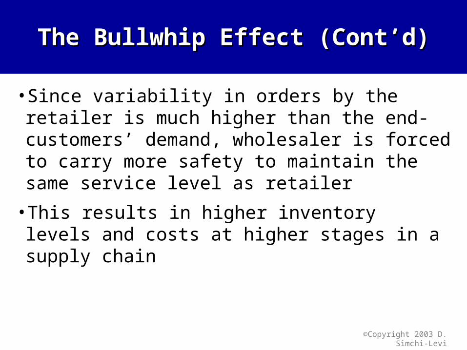
• Since variability in orders by the retailer is much higher than the end-customers’ demand, wholesaler is forced to carry more safety to maintain the same service level as retailer
• This results in higher inventory levels and costs at higher stages in a supply chain

The Bullwhip Effect (Cont’d)The Bullwhip Effect (Cont’d)
©Copyright 2004 D. Simchi-Levi
Ord
er
Siz
e
Time
CustomerDemand
CustomerDemand
Retailer OrdersRetailer OrdersDistributor OrdersDistributor Orders
Production PlanProduction Plan

Example 1: P&G DiapersExample 1: P&G Diapers
©Copyright 2004 D. Simchi-Levi
Lee, H, P. Padmanabhan and S. Wang (1997), Sloan Management Review
©Copyright 2003 D. Simchi-Levi
Factors Affecting VariabilityFactors Affecting Variability
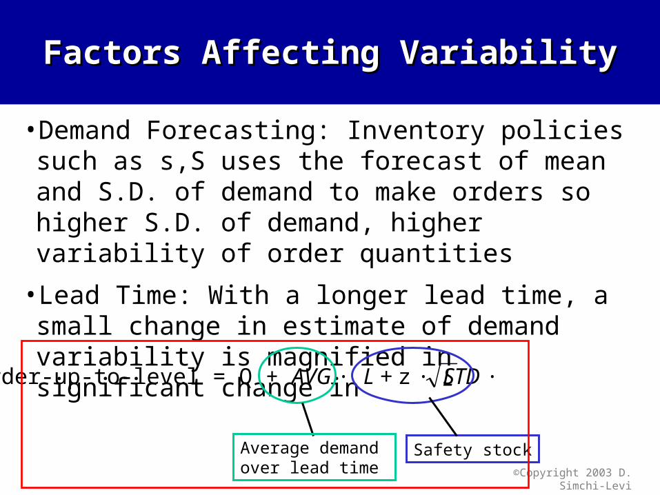
• Demand Forecasting: Inventory policies such as s,S uses the forecast of mean and S.D. of demand to make orders so higher S.D. of demand, higher variability of order quantities
• Lead Time: With a longer lead time, a small change in estimate of demand variability is magnified in significant change in
Order-up-to-level = Q + AVG · L + z · STD · L
Average demand over lead time
Safety stock

©Copyright 2003 D. Simchi-Levi
Factors Affecting Variability (Cont’d)Factors Affecting Variability (Cont’d)
• Batch ordering: A large order followed by several periods of no orders and followed by another period of a large order
• Price fluctuation: Retailers tends to stock up inventories when prices are lower. This can lead to batch ordering
• Inflated orders: Retailers tends to stock up inventories when they suspect that products will be in short supply. This can also lead to distortion of demand estimation
©Copyright 2003 D. Simchi-Levi
Methods to Cope with Bullwhip EffectMethods to Cope with Bullwhip Effect
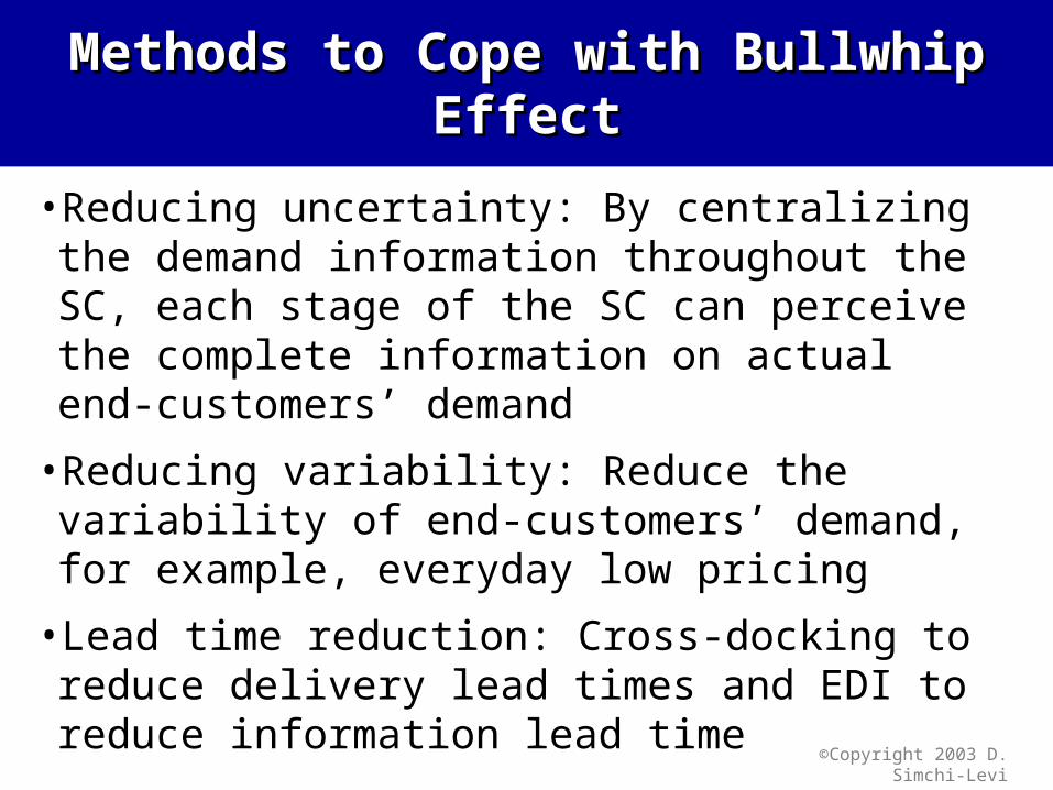
• Reducing uncertainty: By centralizing the demand information throughout the SC, each stage of the SC can perceive the complete information on actual end-customers’ demand
• Reducing variability: Reduce the variability of end-customers’ demand, for example, everyday low pricing
• Lead time reduction: Cross-docking to reduce delivery lead times and EDI to reduce information lead time
©Copyright 2003 D. Simchi-Levi
Centralizing Demand InformationCentralizing Demand Information
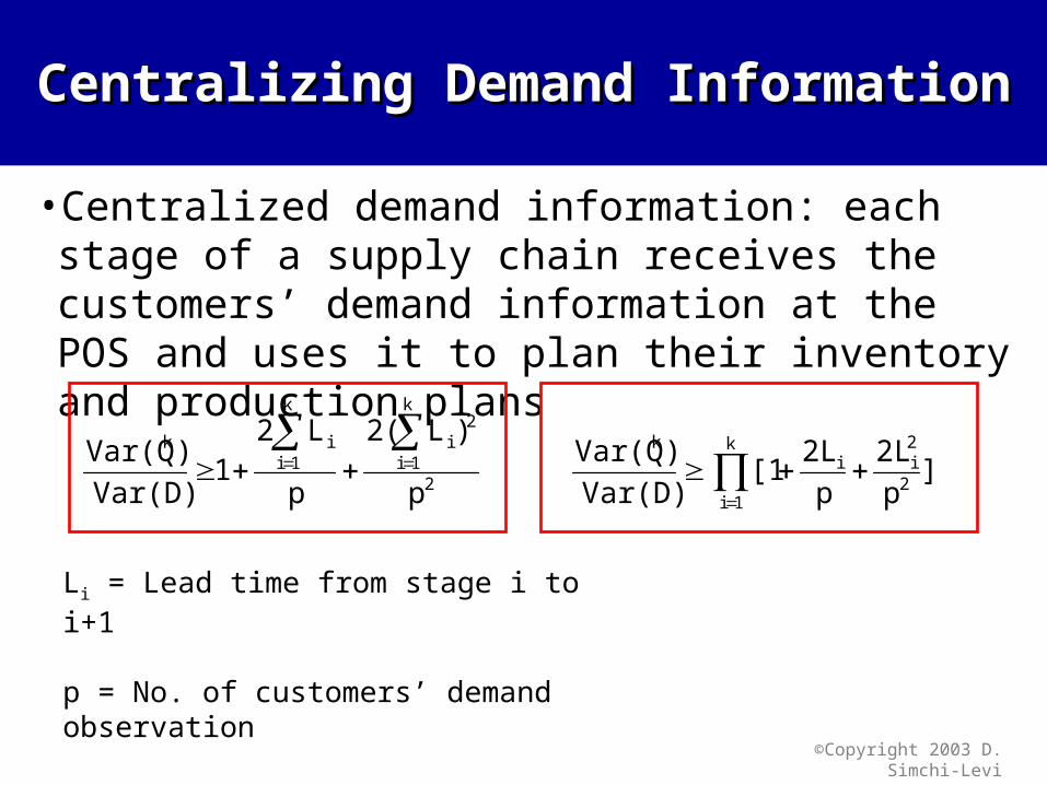
• Centralized demand information: each stage of a supply chain receives the customers’ demand information at the POS and uses it to plan their inventory and production plans
2
k
1i
2i
k
1iik
p
)L2(
p
L2 1
Var(D)
)Var(Q
k
1i2
2ii
k
]p
2L
p
2L [1
Var(D)
)Var(Q
Li = Lead time from stage i to i+1
p = No. of customers’ demand observation

©Copyright 2003 D. Simchi-Levi
Retailer-Supplier PartnershipsRetailer-Supplier Partnerships
• Quick response: suppliers receive POS data from retailers and use it to prepare production and inventory activities, however, the retailers still prepare individual orders
• Continuous replenishment: similar to quick response but suppliers use the data to prepare shipments at predetermined levels of inventory
• Vendor-managed inventory (VMI): the suppliers decide on the appropriate inventory policies
Efficiency Trust

© Zhi-Long Chen 26
Risk Pooling

© Zhi-Long Chen27
Risk PoolingRisk Pooling
• Consider two systems:
Warehouse 1
Warehouse 2
Market 1
Market 2
Supplier
Decentralized System:Two warehouses,each serving one customer
WarehouseMarket 1
Market 2
SupplierCentralized System:One warehouse,serving both customers
Questions: Q1: For the same service level, which system will require more inventory?Q2: For the same total inventory level, which system will have better service?

© Zhi-Long Chen28
• Compare the two systems:– one product– maintain 97% service level– $60 fixed order cost– $0.27 weekly holding cost– 1 week lead time– historical data on demand available (see table on next slide),
assume these data correctly represent demand distributions
Risk PoolingRisk Pooling

© Zhi-Long Chen 29
Risk Pooling ExampleRisk Pooling Example
Week 1 2 3 4 5 6 7 8
Market 1 33 45 37 38 55 30 18 58
Market 2 46 35 41 40 26 48 18 55
Total 79 80 78 78 81 78 36 113
• Historical demand data
© Zhi-Long Chen 30
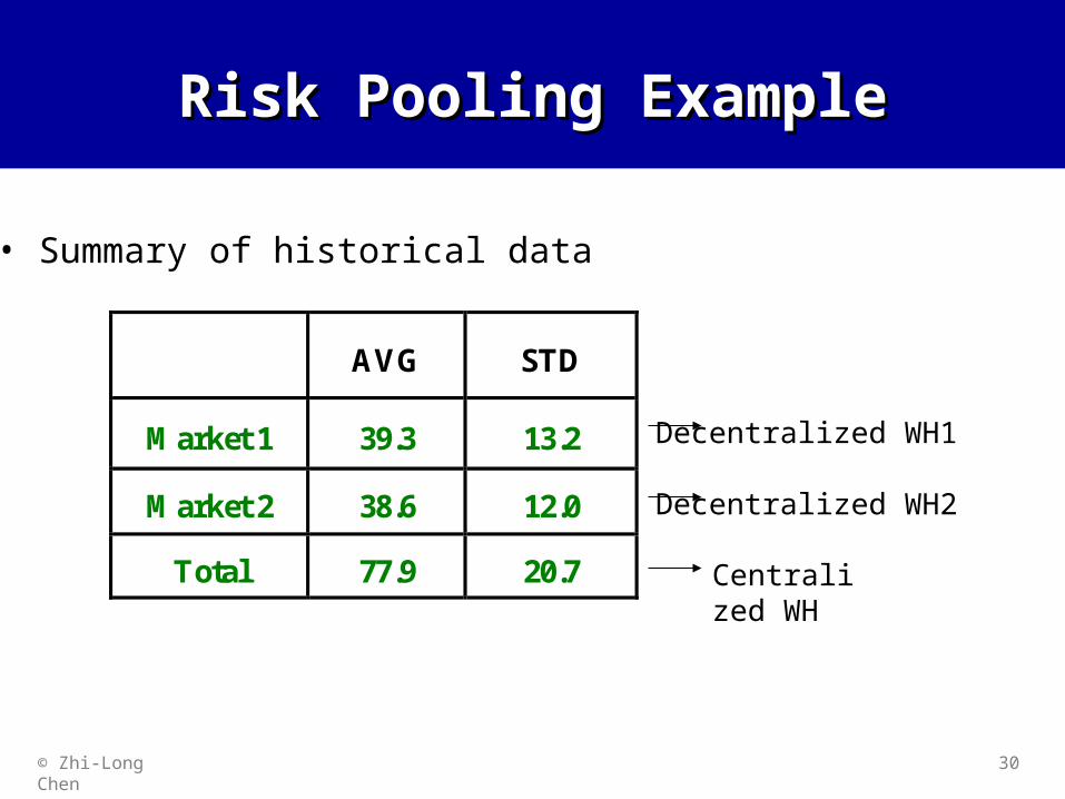
Risk Pooling ExampleRisk Pooling Example
AVG STD
Market 1 39.3 13.2
Market 2 38.6 12.0
Total 77.9 20.7
• Summary of historical data
Decentralized WH1
Decentralized WH2
Centralized WH

© Zhi-Long Chen 31
Given n observations of a random variable, X1, X2, ..., Xn,find mean, variance, and coefficient of variation
M ean n
XX
n
ii
1
V ariance: 1
)(1
2
2
n
XXn
ii
Standard deviat io n: 1
)(1
2
n
XXn
ii
C o effic ient o f var iat io n: X
CV
Excel: Function AVERAGE()
Excel: Function STDEV()
Quick Review of StatisticsQuick Review of Statistics

© Zhi-Long Chen32
(s, S) Policy(s, S) PolicyIn
vent
ory
Lev
el
S
s
0
LeadTimeLeadTime
Inventory Position
Q*
• Use EOQ model to determine optimal order quantity
– Q* =
– Set S = Q* + s
2 K·AVG
hWhereK = setup (ordering) costAVG = mean demand rateh = unit holding cost per unit time
SS

© Zhi-Long Chen 33
More specifically…. More specifically….
• Model with uncertain demand, constant lead timeL = constant lead timeAVG = mean demand rateSTD = stdev of demand rateAssume: Demand rate follows Normal(AVG, STD2)
Reorder point: s = AVG · L + z · STD · L
Average demand over lead time
Safety stock
Answer: Demand over lead time follows Normal(AVG·L, STD2 ·L)
Question: what is the distribution of demand over lead time?

© Zhi-Long Chen 34
Risk Pooling ExampleRisk Pooling Example
AVG STD SS s Q SAverage
Inventory
Warehouse 1 39.3 13.2 25.08 65 132 197 91
Warehouse 2 38.6 12.0 22.8 62 131 193 88
CentralizedWarehouse
77.9 20.7 39.35 118 186 304 132
• Optimal inventory policies
Decentralized system: total SS = 47.88
total avg. invent. = 179
LSS = z ·STD ·s = AVG·L + SSQ = sqrt(2K·AVG/h)
Safety StockReorder PointOrder QuantityOrder-up-to-level S = s + Q
Average Inventory SS + Q/2

© Zhi-Long Chen35
Risk Pooling: Important Risk Pooling: Important ObservationsObservations
• Centralizing inventory control reduces both safety stock and average inventory level for the same service level.
(This phenomenon is called risk pooling)
• Root Cause: Demand Variability (i.e. STD) Variability of aggregated demand is lower than total variability of individual demands
SS = (z)(STD)(sqrt(L))Avg inventory = SS + Q/2
SS = (z)(STD)(sqrt(L))Avg inventory = SS + Q/2
Everything else being equal,a system with a lower demand variability requires a lower SS & lower avg inventory
Everything else being equal,a system with a lower demand variability requires a lower SS & lower avg inventory
Question: Why variability of aggregated demand is lower than total variability of individual demands ?

© Zhi-Long Chen 36
WarehouseMarket 1
Market 2
d1+d2: (, 2)
Calculating demand variability of Calculating demand variability of centralized systemcentralized system
Warehouse 1
Warehouse 2
Market 1
Market 2
d1: (1, 12)
d2: (2, 22)
2 = 1
2 + 22 + 212,
where -1 12
= 12 + 2
2 + 212,
where -1 1
: correlation coefficient of d1, d2
1+ 2 1+ 2
Conclusions: 1. Stdev of aggregated demand is less than the sum of stdev of individual demands2. If demands are independent or negatively correlated, the std of aggregated demand is much less
Conclusions: 1. Stdev of aggregated demand is less than the sum of stdev of individual demands2. If demands are independent or negatively correlated, the std of aggregated demand is much less
1. If d1, d2 positively correlated, > 02. If d1, d2 negatively correlated, < 0
= 1 + 2
= ??
1+2
10-1
22
21
P.C.N.C. Ind.

© Zhi-Long Chen 37
More ObservationsMore Observations
• In general, total safety stock & average inventory both increase with the number of stocking locations
Total SS (Avg. Inv.)
# of stocking locations

© Zhi-Long Chen 38
DecentralizedCentralized
Inbound transportation cost (from factories to warehouses)
Facility/Labor cost
Outbound transportation cost (from warehouses to retailers)
Inventory cost
Responsiveness to customers
Lower
Lower
Higher
Lower
Lower
Centralized vs. DecentralizedCentralized vs. Decentralized

© Zhi-Long Chen39
Critical Points about Risk PoolingCritical Points about Risk Pooling
• Centralizing inventory reduces both safety stock and average inventory in the system.
• The benefits from risk pooling depend on the behavior of demand from one market relative to the demand form another (demand correlations).
• The higher the coefficient of variation, the greater the benefit obtained from centralized system.

© Zhi-Long Chen 40
Push, Pull, Push-Pull Strategy

©Copyright 2003 D. Simchi-Levi
Push StrategyPush Strategy
• Production and distribution decision based on long term forecasts
• Take long time to react to the changing marketplace
• Problems
- Inability to meet changing demand patterns
- Product obsolescence
- Excessive inventories for large safety stock
- Low service levels

©Copyright 2003 D. Simchi-Levi
Pull StrategyPull Strategy
• Production and distribution based on demand driven by fast information flow to transfer demand data
• Coordinate with true customer demand rather than forecast demand
Advantages
- Reduced lead times (better anticipation and coordination)
- Decreased inventory levels at retailers and manufacturers
- Decreased system variability
- Better response to changing markets
disadvantages
- Harder to leverage economies of scale (manufacturing and transportation)
- Doesn’t work in the case that lead times are too long

© David Simchi-Levi
Matching Supply Chain Strategies Matching Supply Chain Strategies with Productswith Products
Pull Push
Pull
Push
I
Computer
II
Furniture, Automobile
IV
Books, CDs
III
Grocery
Demand uncertainty
(C.V.)
Delivery costUnit price
L H
H
L
Economies of Scale

© David Simchi-Levi
Selecting the Best SC StrategySelecting the Best SC Strategy
• Higher demand uncertainty suggests pull• High importance of economies of scale suggests
push• High uncertainty/ EOS not important such as the
computer industry implies pull• Low uncertainty/ EOS important such as groceries
implies push– Demand is stable– Transportation cost reduction is critical– Pull would not be appropriate here.

© David Simchi-Levi
Selecting the Best SC StrategySelecting the Best SC Strategy
• Low uncertainty but low value of economies of scale (high volume books and cd’s)– Either push strategies or push/pull strategies might be most
appropriate
• High uncertainty and high value of economies of scale– For example, the furniture or automobile industry– How can production be pull but delivery push?– Is this a “pull-push” system?
© David Simchi-Levi
Push-Pull StrategyPush-Pull Strategy
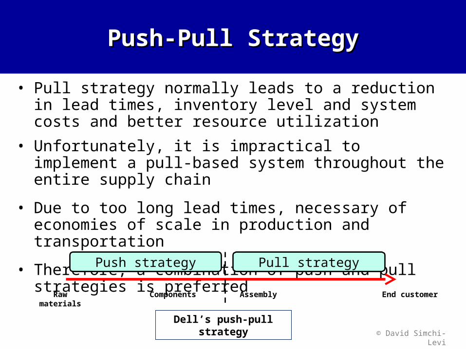
• Pull strategy normally leads to a reduction in lead times, inventory level and system costs and better resource utilization
• Unfortunately, it is impractical to implement a pull-based system throughout the entire supply chain
• Due to too long lead times, necessary of economies of scale in production and transportation
• Therefore, a combination of push and pull strategies is preferred
End customerRaw materials Components Assembly
Push strategy Pull strategy
Dell’s push-pull strategy

© David Simchi-Levi47
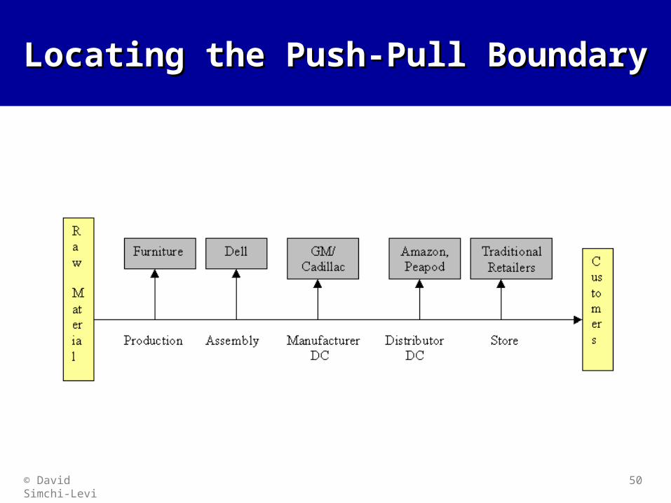
Locating the Push-Pull BoundaryLocating the Push-Pull Boundary
• The push section:– Uncertainty is relatively low– Economies of scale important– Long lead times– Complex supply chain structures
• Thus:– Management based on forecasts is appropriate– Focus is on cost minimization– Achieved by effective resource utilization – supply chain
optimization

© David Simchi-Levi48
•The pull section:–High uncertainty
–Simple supply chain structure
–Short lead times
•Thus–Reacting to realized demand is important
–Focus on service level
–Flexible and responsive approaches
Locating the Push-Pull BoundaryLocating the Push-Pull Boundary
© David Simchi-Levi
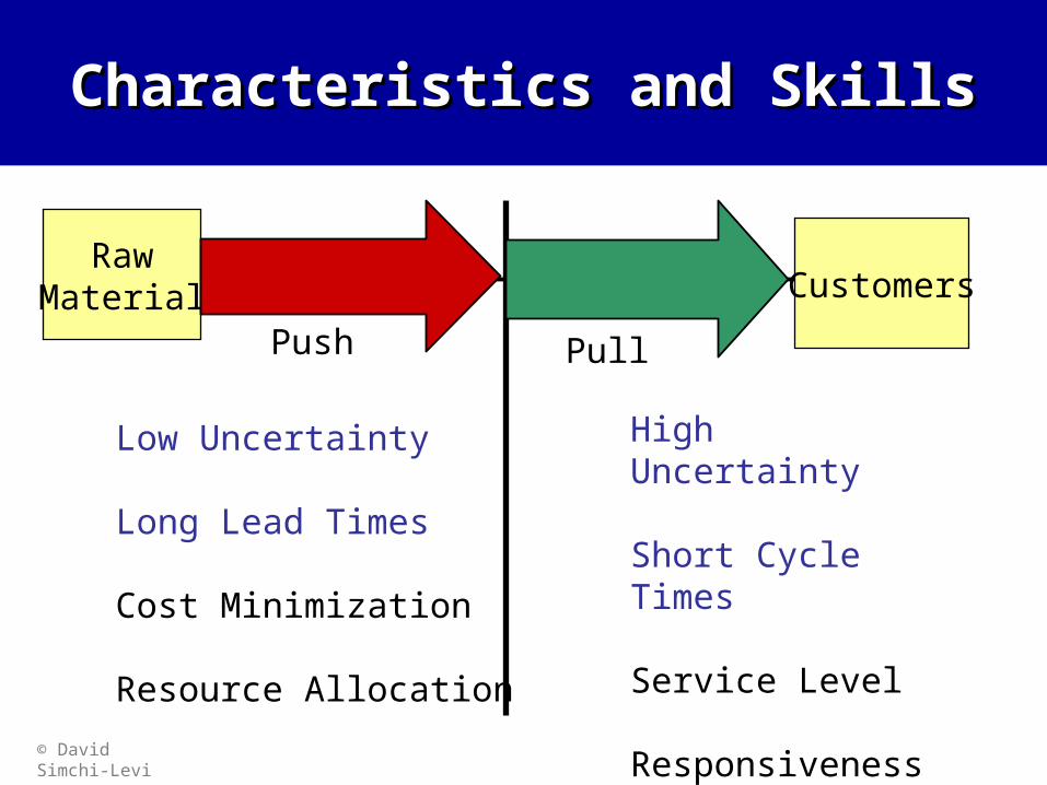
Characteristics and SkillsCharacteristics and Skills
RawMaterial Customers
PullPush
Low Uncertainty
Long Lead Times
Cost Minimization
Resource Allocation
High Uncertainty
Short Cycle Times
Service Level
Responsiveness
© David Simchi-Levi 50
Locating the Push-Pull BoundaryLocating the Push-Pull Boundary

© David Simchi-Levi51
Locating the Push-Pull BoundaryLocating the Push-Pull Boundary
• The push section requires:– Supply chain planning– Long term strategies
• The pull section requires:– Order fulfillment processes– Customer relationship management
• Buffer inventory at the boundaries:– The output of the tactical planning process– The input to the order fulfillment process.

© Zhi-Long Chen 52
Distribution Strategy

© David Simchi-Levi53
Types of Distribution StrategiesTypes of Distribution Strategies
• Direct Shipping
• Shipping via Warehouses
• Shipping via Cross Docks
• Third Party Logistics (3PL)
© David Simchi-Levi54
Direct Shipping (Cont’d)Direct Shipping (Cont’d)
Advantages:
• Avoids the expense of operating a distribution center
• Lead times are reduced
Disadvantages:
• Risk pooling strategy cannot be applied in this case
• Transportation costs of manufacturing and retailer increase because inventory must be sent in smaller volumes (less than truck load)

© David Simchi-Levi55
Shipping Via WarehousesShipping Via Warehouses
Advantages:• Better service from regional locations• Transportation economies• Mixing functions• Risk pooling over the manufacturing or procurement
lead time• Differentiated stocking and service policies
© David Simchi-Levi56
Shipping Via Warehouses (Cont’d)Shipping Via Warehouses (Cont’d)
Design and planning issues:• Number of echelons• Number and location of distribution centers • Stock location: what items to stock at each DC• Replenishment policies – inventory & transportation;
who serves whom• Information systems

© David Simchi-Levi57
Shipping Via Cross docksShipping Via Cross docks
• Warehouses: Receiving, Sorting, Storing, Order Picking, Shipping
• Cross Docks = Warehouses without inventory Receiving, Sorting, Shipping
Sorting
Receiving
Inbound shipments
Shipping
Outbound shipments
Requires coordination & IT supportRequires coordination & IT support

© David Simchi-Levi58
Shipping Via Cross docks (Cont’d)Shipping Via Cross docks (Cont’d)
• Goods spend at most 48 hours in the warehouse
• Cross Docking avoids inventory and handling costs,
• Stores trigger orders for products
• Very difficult to manage
• Requires advanced information technology
• All of Wal-Mart’s distribution centers, suppliers and stores are electronically linked to guarantee that any order is processed and executed in a matter of hours

© David Simchi-Levi59
Shipping Via Cross docks (Cont’d)Shipping Via Cross docks (Cont’d)
• Goods spend at most 48 hours in the warehouse
• Cross Docking avoids inventory and handling costs,
• Stores trigger orders for products
• Very difficult to manage
• Requires advanced information technology
• All of Wal-Mart’s distribution centers, suppliers and stores are electronically linked to guarantee that any order is processed and executed in a matter of hours

© David Simchi-Levi60
Shipping Via Cross docks (Cont’d)Shipping Via Cross docks (Cont’d)
• Wal-Mart operates a private satellite-communications system that sends point-of-sale data to all its vendors allowing them to have a clear vision of sales at the stores
• Needs a fast and responsive transportation system
• Wal-Mart has a dedicated fleet of 2000 truck that serve their 19 warehouses. This allows them to ship goods from warehouses to stores in less than 48 hours replenish stores twice a week on average

© David Simchi-Levi61
Comparing Three StrategiesComparing Three Strategies
W2Factory
W1
W3
Decentralized system: r = 1, L
Safety stock at each warehouse proportional to
Total safety stock
i L 1 3
ii 1
z L 1

© David Simchi-Levi62
Comparing Three Strategies Comparing Three Strategies (Cont’d)(Cont’d)
W2Factory
W1
W3Idealized system: r=1, L
Total safety stock
Safety stock at each warehouse3
2ii3
i 1i
i 1
z L 1
32i
i 1
z L 1

© David Simchi-Levi63
Comparing Three Strategies Comparing Three Strategies (Cont’d)(Cont’d)
W2Factory
W1
W3
Cross-dock system: r = 1, L = L1 + L2
Each period:• System replenishment order = d1 + d2 + d3
• Allocate stock receipts to balance inventories• Transship allocations
L1
L2

© David Simchi-Levi64
Comparing Three StrategiesComparing Three Strategies
Total safety stock
Decentralized
Idealized
Cross-dock
n L 1
n L 1
12
Ln L 1
n
n “identical” warehouses, each with standard deviation of demand =

© Stephen C. Graves 65
L1=0 L1=2 L1=5 L1=8 L1=10 Ideal
n=1 166 166 166 166 166 166
n=2 332 316 292 265 245 235
n=3 497 466 415 357 312 287
n=5 829 766 661 536 433 371
n=10 1658 1517 1275 975 707 524
Safety stock L = 10, = 50, n warehouses with same
Cross-Docking v.s. Idealized SystemCross-Docking v.s. Idealized System

© Stephen C. Graves 66
# of Ws One-echelon Two-echelon
n=1 150 212
n=2 300 342
n=3 450 457
n=4 600 566
n=5 750 671
Decentralized v.s. CDCDecentralized v.s. CDC

© Zhi-Long Chen 67
Revenue Management

©Copyright 2002 D. Simchi-Levi
Revenue ManagementRevenue Management
• Example:– A cruise ship with C=400 identical cabins– The Price-Quantity relationship

©Copyright 2002 D. Simchi-Levi
Revenue ManagementRevenue Management
Price
No. seats
2000
1000
P=2000-2Q

©Copyright 2002 D. Simchi-Levi
RevenueRevenue Management
• Example:– A cruise ship with C=400 identical cabins– The Price-Quantity relationship
• What is the price that the company should charge to maximize revenue?

©Copyright 2002 D. Simchi-Levi
Revenue ManagementRevenue Management
Price
No. seats
P0=1200
C=500
Revenue=480,000

©Copyright 2002 D. Simchi-Levi
Revenue ManagementRevenue Management
Price
No. seats
P0=1200
C=400
Money on the Table=160,000

©Copyright 2002 D. Simchi-Levi
Revenue ManagementRevenue Management
Price
No. seats
P2=1600
Q2=200

©Copyright 2002 D. Simchi-Levi
Revenue ManagementRevenue Management
Price
No. seats
Q1 =400
P1=1200
Q2=200
P2=1600
Revenue=1600(200) + 1200(400-200)=560,000

©Copyright 2002 D. Simchi-Levi
Revenue ManagementRevenue Management
• Can we increase revenue more?

©Copyright 2002 D. Simchi-Levi
Revenue ManagementRevenue Management
Price
No. seats
Q1 =400
P1=1200
Q2=200
P2=1600
P3=1800
Q3=100
Revenue=1800(100) + 1600(200-100) + 1200(400-200)=580,000

©Copyright 2002 D. Simchi-Levi
How can the firm prevent customers How can the firm prevent customers from moving from one class to from moving from one class to
another?another?
Leisure
Travelers
Business
Travelers
No
Offer
No
Demand
Sensitivity to
Price
Sensitivity to Duration
Sensitivity to Flexibility
High Low
Low
High

Mail-in RebateMail-in Rebate
• To differentiate between customers based on their sensitivity to price
• Adding significant hurdle to the buying process; to receive rebate
• Have to complete and mail the coupon to the manufacturer
• Those customers willing to pay the higher price will not necessarily send the coupon

©Copyright 2002 D. Simchi-Levi
• A Retailer and a manufacturer.– Retailer faces customer demand.
– Retailer orders from manufacturer.
Selling Price=?
Wholesale Price=$900
Retailer Manufacturer
Variable Production Cost=$200
ExampleExample

©Copyright 2002 D. Simchi-Levi
Example (Cont’d)Example (Cont’d)
Demand
Price
10000
2000
P=2000-0.2Q
©Copyright 2002 D. Simchi-Levi
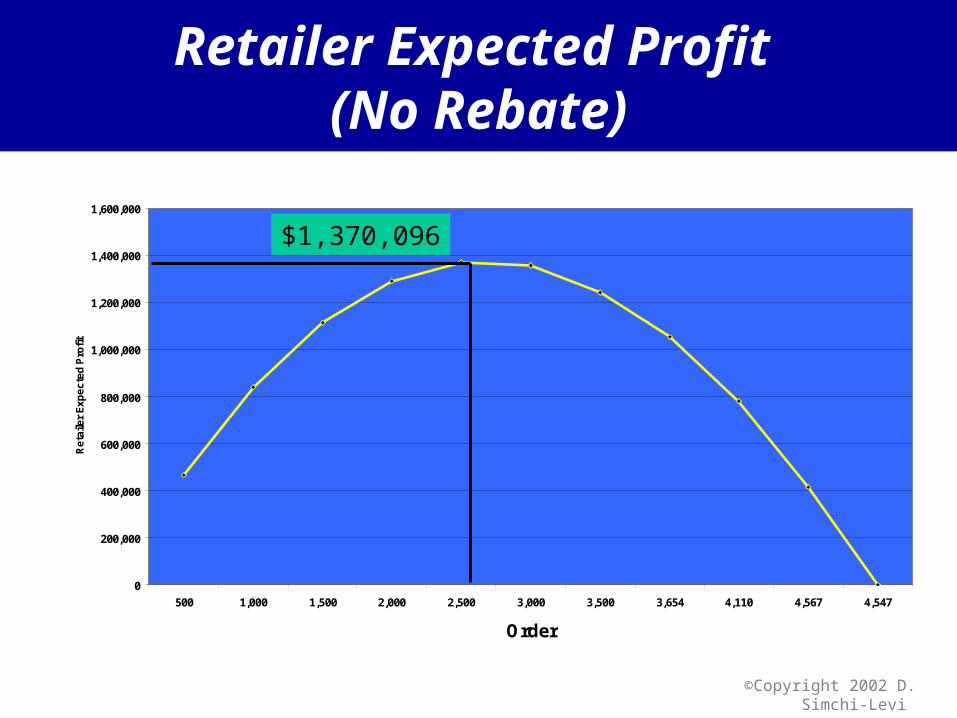
Retailer Expected Profit (No Rebate)
0
200,000
400,000
600,000
800,000
1,000,000
1,200,000
1,400,000
1,600,000
500 1,000 1,500 2,000 2,500 3,000 3,500 3,654 4,110 4,567 4,547
Order
Re
taile
r E
xp
ec
ted
Pro
fit
$1,370,096

©Copyright 2002 D. Simchi-Levi
Manufacturer Profit (No Rebate)
0
1,000,000
2,000,000
3,000,000
4,000,000
5,000,000
6,000,000
500
1,00
01,
500
2,00
02,
500
3,00
03,
500
3,65
44,
110
4,56
74,
547
4,96
15,
374
5,78
86,
201
6,61
47,
028
7,44
17,
855
Order
Man
ufa
ctu
rer
Pro
fit
$1,750,000

©Copyright 2002 D. Simchi-Levi
Example (Cont’d)Example (Cont’d)
Demand
Price
10000
2000
P=2100-0.2Q

©Copyright 2002 D. Simchi-Levi
Retailer Expected Profit ($100 Rebate)
0
200,000
400,000
600,000
800,000
1,000,000
1,200,000
1,400,000
1,600,000
1,800,000
1,000 1,500 2,000 2,500 3,000 3,500 4,000 4,110 4,567 4,547 4,961
Order
Ret
aile
r E
xpec
ted
Pro
fit
$1,644,115

©Copyright 2002 D. Simchi-Levi
Manufacturer Profit ($100 Rebate)
0
1,000,000
2,000,000
3,000,000
4,000,000
5,000,000
6,000,000
1,00
01,
500
2,00
02,
500
3,00
03,
500
4,00
04,
110
4,56
74,
547
4,96
15,
374
5,78
86,
201
6,61
47,
028
7,44
17,
855
8,26
8
Order
Man
ufa
ctu
rer
Pro
fit
$1,810,392

© Zhi-Long Chen86
Main ReferenceMain Reference
• Presentation slides of Prof. Zhi-Long Chen in the course “Supply Chain Strategies”, MIT, Mass, US.
• Simchi-levi, D., Kaminski, P. and Simchi-levi, E. (2004), Chapter 3, “Inventory Management”.
• Simchi-Levi, D., Kaminsky, P. and Simchi-Levi, E. (2003), “Designing and Managing the Supply Chain”, Irwin McGraw Hill, 2nd edition.