1

Liveness analysis andRegister Allocation

Cheng-Chia Chen

The Memory Hierarchy

Registers 1 cycle 256-8000 bytes

Cache 3 cycles 256k-1M

Main memory 20-100 cycles 32M-1G

Disk 0.5-5M cycles 4G-1T

Managing the Memory Hierarchy

• Programs are written as if there are only two kinds of memory: main memory and disk

• Programmer is responsible for moving data from disk to memory (e.g., file I/O)

• Hardware is responsible for moving data between memory and caches

• Compiler is responsible for moving data between memory and registers

Current Trends

• Cache and register sizes are growing slowly• Processor speed improves faster than memory speed

and disk speed– The cost of a cache miss is growing– The widening gap is bridged with more caches

• It is very important to:– Manage registers properly– Manage caches properly

• Compilers are good at managing registers

The Register Allocation Problem

• Recall that intermediate code uses as many temporaries as necessary– This complicates final translation to assembly– But simplifies code generation and optimization– Typical intermediate code uses too many temporaries

• The register allocation problem:– Rewrite the intermediate code to use fewer temporaries than there

are machine registers– Method: assign more temporaries to a register

• But without changing the program behavior

History

• Register allocation is as old as intermediate code• Register allocation was used in the original FORTRAN

compiler in the ‘50s– Very crude algorithms

• A breakthrough was not achieved until 1980 when Chaitin invented a register allocation scheme based on graph coloring– Relatively simple, global and works well in practice

An Example

• Consider the programa := c + de := a + bf := e - 1

– with the assumption that a and e die after use• Temporary a can be “reused” after e := a + b• Same with temporary e• Can allocate a, e, and f all to one register (r1):

r1 := r2 + r3

r1 := r1 + r4

r1 := r1 - 1

Basic Register Allocation Idea

• The value in a dead temporary is not needed for the rest of the computation– A dead temporary can be reused

• Basic rule:

– Temporaries t1 and t2 can share the same register if at any point in the program at most one of t1 or t2 is live !

Algorithm: Part I

• Compute live variables for each point:

a := b + cd := -ae := d + f

f := 2 * eb := d + e

e := e - 1

b := f + c

{b}

{c,e}

{b}

{c,f} {c,f}

{b,c,e,f}

{c,d,e,f}

{b,c,f}

{c,d,f}{a,c,f}

10

Dataflow Equations

• Control-flow graph– Out-edge, in-edge, successor, predicessor

• Use and Def Sets– Use : on the right-hand side of assignment– Def : assignment to a var defines that var.

• Liveness– A variable is “live” on an edge if there is a directed path from that

edge to a use fo the variable that does not go through any def.

11

Control Flow Graph (CFG)

• A control flow graph for a program (or subroutine) is a digraph such that– Each statement (or basic block) in the program is a node in the

CFG.– if statement X can be followed by statement Y, then there is an

edge from X to Y.– e.g., Figure 10.1.

• A variable is live if its current value may be used in the future.– The analysis is backward (from the future to the past).– e.g., b used in S4, => live at edge 3 4, 2 3.– since S2 assign new value to b, content of b from S1 is not used.– the live range of b is { 23, 3 4}.

12

10.1 CFG of a program

a 0L1: b a + 1 c c + b a b * 2 if a < N goto L1 return c.

a := 0

return c

c := c + b

a < N

b := a + 1

a := b * 2

1

2

3

4

5

6

13

Liveness of variable a and b

a := 0

return c

c := c + b

a < N

b := a + 1

a := b * 2

a := 0

return c

c := c + b

a < N

b := a + 1

a := b * 2

var defined

var used

14

Liveness of variable c

a := 0

return c

c := c + b

a < N

b := a + 1

a := b * 2

1

2

3

4

5

6

uninitialized c detected if c is not a formal defined/used

var used

15

predecessor and successor

• If there is an edge E from node X to Node Y, then E is an in-edge of Y and an out-edge of X; Y is said to be a successor of X and X a predecessor of Y.

• For each node n, define– pred[n] = the set of all predecessors of node n and– succ[n] = the set of all successor edges of node n.– e.g., in Figure 10.1, – out-edges of node 5 are: 5 6, 5 2,– in-edges of node 2 are : 5 2, 1 2.– pred[2] = {1,5}; – succ[2] = { 3 }.

16

Uses and defs

• An assignment to a variable or temporary defines the variable.– x y – 2; b a + 3; c f(a,c,b) + 2

• An occurrence of a variable on the right hand side of an assignment (or in other expression) uses the variable.– x y – 2; b a + 3; c f(a,c,b) + 2

• Definition:– def[x] = { n | var x is defined in Node n}– def[n] = { x | var x is defined in node n }.– use[x] = { n | var x is used in Node n}– use[n] = { x | var x is used in node n }.

17

Liveness

• A variable is live on an edge if there is a directed path from that edge to a use of the variable without going through any def.

• A variable is live-in at a node if it is live on any of the in-edges of that node.

• A variable is live-out at a node if it is live on any of the out-edges of that node.

X is live-in atthis node

X is live at this edge X is live-out at this node

X is live at this edge

18

(y1,y2,x3) f(x1,x2,x3).

X is live at all these edge iff

X is used at n (i.e., x1 or x2 or x3).

or X is live at at some out-edge of n and X is not defined at n (i.e., not y1,y2 or x3)

y1,x2z1x3

out[n] = {y1,x2, x3,z1 }

in[n] = use[n] U (out[n]-defs[n]) ={x1,x2,x3} U {x2,z1}

19

Dataflow equations for liveness analysis

• definitions:– in[n] = set of variables that are live-in at node n.– out[n] = set of variables that are live-out at node n.

• Equations for defs, in and out.

1. in[n] = use[n] U (out[n] – def[n] ). – var x is live at an (and all) edge to n iff either– 1. x is used at n or– 2. x is live at an out-edge of n and n does not define x.

2. out[n] = U s succ[n] in[s]– var x live-out at node n iff– var x is live at an edge leaving from n.

20

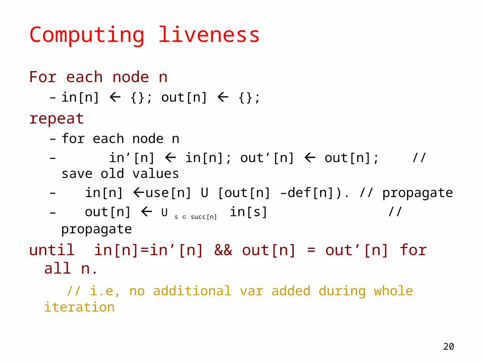
Computing liveness

For each node n– in[n] {}; out[n] {};

repeat– for each node n– in’[n] in[n]; out’[n] out[n]; // save old

values– in[n] use[n] U [out[n] –def[n]). // propagate

– out[n] U s succ[n] in[s] // propagate

until in[n]=in’[n] && out[n] = out’[n] for all n.

// i.e, no additional var added during whole iteration

21

Algorithm: Example

• Compute live variables for each point:

a := b + cd := -ae := d + f

f := 2 * eb := d + e

e := e - 1

b := f + c

{b}

{c,e}

{b}

{c,f} {c,f}

{b,c,e,f}

{c,d,e,f}

{b,c,f}

{c,d,f}{a,c,f}

return b

return b

The Register Interference Graph

• Two temporaries that are live simultaneously cannot be allocated in the same register

• We construct an undirected graph– A node for each temporary

– An edge between t1 and t2 if they are live simultaneously at some point in the program

• This is the register interference graph (RIG)– Two temporaries can be allocated to the same register if there is

no edge connecting them

Register Interference Graph. Example.

• For our example:

a

f

e

d

c

b

• E.g., b and c cannot be in the same register

• E.g., b and d can be in the same register

Register Interference Graph. Properties.

• It extracts exactly the information needed to characterize legal register assignments

• It gives a global (i.e., over the entire flow graph) picture of the register requirements

• After RIG construction the register allocation algorithm is architecture independent

Graph Coloring. Definitions.

• A coloring of a graph is an assignment of colors to nodes, such that nodes connected by an edge have different colors

• A graph is k-colorable if it has a coloring with k colors

Register Allocation Through Graph Coloring

• In our problem, colors = registers– We need to assign colors (registers) to graph nodes

(temporaries)

• Let k = number of machine registers

• If the RIG is k-colorable then there is a register assignment that uses no more than k registers

Graph Coloring. Example.

• Consider the example RIG

a

f

e

d

c

b

• There is no coloring with less than 4 colors• There are 4-colorings of this graph

r4

r1

r2

r3

r2

r3

Graph Coloring. Example.

• Under this coloring the code becomes:

r2 := r3 + r4

r3 := -r2

r2 := r3 + r1

r1 := 2 * r2

r3 := r3 + r2

r2 := r2 - 1

r3 := r1 + r4

Computing Graph Colorings

• The remaining problem is to compute a coloring for the interference graph

• But:1. This problem is very hard (NP-hard). No efficient algorithms are

known.

2. A coloring might not exist for a given number or registers

• The solution to (1) is to use heuristics• We’ll consider later the other problem

Graph Coloring Heuristic

• Observation:– Pick a node t with fewer than k neighbors in RIG– Eliminate t and its edges from RIG– If the resulting graph has a k-coloring then so does the original

graph

• Why:– Let c1,…,cn be the colors assigned to the neighbors of t in the

reduced graph– Since n < k we can pick some color for t that is different from

those of its neighbors

Graph Coloring Heuristic

• The following works well in practice:– Pick a node t with fewer than k neighbors– Put t on a stack and remove it from the RIG– Repeat until the graph has one node

• Then start assigning colors to nodes on the stack (starting with the last node added)– At each step pick a color different from those assigned to already

colored neighbors

Graph Coloring Example (1)

• Remove a and then d

a

f

e

d

c

b

• Start with the RIG and with k = 4:

Stack: {}

Graph Coloring Example (2)

• Now all nodes have fewer than 4 neighbors and can be removed: c, b, e, f

f

e c

b

Stack: {d, a}

Graph Coloring Example (2)

• Start assigning colors to: f, e, b, c, d, a

b

a

e c r4

fr1

r2

r3

r2

r3

d

What if the Heuristic Fails?

• What if during simplification we get to a state where all nodes have k or more neighbors ?

• Example: try to find a 3-coloring of the RIG:

a

f

e

d

c

b

What if the Heuristic Fails?

• Remove a and get stuck (as shown below)

f

e

d

c

b

• Pick a node as a candidate for spilling– A spilled temporary “lives” in memory

• Assume that f is picked as a candidate

What if the Heuristic Fails?

• Remove f and continue the simplification– Simplification now succeeds: b, d, e, c

e

d

c

b

What if the Heuristic Fails?

• On the assignment phase we get to the point when we have to assign a color to f

• We hope that among the 4 neighbors of f we use less than 3 colors optimistic coloring

f

e

d

c

b r3

r1r2

r3

?

Spilling

• Since optimistic coloring failed we must spill temporary f• We must allocate a memory location as the home of f

– Typically this is in the current stack frame – Call this address fa

• Before each operation that uses f, insert f := load fa

• After each operation that defines f, insert store f, fa

Spilling. Example.

• This is the new code after spilling f

a := b + cd := -af := load fae := d + f

f := 2 * estore f, fa

b := d + e

e := e - 1

f := load fab := f + c

Recomputing Liveness Information

• The new liveness information after spilling:

a := b + cd := -af := load fae := d + f

f := 2 * estore f, fa

b := d + e

e := e - 1

f := load fab := f + c

{b}

{c,e}

{b}

{c,f}{c,f}

{b,c,e,f}

{c,d,e,f}

{b,c,f}

{c,d,f}{a,c,f}

{c,d,f}

{c,f}

{c,f}

Recomputing Liveness Information

• The new liveness information is almost as before• f is live only

– Between a f := load fa and the next instruction– Between a store f, fa and the preceding instr.

• Spilling reduces the live range of f• And thus reduces its interferences• Which result in fewer neighbors in RIG for f

Recompute RIG After Spilling

• The only changes are in removing some of the edges of the spilled node

• In our case f still interferes only with c and d• And the resulting RIG is 3-colorable

a

f

e

d

c

b

Spilling (Cont.)

• Additional spills might be required before a coloring is found

• The tricky part is deciding what to spill• Possible heuristics:

– Spill temporaries with most conflicts– Spill temporaries with few definitions and uses– Avoid spilling in inner loops

• Any heuristic is correct

Conclusions

• Register allocation is a “must have” optimization in most compilers:– Because intermediate code uses too many temporaries– Because it makes a big difference in performance

• Graph coloring is a powerful register allocation schemes• Register allocation is more complicated for CISC

machines