1 linear functions straight lines and · are familiar with the rules governing these algebraic...
TRANSCRIPT
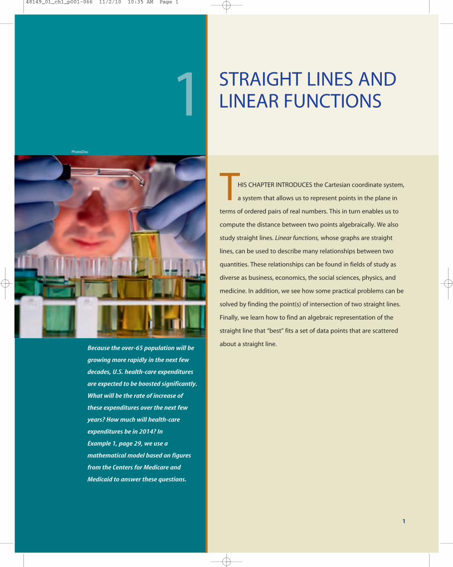
Because the over-65 population will be
growing more rapidly in the next few
decades, U.S. health-care expenditures
are expected to be boosted significantly.
What will be the rate of increase of
these expenditures over the next few
years? How much will health-care
expenditures be in 2014? In
Example 1, page 29, we use a
mathematical model based on figures
from the Centers for Medicare and
Medicaid to answer these questions.
THIS CHAPTER INTRODUCES the Cartesian coordinate system,
a system that allows us to represent points in the plane in
terms of ordered pairs of real numbers. This in turn enables us to
compute the distance between two points algebraically. We also
study straight lines. Linear functions, whose graphs are straight
lines, can be used to describe many relationships between two
quantities. These relationships can be found in fields of study as
diverse as business, economics, the social sciences, physics, and
medicine. In addition, we see how some practical problems can be
solved by finding the point(s) of intersection of two straight lines.
Finally, we learn how to find an algebraic representation of the
straight line that “best” fits a set of data points that are scattered
about a straight line.
STRAIGHT LINES ANDLINEAR FUNCTIONS1
PhotoDisc
1
48149_01_ch1_p001-066 11/2/10 10:35 AM Page 1
2 CHAPTER 1 STRAIGHT LINES AND LINEAR FUNCTIONS
The Cartesian Coordinate System
The real number system is made up of the set of real numbers together with the usualoperations of addition, subtraction, multiplication, and division. We assume that youare familiar with the rules governing these algebraic operations (see Appendix B).
Real numbers may be represented geometrically by points on a line. This line iscalled the real number, or coordinate, line. We can construct the real number line asfollows: Arbitrarily select a point on a straight line to represent the number 0. Thispoint is called the origin. If the line is horizontal, then choose a point at a convenientdistance to the right of the origin to represent the number 1. This determines the scalefor the number line. Each positive real number x lies x units to the right of 0, and eachnegative real number x lies �x units to the left of 0.
In this manner, a one-to-one correspondence is set up between the set of real num-bers and the set of points on the number line, with all the positive numbers lying to theright of the origin and all the negative numbers lying to the left of the origin (Figure 1).
In a similar manner, we can represent points in a plane (a two-dimensional space)by using the Cartesian coordinate system, which we construct as follows: Take twoperpendicular lines, one of which is normally chosen to be horizontal. These linesintersect at a point O, called the origin (Figure 2). The horizontal line is called the x-axis, and the vertical line is called the y-axis. A number scale is set up along the x-axis, with the positive numbers lying to the right of the origin and the negative num-bers lying to the left of it. Similarly, a number scale is set up along the y-axis, with thepositive numbers lying above the origin and the negative numbers lying below it.
Note The number scales on the two axes need not be the same. Indeed, in manyapplications, different quantities are represented by x and y. For example, x may rep-resent the number of cell phones sold, and y may represent the total revenue resultingfrom the sales. In such cases, it is often desirable to choose different number scales torepresent the different quantities. Note, however, that the zeros of both number scalescoincide at the origin of the two-dimensional coordinate system.
We can represent a point in the plane that is uniquely in this coordinate system byan ordered pair of numbers—that is, a pair (x, y) in which x is the first number andy is the second. To see this, let P be any point in the plane (Figure 3). Draw perpen-dicular lines from P to the x-axis and y-axis, respectively. Then the number x is pre-cisely the number that corresponds to the point on the x-axis at which the perpendic-ular line through P hits the x-axis. Similarly, y is the number that corresponds to thepoint on the y-axis at which the perpendicular line through P crosses the y-axis.
Conversely, given an ordered pair (x, y) with x as the first number and y as thesecond, a point P in the plane is uniquely determined as follows: Locate the point onthe x-axis represented by the number x, and draw a line through that point perpendic-ular to the x-axis. Next, locate the point on the y-axis represented by the number y, anddraw a line through that point perpendicular to the y-axis. The point of intersection ofthese two lines is the point P (Figure 3).
– 4 – 3 – 2 – 1 10 2 3 4
Origin
x
122– 3
FIGURE 1The real number line
xO x-axis
y
y-axis Origin
FIGURE 2The Cartesian coordinate system
xO x
y
y P(x, y)
FIGURE 3An ordered pair in the coordinate plane
1.1 The Cartesian Coordinate System
48149_01_ch1_p001-066 11/2/10 10:35 AM Page 2

In the ordered pair (x, y), x is called the abscissa, or x-coordinate; y is called theordinate, or y-coordinate; and x and y together are referred to as the coordinates ofthe point P. The point P with x-coordinate equal to a and y-coordinate equal to b isoften written P(a, b).
The points A(2, 3), B(�2, 3), C(�2, �3), D(2, �3), E(3, 2), F(4, 0), and G(0, �5) are plotted in Figure 4.
Note In general, (x, y) � (y, x). This is illustrated by the points A and E in Figure 4.
The axes divide the plane into four quadrants. Quadrant I consists of the points P withcoordinates x and y, denoted by P(x, y), satisfying x � 0 and y � 0; Quadrant II con-sists of the points P(x, y) where x � 0 and y � 0; Quadrant III consists of the pointsP(x, y) where x � 0 and y � 0; and Quadrant IV consists of the points P(x, y) wherex � 0 and y � 0 (Figure 5).
The Distance Formula
One immediate benefit that arises from using the Cartesian coordinate system is thatthe distance between any two points in the plane may be expressed solely in terms ofthe coordinates of the points. Suppose, for example, (x1, y1) and (x2, y2) are any twopoints in the plane (Figure 6). Then we have the following:
For a proof of this result, see Exercise 46, page 8.
xO
Quadrant I (+, +)
y
Quadrant II (–, +)
Quadrant III (–, –)
Quadrant IV (+, –)
x1 3 5
y
4
2
B(–2, 3) A(2, 3)
–3 –1
D(2, –3)C(–2, –3)
–2
–4
–6
F(4, 0)
E(3, 2)
G(0, –5)
1.1 THE CARTESIAN COORDINATE SYSTEM 3
FIGURE 4Several points in the coordinate plane
FIGURE 5The four quadrants in the coordinateplane
Distance Formula
The distance d between two points P1 1x1, y1 2 and P2 1x2, y2 2 in the plane is given by
(1)d � 21x2 � x1 2 2 � 1 y2 � y1 2 2FIGURE 6The distance between two points in thecoordinate plane
x
y
d
P1(x1, y1)
P2(x2, y2)
48149_01_ch1_p001-066 11/2/10 10:35 AM Page 3

In what follows, we give several applications of the distance formula.
EXAMPLE 1 Find the distance between the points (�4, 3) and (2, 6).
Solution Let P1(�4, 3) and P2(2, 6) be points in the plane. Then we have
x1 � �4 and y1 � 3
x2 � 2 y2 � 6
Using Formula (1), we have
APPLIED EXAMPLE 2 The Cost of Laying Cable In Figure 7, S representsthe position of a power relay station located on a straight coastal highway,
and M shows the location of a marine biology experimental station on a nearbyisland. A cable is to be laid connecting the relay station at S with the experimentalstation at M via the point Q that lies on the x-axis between O and S. If the cost ofrunning the cable on land is $3 per running foot and the cost of running the cableunderwater is $5 per running foot, find the total cost for laying the cable.
Solution The length of cable required on land is given by the distance from S toQ. This distance is (10,000 � 2000), or 8000 feet. Next, we see that the length ofcable required underwater is given by the distance from Q to M. This distance is
or approximately 3606 feet. Therefore, the total cost for laying the cable is approx-imately
3(8000) � 5(3606) � 42,030
dollars.
EXAMPLE 3 Let P(x, y) denote a point lying on a circle with radius r and centerC(h, k) (Figure 8). Find a relationship between x and y.
Solution By the definition of a circle, the distance between C(h, k) and P(x, y) is r. Using Formula (1), we have
21x � h 2 2 � 1 y � k 2 2 � r
� 3606
� 113,000,000
210 � 2000 2 2 � 13000 � 0 2 2 � 220002 � 30002
x (feet)O S(10,000, 0) Q(2000, 0)
y (feet)
M(0, 3000)(0, 3000)M(0, 3000)
� 315
� 145
� 262 � 32
d � 2 32 � 1�4 2 4 2 � 16 � 3 2 2
4 CHAPTER 1 STRAIGHT LINES AND LINEAR FUNCTIONS
FIGURE 7The cable will connect the relay station Sto the experimental station M.
Explore & DiscussRefer to Example 1. Supposewe label the point (2, 6) asP1 and the point (�4, 3) asP2. (1) Show that the dis-tance d between the twopoints is the same as thatobtained earlier. (2) Provethat, in general, the distanced in Formula (1) is indepen-dent of the way we label thetwo points.
VIDEO
48149_01_ch1_p001-066 11/2/10 10:35 AM Page 4
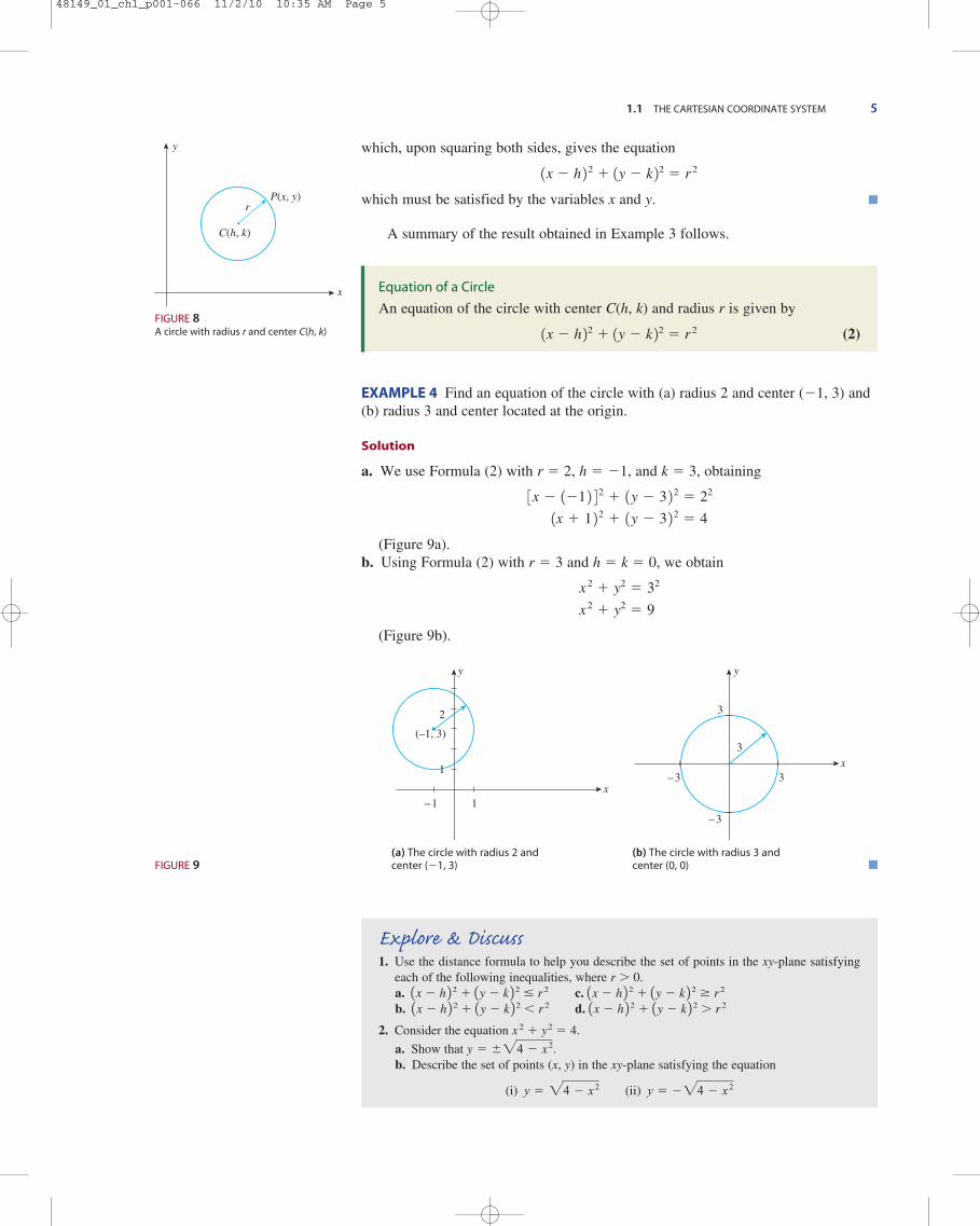
which, upon squaring both sides, gives the equation
1x � h 22 � 1y � k 22 � r2
which must be satisfied by the variables x and y.
A summary of the result obtained in Example 3 follows.
EXAMPLE 4 Find an equation of the circle with (a) radius 2 and center (�1, 3) and(b) radius 3 and center located at the origin.
Solution
a. We use Formula (2) with r � 2, h � �1, and k � 3, obtaining
(Figure 9a).b. Using Formula (2) with r � 3 and h � k � 0, we obtain
(Figure 9b).
(a) The circle with radius 2 and (b) The circle with radius 3 and center (�1, 3) center (0, 0)
x
y
–1 1
2
(–1, 3)
x
y
3
13–3
3
–3
x 2 � y2 � 9
x 2 � y2 � 32
1x � 1 2 2 � 1 y � 3 2 2 � 4
3x � 1�1 2 4 2 � 1 y � 3 2 2 � 22
Equation of a Circle
An equation of the circle with center C(h, k) and radius r is given by
1x � h 22 � 1y � k 22 � r2 (2)
1.1 THE CARTESIAN COORDINATE SYSTEM 5
x
y
C(h, k)
rP(x, y)
FIGURE 8A circle with radius r and center C(h, k)
FIGURE 9
Explore & Discuss1. Use the distance formula to help you describe the set of points in the xy-plane satisfying
each of the following inequalities, where r � 0.a. 1x � h 2 2 � 1y � k 2 2 � r2 c. 1x � h 2 2 � 1y � k 2 2 r2
b. 1x � h 2 2 � 1y � k 2 2 � r2 d. 1x � h 2 2 � 1y � k 2 2 � r2
2. Consider the equation x2 � y2 � 4.
a. Show that b. Describe the set of points (x, y) in the xy-plane satisfying the equation
(i) (ii) y � �24 � x 2y � 24 � x
2
y � 24 � x 2.
48149_01_ch1_p001-066 11/2/10 10:35 AM Page 5

6 CHAPTER 1 STRAIGHT LINES AND LINEAR FUNCTIONS
1. a. Plot the points A(4, �2), B(2, 3), and C(�3, 1).b. Find the distance between the points A and B, between
B and C, and between A and C.c. Use the Pythagorean Theorem to show that the triangle
with vertices A, B, and C is a right triangle.
2. The accompanying figure shows the location of Cities A, B,and C. Suppose a pilot wishes to fly from City A to City Cbut must make a mandatory stopover in City B. If the sin-
1. What can you say about the signs of a and b if the point P(a, b) lies in (a) the second quadrant? (b) The thirdquadrant? (c) The fourth quadrant?
2. a. What is the distance between P1(x1, y1) and P2(x2, y2)?b. When you use the distance formula, does it matter
which point is labeled P1 and which point is labeledP2? Explain.
x (miles)100 200 300 400 500 600 700
y (miles)
300
200
100
B(200, 50)
A(0, 0)
C(600, 320)
Solutions to Self-Check Exercises 1.1 can be found on page 9.
1.1 Exercises
1.1 Self-Check Exercises
1.1 Concept Questions
gle-engine light plane has a range of 650 mi, can the pilotmake the trip without refueling in City B?
In Exercises 1–6, refer to the accompanying figure and deter-mine the coordinates of the point and the quadrant in which it islocated.
1. A 2. B 3. C
4. D 5. E 6. F
x1 3 5 7 9
y
3
1
BA
–5 –3 –1
D
C–3
–5
–7
F
E
In Exercises 7–12, refer to the accompanying figure.
7. Which point has coordinates (4, 2)?
8. What are the coordinates of point B?
9. Which points have negative y-coordinates?
10. Which point has a negative x-coordinate and a negative y-coordinate?
11. Which point has an x-coordinate that is equal to zero?
12. Which point has a y-coordinate that is equal to zero?
2 4 6x
y
4
2
B
A
–6 –4 –2
D
G–2
–4
FE
C
48149_01_ch1_p001-066 11/2/10 10:35 AM Page 6

1.1 THE CARTESIAN COORDINATE SYSTEM 7
In Exercises 13–20, sketch a set of coordinate axes and then plotthe point.
13. (�2, 5) 14. (1, 3)
15. (3, �1) 16. (3, �4)
17. 18, � 2 18. 1� , 219. (4.5, �4.5) 20. (1.2, �3.4)
In Exercises 21–24, find the distance between the points.
21. (1, 3) and (4, 7) 22. (1, 0) and (4, 4)
23. (�1, 3) and (4, 9)
24. (�2, 1) and (10, 6)
25. Find the coordinates of the points that are 10 units awayfrom the origin and have a y-coordinate equal to �6.
26. Find the coordinates of the points that are 5 units awayfrom the origin and have an x-coordinate equal to 3.
27. Show that the points (3, 4), (�3, 7), (�6, 1), and (0, �2)form the vertices of a square.
28. Show that the triangle with vertices (�5, 2), (�2, 5), and(5, �2) is a right triangle.
In Exercises 29–34, find an equation of the circle that satisfies thegiven conditions.
29. Radius 5 and center (2, �3)
30. Radius 3 and center (�2, �4)
31. Radius 5 and center at the origin
32. Center at the origin and passes through (2, 3)
33. Center (2, �3) and passes through (5, 2)
34. Center (�a, a) and radius 2a
35. DISTANCE TRAVELED A grand tour of four cities begins at CityA and makes successive stops at Cities B, C, and D beforereturning to City A. If the cities are located as shown in theaccompanying figure, find the total distance covered on thetour.
x (miles)500
y (miles)
500
B (400, 300)
A(0, 0)–500
D (–800, 0)
C (–800, 800)
32
52
72
36. DELIVERY CHARGES A furniture store offers free setup anddelivery services to all points within a 25-mi radius of itswarehouse distribution center. If you live 20 mi east and14 mi south of the warehouse, will you incur a deliverycharge? Justify your answer.
37. OPTIMIZING TRAVEL TIME Towns A, B, C, and D are locatedas shown in the accompanying figure. Two highways linkTown A to Town D. Route 1 runs from Town A to Town Dvia Town B, and Route 2 runs from Town A to Town D viaTown C. If a salesman wishes to drive from Town A toTown D and traffic conditions are such that he couldexpect to average the same speed on either route, whichhighway should he take to arrive in the shortest time?
38. MINIMIZING SHIPPING COSTS Refer to the figure for Exercise37. Suppose a fleet of 100 automobiles are to be shippedfrom an assembly plant in Town A to Town D. They maybe shipped either by freight train along Route 1 at a costof 66¢/mile/automobile or by truck along Route 2 at a costof 62¢/mile/automobile. Which means of transportationminimizes the shipping cost? What is the net savings?
39. CONSUMER DECISIONS Will Barclay wishes to determinewhich HDTV antenna he should purchase for his home. TheTV store has supplied him with the following information:
Range in miles
VHF UHF Model Price
30 20 A $50
45 35 B 60
60 40 C 70
75 55 D 80
Will wishes to receive Channel 17 (VHF), which is located25 mi east and 35 mi north of his home, and Channel 38(UHF), which is located 20 mi south and 32 mi west of hishome. Which model will allow him to receive both chan-nels at the least cost? (Assume that the terrain betweenWill’s home and both broadcasting stations is flat.)
40. COST OF LAYING CABLE In the accompanying diagram, S rep-resents the position of a power relay station located on astraight coastal highway, and M shows the location of amarine biology experimental station on a nearby island. A
x (miles)1000
y (miles)
1000
B (400, 300)
A (0, 0)
D(1300, 1500)C(800, 1500)
12
48149_01_ch1_p001-066 11/2/10 10:35 AM Page 7

8 CHAPTER 1 STRAIGHT LINES AND LINEAR FUNCTIONS
cable is to be laid connecting the relay station at S with theexperimental station at M via the point Q that lies on the x-axis between O and S. If the cost of running the cable onland is $3/running foot and the cost of running cable under-water is $5/running foot, find an expression in terms of x thatgives the total cost of laying the cable. Use this expressionto find the total cost when x � 1500 and when x � 2500.
41. DISTANCE BETWEEN SHIPS Two ships leave port at the sametime. Ship A sails north at a speed of 20 mph while Ship Bsails east at a speed of 30 mph.a. Find an expression in terms of the time t (in hours) giv-
ing the distance between the two ships.b. Using the expression obtained in part (a), find the dis-
tance between the two ships 2 hr after leaving port.
42. DISTANCE BETWEEN SHIPS Sailing north at a speed of 25 mph, Ship A leaves a port. A half hour later, Ship Bleaves the same port, sailing east at a speed of 20 mph. Lett (in hours) denote the time Ship B has been at sea.a. Find an expression in terms of t that gives the distance
between the two ships.b. Use the expression obtained in part (a) to find the distance
between the two ships 2 hr after Ship A has left the port.
43. WATCHING A ROCKET LAUNCH At a distance of 4000 ft fromthe launch site, a spectator is observing a rocket beinglaunched. Suppose the rocket lifts off vertically and reachesan altitude of x feet, as shown below:
a. Find an expression giving the distance between thespectator and the rocket.
b. What is the distance between the spectator and the rocketwhen the rocket reaches an altitude of 20,000 ft?
x
4000 ft
Rocket
Launching padSpectator
x (feet)O S(10,000, 0) Q(x, 0)
y (feet)
M(0, 3000)(0, 3000)M(0, 3000)
In Exercises 44 and 45, determine whether the statement is trueor false. If it is true, explain why it is true. If it is false, give anexample to show why it is false.
44. If the distance between the points P1(a, b) and P2(c, d ) is D, then the distance between the points P1(a, b) andP3(kc, kd ) (k � 0) is given by D.
45. The circle with equation kx2 � ky2 � a2 lies inside the cir-cle with equation x2 � y2 � a2, provided that k � 1 and a � 0.
46. Let 1x1, y1 2 and 1x2, y2 2 be two points lying in the xy-plane.Show that the distance between the two points is given by
Hint: Refer to the accompanying figure, and use the PythagoreanTheorem.
47. a. Show that the midpoint of the line segment joining thepoints P1 1x1, y1 2 and P2 1x2, y2 2 is
b. Use the result of part (a) to find the midpoint of the linesegment joining the points (�3, 2) and (4, �5).
48. In the Cartesian coordinate system, the two axes are per-pendicular to each other. Consider a coordinate system inwhich the x-axis and y-axis are noncollinear (that is, theaxes do not lie along a straight line) and are not perpendic-ular to each other (see the accompanying figure).a. Describe how a point is represented in this coordinate
system by an ordered pair (x, y) of real numbers. Con-versely, show how an ordered pair (x, y) of real numbersuniquely determines a point in the plane.
b. Suppose you want to find a formula for the distancebetween two points, P1 1x1, y1 2 and P2 1x2, y2 2 , in theplane. What advantage does the Cartesian coordinate sys-tem have over the coordinate system under consideration?
x
y
O
a x1 � x2
2,
y1 � y2
2b
y
x
y2 – y1
x2 – x1
(x1, y1)
(x2, y2)
d � 21x2 � x1 2 2 � 1 y2 � y1 2 2
0 k 0
48149_01_ch1_p001-066 11/2/10 10:35 AM Page 8

1. a. The points are plotted in the following figure.
b. The distance between A and B is
The distance between B and C is
� 21�5 2 2 � 1�2 2 2 � 125 � 4 � 129
d1B, C 2 � 21�3 � 2 2 2 � 11 � 3 2 2
� 21�2 2 2 � 52 � 14 � 25 � 129
d1A, B 2 � 212 � 4 2 2 � 33 � 1�2 2 4 2
x5
y
5
B(2, 3)
–5
–5
A(4, –2)
C(– 3, 1)
1.2 STRAIGHT LINES 9
The distance between A and C is
c. We will show that
[d(A, C)]2 � [d(A, B)]2 � [d(B, C )]2
From part (b), we see that 3d 1A, B 242 � 29, 3d 1B, C 242� 29, and 3d 1A, C 24 2 � 58, and the desired result fol-lows.
2. The distance between City A and City B is
or 206 mi. The distance between City B and City C is
or 483 mi. Therefore, the total distance the pilot wouldhave to cover is 689 mi, so she must refuel in City B.
� 2400 2 � 270
2 � 483
d1B, C 2 � 21600 � 200 2 2 � 1320 � 50 2 2
d1A, B 2 � 2200 2 � 50
2 � 206
� 21�7 2 2 � 32 � 149 � 9 � 158
d1A, C 2 � 21�3 � 4 2 2 � 31 � 1�2 2 4 2
1.1 Solutions to Self-Check Exercises
1.2 Straight Lines
In computing income tax, business firms are allowed by law to depreciate certainassets such as buildings, machines, furniture, and automobiles over a period of time.Linear depreciation, or the straight-line method, is often used for this purpose. Thegraph of the straight line shown in Figure 10 describes the book value V of a networkserver that has an initial value of $10,000 and that is being depreciated linearly over5 years with a scrap value of $3000. Note that only the solid portion of the straight lineis of interest here.
The book value of the server at the end of year t, where t lies between 0 and 5,can be read directly from the graph. But there is one shortcoming in this approach: Theresult depends on how accurately you draw and read the graph. A better and moreaccurate method is based on finding an algebraic representation of the depreciationline. (We continue our discussion of the linear depreciation problem in Section 1.3.)
t1 2 3 4 5
V ($)
10,000
3000
Years
(5, 3000)
FIGURE 10Linear depreciation of an asset
48149_01_ch1_p001-066 11/2/10 10:35 AM Page 9

To see how a straight line in the xy-plane may be described algebraically, we needfirst to recall certain properties of straight lines.
Slope of a Line
Let L denote the unique straight line that passes through the two distinct points 1x1, y1 2 and 1x2, y2 2. If x1 � x2, then we define the slope of L as follows.
If x1 � x2, then L is a vertical line (Figure 12). Its slope is undefined since the denom-inator in Equation (3) will be zero and division by zero is proscribed.
Observe that the slope of a straight line is a constant whenever it is defined. Thenumber �y � y2 � y1 (�y is read “delta y”) is a measure of the vertical change in y,and �x � x2 � x1 is a measure of the horizontal change in x as shown in Figure 11.From this figure we can see that the slope m of a straight line L is a measure of therate of change of y with respect to x. Furthermore, the slope of a nonvertical straightline is constant, and this tells us that this rate of change is constant.
Figure 13a shows a straight line L1 with slope 2. Observe that L1 has the propertythat a 1-unit increase in x results in a 2-unit increase in y. To see this, let �x � 1 in
(a) The line rises (m � 0). (b) The line falls (m � 0).
10 CHAPTER 1 STRAIGHT LINES AND LINEAR FUNCTIONS
y
x
(x1, y1 )
(x2, y 2)
L
FIGURE 12The slope is undefined if x1 � x2.
FIGURE 13
y
x
L1
y
x
1
2m = 2
L2
1 m = –1
–1
Slope of a Nonvertical Line
If 1x1, y1 2 and 1x2, y2 2 are any two distinct points on a nonvertical line L, then theslope m of L is given by
(3)
(Figure 11).
m �¢y
¢x�
y2 � y1
x2 � x1
y
x
(x1, y1)
(x2, y2)
L
y2 – y1 = Δy
x2 – x1 = Δ x
FIGURE 11
48149_01_ch1_p001-066 11/2/10 10:35 AM Page 10
Equation (3) so that m � �y. Since m � 2, we conclude that �y � 2. Similarly, Fig-ure 13b shows a line L2 with slope �1. Observe that a straight line with positive slopeslants upward from left to right (y increases as x increases), whereas a line with neg-ative slope slants downward from left to right (y decreases as x increases). Finally,Figure 14 shows a family of straight lines passing through the origin with indicatedslopes.
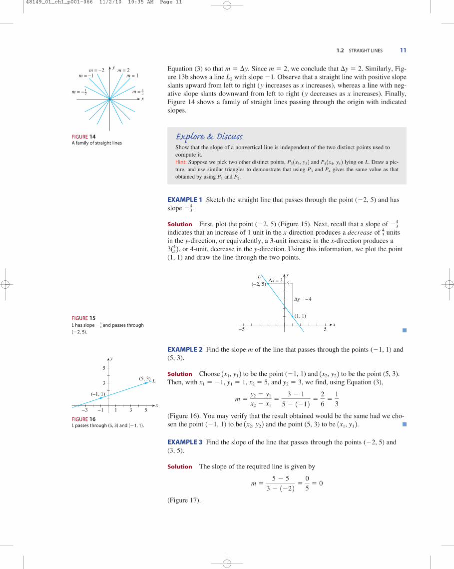
EXAMPLE 1 Sketch the straight line that passes through the point (�2, 5) and hasslope .
Solution First, plot the point (�2, 5) (Figure 15). Next, recall that a slope of indicates that an increase of 1 unit in the x-direction produces a decrease of unitsin the y-direction, or equivalently, a 3-unit increase in the x-direction produces a
, or 4-unit, decrease in the y-direction. Using this information, we plot the point(1, 1) and draw the line through the two points.
EXAMPLE 2 Find the slope m of the line that passes through the points (�1, 1) and(5, 3).
Solution Choose 1x1, y1 2 to be the point (�1, 1) and 1x2, y2 2 to be the point (5, 3).Then, with x1 � �1, y1 � 1, x2 � 5, and y2 � 3, we find, using Equation (3),
(Figure 16). You may verify that the result obtained would be the same had we cho-sen the point (�1, 1) to be 1x2, y2 2 and the point (5, 3) to be 1x1, y1 2.EXAMPLE 3 Find the slope of the line that passes through the points (�2, 5) and (3, 5).
Solution The slope of the required line is given by
(Figure 17).
m �5 � 5
3 � 1�2 2 �0
5� 0
m �y2 � y1
x2 � x1�
3 � 1
5 � 1�1 2 �2
6�
1
3
x
yL
(1, 1)
(–2, 5)
Δy = –4
Δx = 3
5–5
5
3143 243
�43
�43
1.2 STRAIGHT LINES 11
y
x
m = 2m = 1
m = –2m = –1
m = – 12
m = 12
FIGURE 14A family of straight lines
FIGURE 15L has slope and passes through
(�2, 5).
�43
Explore & DiscussShow that the slope of a nonvertical line is independent of the two distinct points used tocompute it.Hint: Suppose we pick two other distinct points, P3 1x3, y3 2 and P4 1x4, y4 2 lying on L. Draw a pic-ture, and use similar triangles to demonstrate that using P3 and P4 gives the same value as thatobtained by using P1 and P2.
x
y
L
1 3 5–3 –1
5
3(5, 3)
(–1, 1)
FIGURE 16L passes through (5, 3) and (�1, 1).
48149_01_ch1_p001-066 11/2/10 10:35 AM Page 11
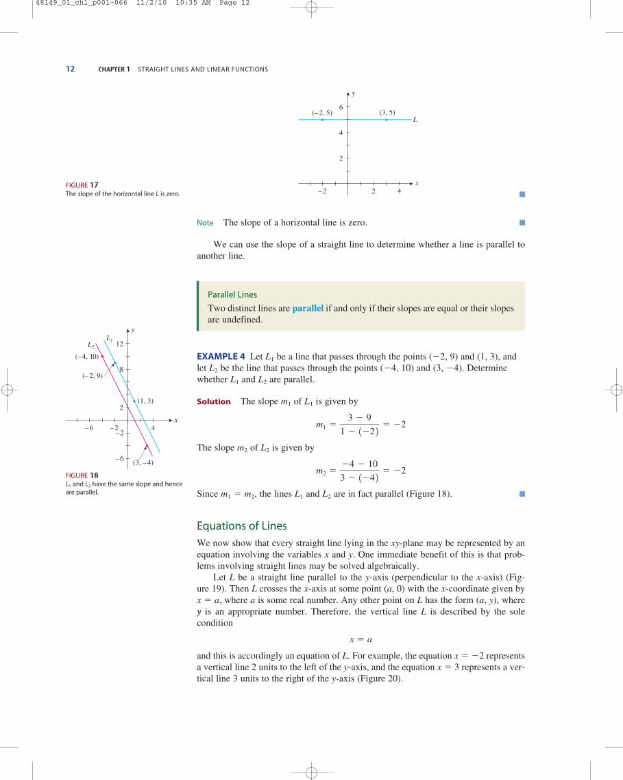
12 CHAPTER 1 STRAIGHT LINES AND LINEAR FUNCTIONS
Note The slope of a horizontal line is zero.
We can use the slope of a straight line to determine whether a line is parallel toanother line.
EXAMPLE 4 Let L1 be a line that passes through the points (�2, 9) and (1, 3), andlet L2 be the line that passes through the points (�4, 10) and (3, �4). Determinewhether L1 and L2 are parallel.
Solution The slope m1 of L1 is given by
The slope m2 of L2 is given by
Since m1 � m2, the lines L1 and L2 are in fact parallel (Figure 18).
Equations of Lines
We now show that every straight line lying in the xy-plane may be represented by anequation involving the variables x and y. One immediate benefit of this is that prob-lems involving straight lines may be solved algebraically.
Let L be a straight line parallel to the y-axis (perpendicular to the x-axis) (Fig-ure 19). Then L crosses the x-axis at some point (a, 0) with the x-coordinate given byx � a, where a is some real number. Any other point on L has the form (a, y), whereyy is an appropriate number. Therefore, the vertical line L is described by the sole condition
x � a
and this is accordingly an equation of L. For example, the equation x � �2 representsa vertical line 2 units to the left of the y-axis, and the equation x � 3 represents a ver-tical line 3 units to the right of the y-axis (Figure 20).
m2 ��4 � 10
3 � 1�4 2 � �2
m1 �3 � 9
1 � 1�2 2 � �2
Parallel Lines
Two distinct lines are parallel if and only if their slopes are equal or their slopesare undefined.
x
y
(–2, 5)L
(3, 5)
2 4–2
6
4
2
FIGURE 17The slope of the horizontal line L is zero.
x
y
(–2, 9)
L1
(1, 3)
4–2
12
8
2
–6
(–4, 10)
(3, –4)
–2
–6
L2
FIGURE 18L1 and L2 have the same slope and henceare parallel.
48149_01_ch1_p001-066 11/2/10 10:35 AM Page 12

1.2 STRAIGHT LINES 13
Next, suppose L is a nonvertical line, so it has a well-defined slope m. Suppose(x1, y1) is a fixed point lying on L and (x, y) is a variable point on L distinct from (x1, y1) (Figure 21). Using Equation (3) with the point (x2, y2) � (x, y), we findthat the slope of L is given by
Upon multiplying both sides of the equation by x � x1, we obtain Equation (4).
Equation (4) is called the point-slope form of an equation of a line because it uses agiven point 1x1, y1 2 on a line and the slope m of the line.
EXAMPLE 5 Find an equation of the line that passes through the point (1, 3) andhas slope 2.
Solution Using the point-slope form of the equation of a line with the point (1, 3)and m � 2, we obtain
y � 3 � 2 1x � 1 2 y � y1 � m(x � x1)
which, when simplified, becomes
2x � y � 1 � 0
(Figure 22).
Point-Slope Form of an Equation of a Line
An equation of the line that has slope m and passes through the point (x1, y1) isgiven by
y � y1 � m 1x � x1 2 (4)
m �y � y1
x � x1
FIGURE 19The vertical line x � a
y
x
(a, y)
(a, 0)
L
FIGURE 20The vertical lines x � �2 and x � 3
FIGURE 21L passes through (x1, y1) and has slope m.
y
x
(x1 y1, )
(x, y)
L
x
y
1 5–3 –1
5
3
1
x = –2 x = 3
x
yL
(1, 3)
2–2
4
2
FIGURE 22L passes through (1, 3) and has slope 2.
48149_01_ch1_p001-066 11/2/10 10:35 AM Page 13

EXAMPLE 6 Find an equation of the line that passes through the points (�3, 2) and(4, �1).
Solution The slope of the line is given by
Using the point-slope form of the equation of a line with the point (4, �1) and theslope , we have
y � y1 � m(x � x1)
(Figure 23).
We can use the slope of a straight line to determine whether a line is perpendicular toanother line.
If the line L1 is vertical (so that its slope is undefined), then L1 is perpendicular toanother line, L2, if and only if L2 is horizontal (so that its slope is zero). For a proof ofthese results, see Exercise 92, page 22.
EXAMPLE 7 Find an equation of the line that passes through the point (3, 1) and isperpendicular to the line of Example 5.
Solution Since the slope of the line in Example 5 is 2, it follows that the slope ofthe required line is given by , the negative reciprocal of 2. Using the point-slope form of the equation of a line, we obtain
y � y1 � m (x � x1)
(Figure 24).
x � 2y � 5 � 0
2y � 2 � �x � 3
y � 1 � �1
2 1x � 3 2
m � �12
x
y
(–3, 2) L
(4, –1) 2 4–4 –2
4
2
–2
3x � 7y � 5 � 0
7y � 7 � �3x � 12
y � 1 � �3
7 1x � 4 2
m � �37
m ��1 � 2
4 � 1�3 2 � �3
7
14 CHAPTER 1 STRAIGHT LINES AND LINEAR FUNCTIONS
FIGURE 23L passes through (�3, 2) and (4, �1).
x
y
(1, 3)
L1
(3, 1)
1 3 5
5
1
L2
FIGURE 24L2 is perpendicular to L1 and passesthrough (3, 1).
Perpendicular Lines
If L1 and L2 are two distinct nonvertical lines that have slopes m1 and m2, respec-tively, then L1 is perpendicular to L2 (written L1 ⊥ L2) if and only if
m1 � �1
m2
VIDEO
48149_01_ch1_p001-066 11/2/10 10:35 AM Page 14
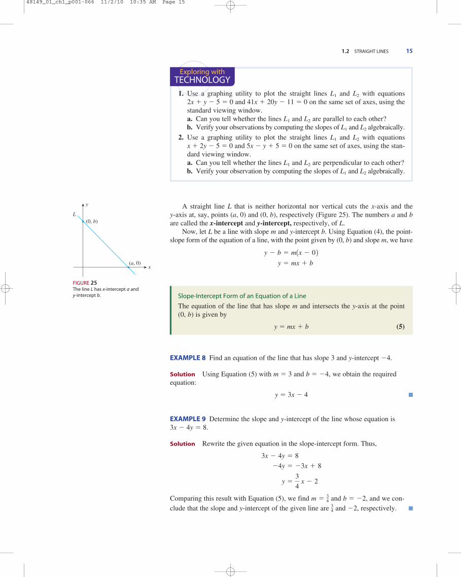
A straight line L that is neither horizontal nor vertical cuts the x-axis and the y-axis at, say, points (a, 0) and (0, b), respectively (Figure 25). The numbers a and bare called the x-intercept and y-intercept, respectively, of L.
Now, let L be a line with slope m and y-intercept b. Using Equation (4), the point-slope form of the equation of a line, with the point given by (0, b) and slope m, we have
EXAMPLE 8 Find an equation of the line that has slope 3 and y-intercept �4.
Solution Using Equation (5) with m � 3 and b � �4, we obtain the requiredequation:
y � 3x � 4
EXAMPLE 9 Determine the slope and y-intercept of the line whose equation is 3x � 4y � 8.
Solution Rewrite the given equation in the slope-intercept form. Thus,
Comparing this result with Equation (5), we find and b � �2, and we con-clude that the slope and y-intercept of the given line are and �2, respectively.3
4
m � 34
y �3
4 x � 2
�4y � �3x � 8
3x � 4y � 8
Slope-Intercept Form of an Equation of a Line
The equation of the line that has slope m and intersects the y-axis at the point (0, b) is given by
y � mx � b (5)
y � mx � b
y � b � m1x � 0 2
1.2 STRAIGHT LINES 15
x
y
(0, b)L
(a, 0)
FIGURE 25The line L has x-intercept a and y-intercept b.
Exploring withTECHNOLOGY
1. Use a graphing utility to plot the straight lines L1 and L2 with equations 2x � y � 5 � 0 and 41x � 20y � 11 � 0 on the same set of axes, using thestandard viewing window.a. Can you tell whether the lines L1 and L2 are parallel to each other?b. Verify your observations by computing the slopes of L1 and L2 algebraically.
2. Use a graphing utility to plot the straight lines L1 and L2 with equations x � 2y � 5 � 0 and 5x � y � 5 � 0 on the same set of axes, using the stan-dard viewing window.a. Can you tell whether the lines L1 and L2 are perpendicular to each other?b. Verify your observation by computing the slopes of L1 and L2 algebraically.
48149_01_ch1_p001-066 11/2/10 10:35 AM Page 15

APPLIED EXAMPLE 10 Sales of a Sporting Goods Store The sales managerof a local sporting goods store plotted sales versus time for the last 5 years
and found the points to lie approximately along a straight line (Figure 26). Byusing the points corresponding to the first and fifth years, find an equation of thetrend line. What sales figure can be predicted for the sixth year?
Solution Using Equation (3) with the points (1, 20) and (5, 60), we find that theslope of the required line is given by
Next, using the point-slope form of the equation of a line with the point (1, 20)and m � 10, we obtain
as the required equation.The sales figure for the sixth year is obtained by letting x � 6 in the last
equation, giving
y � 10 16 2 � 10 � 70
or $700,000.
APPLIED EXAMPLE 11 Appreciation in Value of an Art Object Suppose an art object purchased for $50,000 is expected to appreciate in value at a
constant rate of $5000 per year for the next 5 years. Use Equation (5) to write anequation predicting the value of the art object in the next several years. What willbe its value 3 years from the purchase date?
Solution Let x denote the time (in years) that has elapsed since the purchasedate and let y denote the object’s value (in dollars). Then, y � 50,000 when x � 0. Furthermore, the slope of the required equation is given by m � 5000,since each unit increase in x (1 year) implies an increase of 5000 units (dollars) in y. Using Equation (5) with m � 5000 and b � 50,000, we obtain
Three years from the purchase date, the value of the object will be given by
y � 5000(3) � 50,000
or $65,000.
y � mx � b y � 5000x � 50,000
y � 10 x � 10
y � y1 � m1 x � x1 2y � 20 � 101x � 1 2
m �60 � 20
5 � 1� 10
16 CHAPTER 1 STRAIGHT LINES AND LINEAR FUNCTIONS
x
y
1 2 3 4 5 6
70
60
50
40
30
20
10
Years
Sale
s in
ten
thou
sand
dol
lars
FIGURE 26Sales of a sporting goods store
Exploring withTECHNOLOGY
1. Use a graphing utility to plot the straight lines with equations y � �2x � 3,y � �x � 3, y � x � 3, and y � 2.5x � 3 on the same set of axes, using thestandard viewing window. What effect does changing the coefficient m of xin the equation y � mx � b have on its graph?
2. Use a graphing utility to plot the straight lines with equations y � 2x � 2, y � 2x � 1, y � 2x, y � 2x � 1, and y � 2x � 4 on the same set of axes,using the standard viewing window. What effect does changing the constantb in the equation y � mx � b have on its graph?
3. Describe in words the effect of changing both m and b in the equation y �mx � b.
Explore & DiscussRefer to Example 11. Can theequation predicting the value ofthe art object be used to predictlong-term growth?
VIDEO
48149_01_ch1_p001-066 11/2/10 10:35 AM Page 16
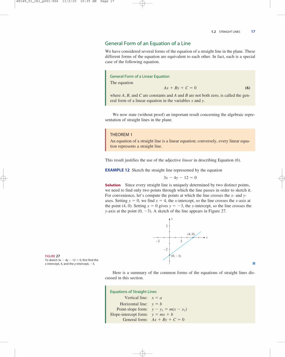
General Form of an Equation of a Line
We have considered several forms of the equation of a straight line in the plane. Thesedifferent forms of the equation are equivalent to each other. In fact, each is a specialcase of the following equation.
We now state (without proof) an important result concerning the algebraic repre-sentation of straight lines in the plane.
This result justifies the use of the adjective linear in describing Equation (6).
EXAMPLE 12 Sketch the straight line represented by the equation
3x � 4y � 12 � 0
Solution Since every straight line is uniquely determined by two distinct points,we need to find only two points through which the line passes in order to sketch it.For convenience, let’s compute the points at which the line crosses the x- and y-axes. Setting y � 0, we find x � 4, the x-intercept, so the line crosses the x-axis atthe point (4, 0). Setting x � 0 gives y � �3, the y-intercept, so the line crosses the y-axis at the point (0, �3). A sketch of the line appears in Figure 27.
Here is a summary of the common forms of the equations of straight lines dis-cussed in this section.
Equations of Straight Lines
Vertical line: x � a
Horizontal line: y � bPoint-slope form: y � y1 � m(x � x1)
Slope-intercept form: y � mx � bGeneral form: Ax � By � C � 0
x
y
(4, 0)
(0, – 3)
–2 2
2
–2
THEOREM 1
An equation of a straight line is a linear equation; conversely, every linear equa-tion represents a straight line.
General Form of a Linear Equation
The equationAx � By � C � 0 (6)
where A, B, and C are constants and A and B are not both zero, is called the gen-eral form of a linear equation in the variables x and y.
1.2 STRAIGHT LINES 17
FIGURE 27To sketch 3x � 4y � 12 � 0, first find thex-intercept, 4, and the y-intercept, �3.
48149_01_ch1_p001-066 11/2/10 10:35 AM Page 17

18 CHAPTER 1 STRAIGHT LINES AND LINEAR FUNCTIONS
1. Determine the number a such that the line passing throughthe points (a, 2) and (3, 6) is parallel to a line with slope 4.
2. Find an equation of the line that passes through the point (3, �1) and is perpendicular to a line with slope .
3. Does the point (3, �3) lie on the line with equation 2x � 3y � 12 � 0? Sketch the graph of the line.
4. SATELLITE TV SUBSCRIBERS The following table gives thenumber of satellite TV subscribers in the United States (inmillions) from 2004 through 2008 (t � 0 corresponds tothe beginning of 2004):
Year, t 0 1 2 3 4
Number, y 22.5 24.8 27.1 29.1 30.7
�12
In Exercises 1– 4, find the slope of the line shown in each figure.
1.
2.
x
y
2 4–2
4
2
–2
x
y
2–4 –2
4
–2
3.
4.
x
y
1 3– 3 – 1
5
3
1
x
y
2– 4 – 2
2
– 2
a. Plot the number of satellite TV subscribers in the UnitedStates (y) versus the year (t).
b. Draw the line L through the points (0, 22.5) and (4, 30.7).c. Find an equation of the line L.d. Assuming that this trend continues, estimate the number
of satellite TV subscribers in the United States in 2010.Sources: National Cable & Telecommunications Association and theFederal Communications Commission.
Solutions to Self-Check Exercises 1.2 can be found on page 23.
1.2 Exercises
1.2 Self-Check Exercises
1.2 Concept Questions
1. What is the slope of a nonvertical line? What can you sayabout the slope of a vertical line?
2. Give (a) the point-slope form, (b) the slope-intercept form,and (c) the general form of an equation of a line.
3. Let L1 have slope m1 and let L2 have slope m2. State theconditions on m1 and m2 if (a) L1 is parallel to L2 and (b) L1
is perpendicular to L2.
48149_01_ch1_p001-066 11/2/10 10:35 AM Page 18
1.2 STRAIGHT LINES 19
In Exercises 5–10, find the slope of the line that passes throughthe given pair of points.
5. (4, 3) and (5, 8) 6. (4, 5) and (3, 8)
7. (�2, 3) and (4, 8) 8. (�2, �2) and (4, �4)
9. (a, b) and (c, d )
10. (�a � 1, b � 1) and (a � 1, �b)
11. Given the equation y � 4x � 3, answer the following ques-tions.a. If x increases by 1 unit, what is the corresponding
change in y?b. If x decreases by 2 units, what is the corresponding
change in y?
12. Given the equation 2x � 3y � 4, answer the followingquestions.a. Is the slope of the line described by this equation posi-
tive or negative?b. As x increases in value, does y increase or decrease?c. If x decreases by 2 units, what is the corresponding
change in y?
In Exercises 13 and 14, determine whether the lines through thepairs of points are parallel.
13. A(1, �2), B(�3, �10) and C(1, 5), D(�1, 1)
14. A(2, 3), B(2, �2) and C(�2, 4), D(�2, 5)
In Exercises 15 and 16, determine whether the lines through thepairs of points are perpendicular.
15. A(�2, 5), B(4, 2) and C(�1, �2), D(3, 6)
16. A(2, 0), B(1, �2) and C(4, 2), D(�8, 4)
17. If the line passing through the points (1, a) and (4, �2) isparallel to the line passing through the points (2, 8) and (�7, a � 4), what is the value of a?
18. If the line passing through the points (a, 1) and (5, 8) isparallel to the line passing through the points (4, 9) and (a � 2, 1), what is the value of a?
19. Find an equation of the horizontal line that passes through(�4, �3).
20. Find an equation of the vertical line that passes through (0, 5).
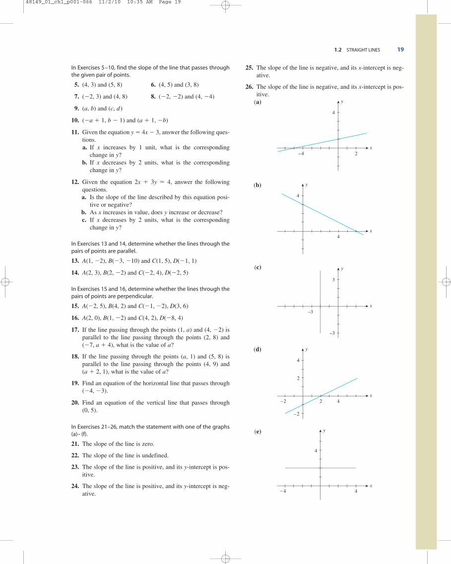
In Exercises 21–26, match the statement with one of the graphs(a)– (f).
21. The slope of the line is zero.
22. The slope of the line is undefined.
23. The slope of the line is positive, and its y-intercept is pos-itive.
24. The slope of the line is positive, and its y-intercept is neg-ative.
25. The slope of the line is negative, and its x-intercept is neg-ative.
26. The slope of the line is negative, and its x-intercept is pos-itive.
(a)
(b)
(c)
(d)
(e)
x
y
4�4
4
x
y
4
4
2
2– 2
– 2
x
y
–3
–3
3
x
y
4
4
x
y
4
–4 2
48149_01_ch1_p001-066 11/2/10 10:35 AM Page 19
20 CHAPTER 1 STRAIGHT LINES AND LINEAR FUNCTIONS
(f)
In Exercises 27–30, find an equation of the line that passesthrough the point and has the indicated slope m.
27. (3, �4); m � 2 28. (2, 4); m � �1
29. (�3, 2); m � 0 30.
In Exercises 31–34, find an equation of the line that passesthrough the given points.
31. (2, 4) and (3, 7) 32. (2, 1) and (2, 5)
33. (1, 2) and (�3, �2) 34. (�1, �2) and (3, �4)
In Exercises 35–38, find an equation of the line that has slope mand y-intercept b.
35. m � 3; b � 4 36. m � �2; b � �1
37. m � 0; b � 5 38.
In Exercises 39–44, write the equation in the slope-interceptform and then find the slope and y-intercept of the correspond-ing line.
39. x � 2y � 0 40. y � 2 � 0
41. 2x � 3y � 9 � 0 42. 3x � 4y � 8 � 0
43. 2x � 4y � 14 44. 5x � 8y � 24 � 0
45. Find an equation of the line that passes through the point(�2, 2) and is parallel to the line 2x � 4y � 8 � 0.
46. Find an equation of the line that passes through the point(�1, 3) and is parallel to the line passing through the points(�2, �3) and (2, 5).
47. Find an equation of the line that passes through the point (2, 4) and is perpendicular to the line 3x � 4y � 22 � 0.
48. Find an equation of the line that passes through the point(1, �2) and is perpendicular to the line passing through thepoints (�2, �1) and (4, 3).
In Exercises 49–54, find an equation of the line that satisfies thegiven condition.
49. The line parallel to the x-axis and 6 units below it
50. The line passing through the origin and parallel to the linepassing through the points (2, 4) and (4, 7)
m � �1
2 ; b �
3
4
11, 2 2 ; m � �1
2
x
y
3
3–3
–2
51. The line passing through the point (a, b) with slope equalto zero
52. The line passing through (�3, 4) and parallel to the x-axis
53. The line passing through (�5, �4) and parallel to the linepassing through (�3, 2) and (6, 8)
54. The line passing through (a, b) with undefined slope
55. Given that the point P(�3, 5) lies on the line kx � 3y �9 � 0, find k.
56. Given that the point P(2, �3) lies on the line �2x � ky �10 � 0, find k.
In Exercises 57–62, sketch the straight line defined by the linearequation by finding the x- and y-intercepts.
Hint: See Example 12.
57. 3x � 2y � 6 � 0 58. 2x � 5y � 10 � 0
59. x � 2y � 4 � 0 60. 2x � 3y � 15 � 0
61. y � 5 � 0 62. �2x � 8y � 24 � 0
63. Show that an equation of a line through the points (a, 0)and (0, b) with a � 0 and b � 0 can be written in the form
(Recall that the numbers a and b are the x- and y-intercepts,respectively, of the line. This form of an equation of a lineis called the intercept form.)
In Exercises 64–67, use the results of Exercise 63 to find an equa-tion of a line with the x- and y-intercepts.
64. x-intercept 3; y-intercept 4
65. x-intercept �2; y-intercept �4
66.
67.
In Exercises 68 and 69, determine whether the points lie on astraight line.
68. A(�1, 7), B(2, �2), and C(5, �9)
69. A(�2, 1), B(1, 7), and C(4, 13)
70. TEMPERATURE CONVERSION The relationship between thetemperature in degrees Fahrenheit (°F) and the temperaturein degrees Celsius (°C) is
a. Sketch the line with the given equation.b. What is the slope of the line? What does it represent?c. What is the F-intercept of the line? What does it repre-
sent?
F �9
5 C � 32
x-intercept 4; y-intercept �1
2
x-intercept �1
2 ; y-intercept
3
4
x
a�
y
b� 1
48149_01_ch1_p001-066 11/2/10 10:35 AM Page 20

71. NUCLEAR PLANT UTILIZATION The United States is not build-ing many nuclear plants, but the ones it has are running atnearly full capacity. The output (as a percentage of totalcapacity) of nuclear plants is described by the equation
y � 1.9467t � 70.082
where t is measured in years, with t � 0 corresponding tothe beginning of 1990.a. Sketch the line with the given equation.b. What are the slope and the y-intercept of the line found
in part (a)?c. Give an interpretation of the slope and the y-intercept of
the line found in part (a).d. If the utilization of nuclear power continued to grow at
the same rate and the total capacity of nuclear plants in theUnited States remained constant, by what year were theplants generating at maximum capacity?
Source: Nuclear Energy Institute.
72. SOCIAL SECURITY CONTRIBUTIONS For wages less than themaximum taxable wage base, Social Security contributions(including those for Medicare) by employees are 7.65% ofthe employee’s wages.a. Find an equation that expresses the relationship between
the wages earned (x) and the Social Security taxes paid( y) by an employee who earns less than the maximumtaxable wage base.
b. For each additional dollar that an employee earns, byhow much is his or her Social Security contributionincreased? (Assume that the employee’s wages are lessthan the maximum taxable wage base.)
c. What Social Security contributions will an employeewho earns $65,000 (which is less than the maximumtaxable wage base) be required to make?
Source: Social Security Administration.
73. COLLEGE ADMISSIONS Using data compiled by the Admis-sions Office at Faber University, college admissions offi-cers estimate that 55% of the students who are offeredadmission to the freshman class at the university will actu-ally enroll.a. Find an equation that expresses the relationship between
the number of students who actually enroll (y) and thenumber of students who are offered admission to theuniversity (x).
b. If the desired freshman class size for the upcoming aca-demic year is 1100 students, how many students shouldbe admitted?
74. WEIGHT OF WHALES The equation W � 3.51L � 192,expressing the relationship between the length L (in feet)and the expected weight W (in British tons) of adult bluewhales, was adopted in the late 1960s by the InternationalWhaling Commission.a. What is the expected weight of an 80-ft blue whale?b. Sketch the straight line that represents the equation.
75. THE NARROWING GENDER GAP Since the founding of theEqual Employment Opportunity Commission and the pas-
1.2 STRAIGHT LINES 21
sage of equal-pay laws, the gulf between men’s andwomen’s earnings has continued to close gradually. At thebeginning of 1990 (t � 0), women’s wages were 68% ofmen’s wages, and by the beginning of 2000 (t � 10),women’s wages were 80% of men’s wages. If this gapbetween women’s and men’s wages continued to narrowlinearly, then women’s wages were what percentage ofmen’s wages at the beginning of 2004?Source: Journal of Economic Perspectives.
76. SALES OF NAVIGATION SYSTEMS The projected number ofnavigation systems (in millions) installed in vehicles inNorth America, Europe, and Japan from 2002 through2006 are shown in the following table (x � 0 correspondsto 2002):
Year, x 0 1 2 3 4
Systems Installed, y 3.9 4.7 5.8 6.8 7.8
a. Plot the annual sales (y) versus the year (x).b. Draw a straight line L through the points corresponding
to 2002 and 2006.c. Derive an equation of the line L.d. Use the equation found in part (c) to estimate the num-
ber of navigation systems installed in 2005. Comparethis figure with the sales for that year.
Source: ABI Research.
77. SALES OF GPS EQUIPMENT The annual sales (in billions ofdollars) of global positioning systems (GPS) equipmentfrom 2000 through 2006 are shown in the following table(x � 0 corresponds to 2000):
Year, x 0 1 2 3 4 5 6
Annual Sales, y 7.9 9.6 11.5 13.3 15.2 17 18.8
a. Plot the annual sales (y) versus the year (x).b. Draw a straight line L through the points corresponding
to 2000 and 2006.c. Derive an equation of the line L.d. Use the equation found in part (c) to estimate the annual
sales of GPS equipment in 2005. Compare this figurewith the projected sales for that year.
Source: ABI Research.
78. IDEAL HEIGHTS AND WEIGHTS FOR WOMEN The Venus HealthClub for Women provides its members with the followingtable, which gives the average desirable weight (in pounds)for women of a given height (in inches):
Height, x 60 63 66 69 72
Weight, y 108 118 129 140 152
a. Plot the weight (y) versus the height (x).b. Draw a straight line L through the points corresponding
to heights of 5 ft and 6 ft.c. Derive an equation of the line L.d. Using the equation of part (c), estimate the average
desirable weight for a woman who is 5 ft, 5 in. tall.
48149_01_ch1_p001-066 11/2/10 10:35 AM Page 21

22 CHAPTER 1 STRAIGHT LINES AND LINEAR FUNCTIONS
79. COST OF A COMMODITY A manufacturer obtained the follow-ing data relating the cost y (in dollars) to the number ofunits (x) of a commodity produced:
UnitsProduced, x 0 20 40 60 80 100
Cost inDollars, y 200 208 222 230 242 250
a. Plot the cost (y) versus the quantity produced (x).b. Draw a straight line through the points (0, 200) and
(100, 250).c. Derive an equation of the straight line of part (b).d. Taking this equation to be an approximation of the
relationship between the cost and the level of produc-tion, estimate the cost of producing 54 units of thecommodity.
80. DIGITAL TV SERVICES The percentage of homes with digitalTV services stood at 5% at the beginning of 1999 (t � 0)and was projected to grow linearly so that, at the beginningof 2003 (t � 4), the percentage of such homes was 25%.a. Derive an equation of the line passing through the
points A(0, 5) and B(4, 25).b. Plot the line with the equation found in part (a).c. Using the equation found in part (a), find the percentage
of homes with digital TV services at the beginning of 2001.
Source: Paul Kagan Associates.
81. SALES GROWTH Metro Department Store’s annual sales (inmillions of dollars) during the past 5 years were
Annual Sales, y 5.8 6.2 7.2 8.4 9.0
Year, x 1 2 3 4 5
a. Plot the annual sales (y) versus the year (x).b. Draw a straight line L through the points corresponding
to the first and fifth years.c. Derive an equation of the line L.d. Using the equation found in part (c), estimate Metro’s
annual sales 4 years from now (x � 9).
82. Is there a difference between the statements “The slope ofa straight line is zero” and “The slope of a straight line doesnot exist (is not defined)”? Explain your answer.
83. Consider the slope-intercept form of a straight line y �mx � b. Describe the family of straight lines obtained bykeepinga. the value of m fixed and allowing the value of b to
vary.b. the value of b fixed and allowing the value of m to
vary.
In Exercises 84–90, determine whether the statement is true orfalse. If it is true, explain why it is true. If it is false, give an exam-ple to show why it is false.
84. Suppose the slope of a line L is and P is a given pointon L. If Q is the point on L lying 4 units to the left of P,then Q is situated 2 units above P.
85. The point (�1, 1) lies on the line with equation 3x �7y � 5.
86. The point (1, k) lies on the line with equation 3x � 4y �12 if and only if .
87. The line with equation Ax � By � C � 0 (B � 0) and theline with equation ax � by � c � 0 (b � 0) are parallel if Ab � aB � 0.
88. If the slope of the line L1 is positive, then the slope of a lineL2 perpendicular to L1 may be positive or negative.
89. The lines with equations ax � by � c1 � 0 and bx � ay �c2 � 0, where a � 0 and b � 0, are perpendicular to eachother.
90. If L is the line with equation Ax � By � C � 0, where A � 0, then L crosses the x-axis at the point (�C>A, 0).
91. Show that two distinct lines with equations a1x � b1y �c1 � 0 and a2 x � b2 y � c2 � 0, respectively, are parallelif and only if a1b2 � b1a2 � 0.Hint: Write each equation in the slope-intercept form and com-pare.
92. Prove that if a line L1 with slope m1 is perpendicular to aline L2 with slope m2, then m1m2 � �1.Hint: Refer to the accompanying figure. Show that m1 � b and m2 � c. Next, apply the Pythagorean Theorem and the distanceformula to the triangles OAC, OCB, and OBA to show that 1 ��bc.
x
y
A(1, b)L1
B(1, c)
L2
C(1, 0)
O
k � 94
�12
48149_01_ch1_p001-066 11/2/10 10:35 AM Page 22

1.2 STRAIGHT LINES 23
1.2 Solutions to Self-Check Exercises
1. The slope of the line that passes through the points (a, 2)and (3, 6) is
Since this line is parallel to a line with slope 4, m must beequal to 4; that is,
or, upon multiplying both sides of the equation by 3 � a,
2. Since the required line L is perpendicular to a line withslope , the slope of L is
Next, using the point-slope form of the equation of a line,we have
3. Substituting x � 3 and y � �3 into the left-hand side of thegiven equation, we find
2(3) � 3(�3) � 12 � 3
which is not equal to zero (the right-hand side). There-fore, (3, �3) does not lie on the line with equation 2x � 3y � 12 � 0. (See the accompanying figure.)
Setting x � 0, we find y � �4, the y-intercept. Next,setting y � 0 gives x � 6, the x-intercept. We now draw theline passing through the points (0, �4) and (6, 0), asshown.
y � 2x � 7
y � 1 � 2x � 6
y � 1�1 2 � 21x � 3 2
m � �1
�12
� 2
�12
a � 2
4a � 8
4 � 12 � 4a
4 � 413 � a 2
4
3 � a� 4
m �6 � 2
3 � a�
4
3 � a
4. a. and b. See the following figure.
c. The slope of L is
Using the point-slope form of the equation of a line withthe point (0, 22.5), we find
y � 22.5 � 2.05(t � 0)
y � 2.05t � 22.5
d. Here the year 2010 corresponds to t � 6, so the esti-mated number of satellite TV subscribers in the UnitedStates in 2010 is
y � 2.05(6) � 22.5 � 34.8
or 34.8 million.
m �30.7 � 22.5
4 � 0� 2.05
1 2 3 4t
Years
y31
22Sate
llite
TV
sub
scri
bers
(in
mill
ions
)
2324252627282930
x
y
– 4
2
– 3
L
(3, – 3)
6
2x � 3y � 12 � 0
Graphing a Straight Line
Graphing UtilityThe first step in plotting a straight line with a graphing utility is to select a suitableviewing window. We usually do this by experimenting. For example, you might firstplot the straight line using the standard viewing window [�10, 10] � [�10, 10]. Ifnecessary, you then might adjust the viewing window by enlarging it or reducing it toobtain a sufficiently complete view of the line or at least the portion of the line that isof interest.
USINGTECHNOLOGY
(continued)
48149_01_ch1_p001-066 11/2/10 10:35 AM Page 23

24 CHAPTER 1 STRAIGHT LINES AND LINEAR FUNCTIONS
EXAMPLE 1 Plot the straight line 2x � 3y � 6 � 0 in the standard viewing window.
Solution The straight line in the standard viewing window is shown in Figure T1.
EXAMPLE 2 Plot the straight line 2x � 3y � 30 � 0 in (a) the standard viewingwindow and (b) the viewing window [�5, 20] � [�5, 20].
Solution
a. The straight line in the standard viewing window is shown in Figure T2a.b. The straight line in the viewing window [�5, 20] � [�5, 20] is shown in Fig-
ure T2b. This figure certainly gives a more complete view of the straight line.
(a) The graph of 2x � 3y � 30 � 0 in (b) The graph of 2x � 3y � 30 � 0 in the standard viewing window the viewing window [�5, 20] � [�5, 20]
ExcelIn the examples and exercises that follow, we assume that you are familiar with thebasic features of Microsoft Excel. Please consult your Excel manual or use Excel’sHelp features to answer questions regarding the standard commands and operatinginstructions for Excel. Here we use Microsoft Excel 2010.*
EXAMPLE 3 Plot the graph of the straight line 2x � 3y � 6 � 0 over the interval[�10, 10].
Solution
1. Write the equation in the slope-intercept form:
2. Create a table of values. First, enter the input values: Enter the values of the end-points of the interval over which you are graphing the straight line. (Recall that weneed only two distinct data points to draw the graph of a straight line. In general,we select the endpoints of the interval over which the straight line is to be drawnas our data points.) In this case, we enter —10 in cell B1 and 10 in cell C1.
Second, enter the formula for computing the y-values: Here, we enter
= —(2/3)*B1+2
in cell B2 and then press .Enter
y � �2
3 x � 2
20
_5
_5 20
10
_10
10_10
10
_10
10_10
FIGURE T1The straight line 2x � 3y � 6 � 0 in thestandard viewing window
FIGURE T2
*Instructions for solving these examples and exercises using Microsoft Excel 2007 are given on CourseMate.
48149_01_ch1_p001-066 11/2/10 10:35 AM Page 24

1.2 STRAIGHT LINES 25
Third, evaluate the function at the other input value: To extend the formula to cellC2, move the pointer to the small black box at the lower right corner of cell B2 (thecell containing the formula). Observe that the pointer now appears as a black � (plussign). Drag this pointer through cell C2 and then release it. The y-value, – 4.66667,corresponding to the x-value in cell C1(10) will appear in cell C2 (Figure T3).
3. Graph the straight line determined by these points. First, highlight the numericalvalues in the table. Here we highlight cells B1:B2 and C1:C2.
Step 1 Click on the ribbon tab and then select from the Chartsgroup. Select the chart subtype in the first row and second column. Achart will then appear on your worksheet.
Step 2 From the Chart Tools group that now appears at the end of the ribbon,click the tab and then select from the Labels
group followed by . Type y =-(2/3)x + 2 and press
. Click from the Labels group and select
followed by . Type x
and then press . Next, click again and select
followed by . Type y and
press .
Step 3 Click which appears on the right side of the graph and
press .
The graph shown in Figure T4 will appear.
If the interval over which the straight line is to be plotted is not specified, then youmight have to experiment to find an appropriate interval for the x-values in your graph.For example, you might first plot the straight line over the interval [�10, 10]. If nec-essary you then might adjust the interval by enlarging it or reducing it to obtain a suf-ficiently complete view of the line or at least the portion of the line that is of interest.
y = -(2/3)x + 210 8 6 4 2 0
�2�4�6
x
y
�5�10�15 0 5 10 15
Delete
Series1
Enter
Vertical TitlePrimary Vertical Axis Title
Axis TitlesEnter
Title Below AxisPrimary Horizontal Axis Title
Axis TitlesEnter
Above Chart
Chart TitleLayout
ScatterInsert
x -10
y 8.6666672
1
-4.66667
10
A B C
FIGURE T3Table of values for x and y
FIGURE T4The graph of over the interval 3�10, 10 4
y � �23 x � 2
(continued)
Note: Boldfaced words/characters enclosed in a box (for example, ) indicate that an action (click, select, or press) isrequired. Words/characters printed blue (for example, Chart Type) indicate words/characters that appear on the screen.Words/characters printed in a monospace font (for example, =(—2/3)*A2+2) indicate words/characters that need to be typedand entered.
Enter
48149_01_ch1_p001-066 11/2/10 10:35 AM Page 25
26 CHAPTER 1 STRAIGHT LINES AND LINEAR FUNCTIONS
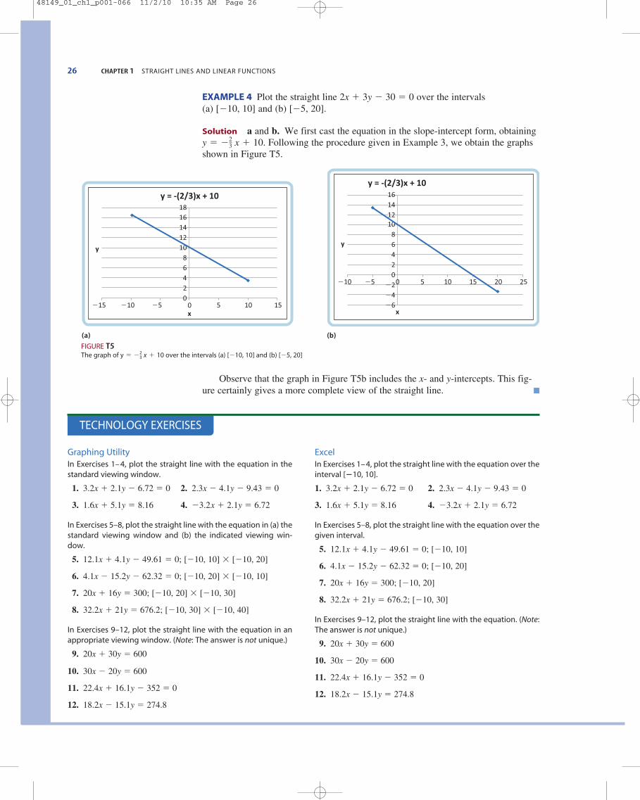
EXAMPLE 4 Plot the straight line 2x � 3y � 30 � 0 over the intervals (a) [�10, 10] and (b) [�5, 20].
Solution a and b. We first cast the equation in the slope-intercept form, obtaining. Following the procedure given in Example 3, we obtain the graphs
shown in Figure T5.y � �2
3 x � 10
(a) (b)
FIGURE T5The graph of over the intervals (a) [�10, 10] and (b) [�5, 20]y � �2
3 x � 10
Graphing UtilityIn Exercises 1–4, plot the straight line with the equation in thestandard viewing window.
1. 3.2x � 2.1y � 6.72 � 0 2. 2.3x � 4.1y � 9.43 � 0
3. 1.6x � 5.1y � 8.16 4. �3.2x � 2.1y � 6.72
In Exercises 5–8, plot the straight line with the equation in (a) thestandard viewing window and (b) the indicated viewing win-dow.
5. 12.1x � 4.1y � 49.61 � 0; [�10, 10] � [�10, 20]
6. 4.1x � 15.2y � 62.32 � 0; [�10, 20] � [�10, 10]
7. 20x � 16y � 300; [�10, 20] � [�10, 30]
8. 32.2x � 21y � 676.2; [�10, 30] � [�10, 40]
In Exercises 9–12, plot the straight line with the equation in anappropriate viewing window. (Note: The answer is not unique.)
9. 20x � 30y � 600
10. 30x � 20y � 600
11. 22.4x � 16.1y � 352 � 0
12. 18.2x � 15.1y � 274.8
ExcelIn Exercises 1–4, plot the straight line with the equation over theinterval [�10, 10].
1. 3.2x � 2.1y � 6.72 � 0 2. 2.3x � 4.1y � 9.43 � 0
3. 1.6x � 5.1y � 8.16 4. �3.2x � 2.1y � 6.72
In Exercises 5–8, plot the straight line with the equation over thegiven interval.
5. 12.1x � 4.1y � 49.61 � 0; [�10, 10]
6. 4.1x � 15.2y � 62.32 � 0; [�10, 20]
7. 20x � 16y � 300; [�10, 20]
8. 32.2x � 21y � 676.2; [�10, 30]
In Exercises 9–12, plot the straight line with the equation. (Note:The answer is not unique.)
9. 20x � 30y � 600
10. 30x � 20y � 600
11. 22.4x � 16.1y � 352 � 0
12. 18.2x � 15.1y � 274.8
TECHNOLOGY EXERCISES
y = -(2/3)x + 10
1618
14 1210
86420
x
y
�5�10�15 0 5 10 15
y = -(2/3)x + 10
10 8 6 4
161412
2 0
�2�4�6
x
y
�5�10 0 5 1510 20 25
Observe that the graph in Figure T5b includes the x- and y-intercepts. This fig-ure certainly gives a more complete view of the straight line.
48149_01_ch1_p001-066 11/2/10 10:35 AM Page 26

1.3 LINEAR FUNCTIONS AND MATHEMATICAL MODELS 27
FIGURE 28
Mathematical Models
Regardless of the field from which a real-world problem is drawn, the problem issolved by analyzing it through a process called mathematical modeling. The foursteps in this process, as illustrated in Figure 28, follow.
Mathematical Modeling
1. Formulate Given a real-world problem, our first task is to formulate the problemusing the language of mathematics. The many techniques that are used in construct-ing mathematical models range from theoretical consideration of the problem on theone extreme to an interpretation of data associated with the problem on the other. Forexample, the mathematical model giving the accumulated amount at any time whena certain sum of money is deposited in the bank can be derived theoretically (seeChapter 5). On the other hand, many of the mathematical models in this book are con-structed by studying the data associated with the problem. In Section 1.5, we see howlinear equations (models) can be constructed from a given set of data points. Also, inthe ensuing chapters we will see how other mathematical models, including statisti-cal and probability models, are used to describe and analyze real-world situations.
2. Solve Once a mathematical model has been constructed, we can use the appropri-ate mathematical techniques, which we will develop throughout the book, to solvethe problem.
3. Interpret Bearing in mind that the solution obtained in Step 2 is just the solutionof the mathematical model, we need to interpret these results in the context of theoriginal real-world problem.
4. Test Some mathematical models of real-world applications describe the situationswith complete accuracy. For example, the model describing a deposit in a bankaccount gives the exact accumulated amount in the account at any time. But othermathematical models give, at best, an approximate description of the real-world prob-lem. In this case, we need to test the accuracy of the model by observing how well itdescribes the original real-world problem and how well it predicts past and/or futurebehavior. If the results are unsatisfactory, then we may have to reconsider the assump-tions made in the construction of the model or, in the worst case, return to Step 1.
We now look at an important way of describing the relationship between twoquantities using the notion of a function. As you will see subsequently, many mathe-matical models are represented by functions.
Functions
A manufacturer would like to know how his company’s profit is related to its produc-tion level; a biologist would like to know how the population of a certain culture ofbacteria will change with time; a psychologist would like to know the relationshipbetween the learning time of an individual and the length of a vocabulary list; and achemist would like to know how the initial speed of a chemical reaction is related tothe amount of substrate used. In each instance, we are concerned with the same ques-
Interpret
FormulateReal-worldproblem
Test Solve
Mathematicalmodel
Solution ofmathematical model
Solution ofreal-world problem
1.3 Linear Functions and Mathematical Models
48149_01_ch1_p001-066 11/2/10 10:35 AM Page 27

28 CHAPTER 1 STRAIGHT LINES AND LINEAR FUNCTIONS
tion: How does one quantity depend on another? The relationship between two quan-tities is conveniently described in mathematics by using the concept of a function.
The number y is normally denoted by f (x), read “f of x,” emphasizing the dependency of y on x.
An example of a function may be drawn from the familiar relationship betweenthe area of a circle and its radius. Let x and y denote the radius and area of a circle,respectively. From elementary geometry, we have
This equation defines y as a function of x, since for each admissible value of x (a positive number representing the radius of a certain circle), there corresponds pre-cisely one number y � px2 giving the area of the circle. This area function may bewritten as
(7)
For example, to compute the area of a circle with a radius of 5 inches, we simplyreplace x in Equation (7) by the number 5. Thus, the area of the circle is
or 25p square inches.Suppose we are given the function y � f(x).* The variable x is referred to as the
independent variable, and the variable y is called the dependent variable. The set ofall values that may be assumed by x is called the domain of the function f, and the setcomprising all the values assumed by y � f(x) as x takes on all possible values in itsdomain is called the range of the function f. For the area function (7), the domain of f isthe set of all positive numbers x, and the range of f is the set of all positive numbers y.
We now focus our attention on an important class of functions known as linearfunctions. Recall that a linear equation in x and y has the form Ax � By � C � 0,where A, B, and C are constants and A and B are not both zero. If B � 0, the equationcan always be solved for y in terms of x; in fact, as we saw in Section 1.2, the equa-tion may be cast in the slope-intercept form:
y � mx � b (m, b constants) (8)
Equation (8) defines y as a function of x. The domain and range of this functionare the set of all real numbers. Furthermore, the graph of this function, as we saw inSection 1.2, is a straight line in the plane. For this reason, the function f (x) � mx � b iscalled a linear function.
Linear functions play an important role in the quantitative analysis of business and economic problems. First, many problems that arise in these and other fields are
Linear Function
The function f defined by
f 1x 2 � mx � b
where m and b are constants, is called a linear function.
f 15 2 � p52 � 25p
f 1x 2 � px 2
y � px 2
Function
A function f is a rule that assigns to each value of x one and only one value of y.
*It is customary to refer to a function f as f (x).
48149_01_ch1_p001-066 11/2/10 10:35 AM Page 28
linear in nature or are linear in the intervals of interest and thus can be formulated interms of linear functions. Second, because linear functions are relatively easy to workwith, assumptions involving linearity are often made in the formulation of problems.In many cases, these assumptions are justified, and acceptable mathematical modelsare obtained that approximate real-life situations.
The following example uses a linear function to model the market for U.S. health-care costs. In Section 1.5, we show how this model is constructed using the least-squares technique. (In “Using Technology” on pages 60–63, you will be asked to usea graphing calculator or Excel to construct other mathematical models from raw data.)
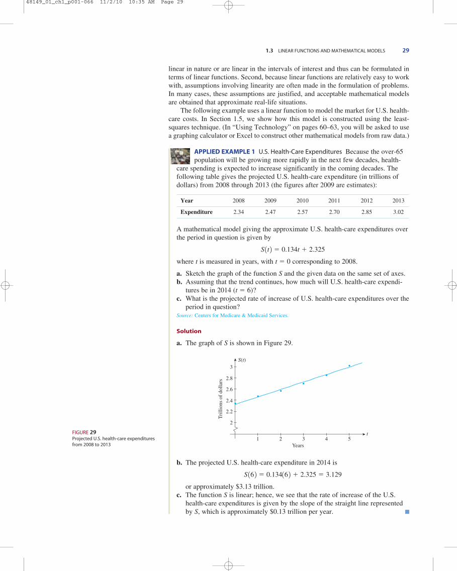
APPLIED EXAMPLE 1 U.S. Health-Care Expenditures Because the over-65population will be growing more rapidly in the next few decades, health-
care spending is expected to increase significantly in the coming decades. Thefollowing table gives the projected U.S. health-care expenditure (in trillions ofdollars) from 2008 through 2013 (the figures after 2009 are estimates):
Year 2008 2009 2010 2011 2012 2013
Expenditure 2.34 2.47 2.57 2.70 2.85 3.02
A mathematical model giving the approximate U.S. health-care expenditures overthe period in question is given by
S 1t 2 � 0.134t � 2.325
where t is measured in years, with t � 0 corresponding to 2008.
a. Sketch the graph of the function S and the given data on the same set of axes.b. Assuming that the trend continues, how much will U.S. health-care expendi-
tures be in 2014 (t � 6)?c. What is the projected rate of increase of U.S. health-care expenditures over the
period in question?Source: Centers for Medicare & Medicaid Services.
Solution
a. The graph of S is shown in Figure 29.
b. The projected U.S. health-care expenditure in 2014 is
S 16 2 � 0.13416 2 � 2.325 � 3.129
or approximately $3.13 trillion.c. The function S is linear; hence, we see that the rate of increase of the U.S.
health-care expenditures is given by the slope of the straight line representedby S, which is approximately $0.13 trillion per year.
1.3 LINEAR FUNCTIONS AND MATHEMATICAL MODELS 29
FIGURE 29Projected U.S. health-care expendituresfrom 2008 to 2013
t1 2 3 4 5
S(t)
2
2.2
2.4
2.6
2.8
3
Years
Tri
llion
s of
dol
lars
48149_01_ch1_p001-066 11/2/10 10:35 AM Page 29

In the rest of this section, we look at several applications that can be modeled byusing linear functions.
Simple Depreciation
We first discussed linear depreciation in Section 1.2 as a real-world application ofstraight lines. The following example illustrates how to derive an equation describingthe book value of an asset that is being depreciated linearly.
APPLIED EXAMPLE 2 Linear Depreciation A network server has an origi-nal value of $10,000 and is to be depreciated linearly over 5 years
with a $3000 scrap value. Find an expression giving the book value at the end ofyear t. What will be the book value of the server at the end of the second year?What is the rate of depreciation of the server?
Solution Let V(t) denote the network server’s book value at the end of the t thyear. Since the depreciation is linear, V is a linear function of t. Equivalently, thegraph of the function is a straight line. Now, to find an equation of the straightline, observe that V � 10,000 when t � 0; this tells us that the line passes throughthe point (0, 10,000). Similarly, the condition that V � 3000 when t � 5 says thatthe line also passes through the point (5, 3000). The slope of the line is given by
Using the point-slope form of the equation of a line with the point (0, 10,000)and the slope m � �1400, we have
the required expression. The book value at the end of the second year is given by
V 12 2 � �1400 12 2 � 10,000 � 7200
or $7200. The rate of depreciation of the server is given by the negative of the slope ofthe depreciation line. Since the slope of the line is m � �1400, the rate of depreciationis $1400 per year. The graph of V � �1400t � 10,000 is sketched in Figure 30.
Linear Cost, Revenue, and Profit Functions
Whether a business is a sole proprietorship or a large corporation, the owner or chiefexecutive must constantly keep track of operating costs, revenue resulting from thesale of products or services, and, perhaps most important, the profits realized. Threefunctions provide management with a measure of these quantities: the total cost func-tion, the revenue function, and the profit function.
Cost, Revenue, and Profit Functions
Let x denote the number of units of a product manufactured or sold. Then, thetotal cost function is
C 1x 2 � Total cost of manufacturing x units of the product
The revenue function is
R 1x 2 � Total revenue realized from the sale of x units of the product
The profit function is
P 1x 2 � Total profit realized from manufacturing and selling x units of the product
V � �1400t � 10,000
V � 10,000 � �14001t � 0 2
m �10,000 � 3000
0 � 5� �
7000
5� �1400
30 CHAPTER 1 STRAIGHT LINES AND LINEAR FUNCTIONS
t1 2 3 4 5
V ($)
10,000
3000
Years
(5, 3000)
FIGURE 30Linear depreciation of an asset
48149_01_ch1_p001-066 11/2/10 10:35 AM Page 30

Generally speaking, the total cost, revenue, and profit functions associated with acompany will probably be nonlinear (these functions are best studied using the toolsof calculus). But linear cost, revenue, and profit functions do arise in practice, and wewill consider such functions in this section. Before deriving explicit forms of thesefunctions, we need to recall some common terminology.
The costs that are incurred in operating a business are usually classified into twocategories. Costs that remain more or less constant regardless of the firm’s activitylevel are called fixed costs. Examples of fixed costs are rental fees and executivesalaries. Costs that vary with production or sales are called variable costs. Examplesof variable costs are wages and costs for raw materials.
Suppose a firm has a fixed cost of F dollars, a production cost of c dollars per unit,and a selling price of s dollars per unit. Then the cost function C(x), the revenue func-tion R(x), and the profit function P(x) for the firm are given by
Revenue � cost
where x denotes the number of units of the commodity produced and sold. The func-tions C, R, and P are linear functions of x.
APPLIED EXAMPLE 3 Profit Functions Puritron, a manufacturer of waterfilters, has a monthly fixed cost of $20,000, a production cost of $20 per
unit, and a selling price of $30 per unit. Find the cost function, the revenue func-tion, and the profit function for Puritron.
Solution Let x denote the number of units produced and sold. Then
Linear Demand and Supply Curves
In a free-market economy, consumer demand for a particular commodity depends onthe commodity’s unit price. A demand equation expresses this relationship betweenthe unit price and the quantity demanded. The corresponding graph of the demandequation is called a demand curve. In general, the quantity demanded of a commod-ity decreases as its unit price increases, and vice versa. Accordingly, a demand function defined by p � f (x), where p measures the unit price and x measures thenumber of units of the commodity, is generally characterized as a decreasing functionof x ; that is, p � f (x) decreases as x increases.
The simplest demand function is defined by a linear equation in x and p, whereboth x and p assume only positive values. Its graph is a straight line having a negativeslope. Thus, the demand curve in this case is that part of the graph of a straight linethat lies in the first quadrant (Figure 31).
APPLIED EXAMPLE 4 Demand Functions The quantity demanded of theSentinel iPod™ alarm clock is 48,000 units when the unit price is $8. At
$12 per unit, the quantity demanded drops to 32,000 units. Find the demandequation, assuming that it is linear. What is the unit price corresponding to a
� 10x � 20,000
� 30x � 120x � 20,000 2P1x 2 � R1x 2 � C1x 2R1x 2 � 30x
C1x 2 � 20x � 20,000
� 1s � c 2x � F
P1x 2 � R1x 2 � C1x 2R1x 2 � sx
C1x 2 � cx � F
1.3 LINEAR FUNCTIONS AND MATHEMATICAL MODELS 31
p
x
FIGURE 31A graph of a linear demand function
48149_01_ch1_p001-066 11/2/10 10:35 AM Page 31
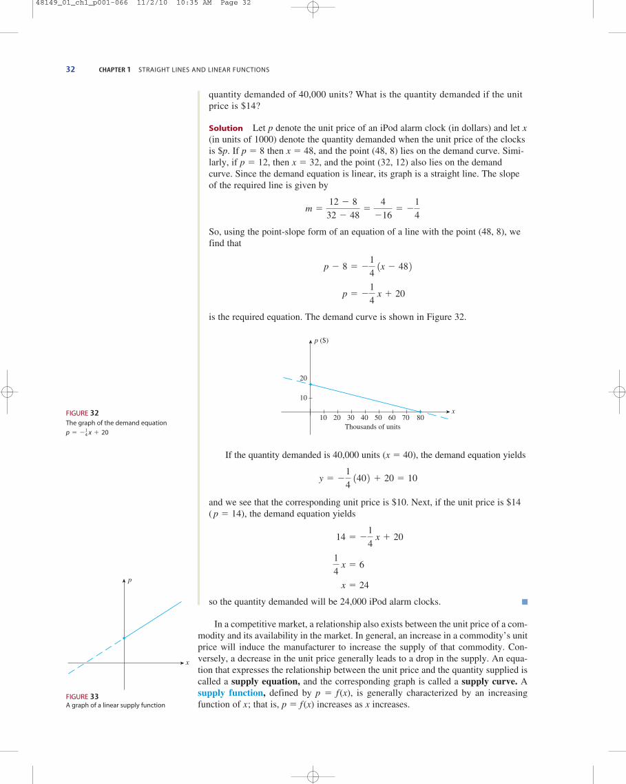
quantity demanded of 40,000 units? What is the quantity demanded if the unitprice is $14?
Solution Let p denote the unit price of an iPod alarm clock (in dollars) and let x(in units of 1000) denote the quantity demanded when the unit price of the clocksis $p. If p � 8 then x � 48, and the point (48, 8) lies on the demand curve. Simi-larly, if p � 12, then x � 32, and the point (32, 12) also lies on the demandcurve. Since the demand equation is linear, its graph is a straight line. The slopeof the required line is given by
So, using the point-slope form of an equation of a line with the point (48, 8), wefind that
is the required equation. The demand curve is shown in Figure 32.
If the quantity demanded is 40,000 units (x � 40), the demand equation yields
and we see that the corresponding unit price is $10. Next, if the unit price is $14 ( p � 14), the demand equation yields
so the quantity demanded will be 24,000 iPod alarm clocks.
In a competitive market, a relationship also exists between the unit price of a com-modity and its availability in the market. In general, an increase in a commodity’s unitprice will induce the manufacturer to increase the supply of that commodity. Con-versely, a decrease in the unit price generally leads to a drop in the supply. An equa-tion that expresses the relationship between the unit price and the quantity supplied iscalled a supply equation, and the corresponding graph is called a supply curve. Asupply function, defined by p � f (x), is generally characterized by an increasingfunction of x; that is, p � f (x) increases as x increases.
x � 24
1
4 x � 6
14 � �1
4 x � 20
y � �1
4 140 2 � 20 � 10
x10 20 30 40 50 60 70 80
p ($)
20
10
Thousands of units
p � �1
4 x � 20
p � 8 � �1
4 1x � 48 2
m �12 � 8
32 � 48�
4
�16� �
1
4
32 CHAPTER 1 STRAIGHT LINES AND LINEAR FUNCTIONS
p
x
FIGURE 33A graph of a linear supply function
FIGURE 32The graph of the demand equation
p � �14 x � 20
48149_01_ch1_p001-066 11/2/10 10:35 AM Page 32

As in the case of a demand equation, the simplest supply equation is a linear equa-tion in p and x, where p and x have the same meaning as before but the line has a pos-itive slope. The supply curve corresponding to a linear supply function is that part ofthe straight line that lies in the first quadrant (Figure 33).
APPLIED EXAMPLE 5 Supply Functions The supply equation for a com-modity is given by 4p � 5x � 120, where p is measured in dollars and x is
measured in units of 100.
a. Sketch the corresponding curve.b. How many units will be marketed when the unit price is $55?
Solution
a. Setting x � 0, we find the p-intercept to be 30. Next, setting p � 0, we findthe x-intercept to be �24. The supply curve is sketched in Figure 34.
b. Substituting p � 55 in the supply equation, we have 4(55) � 5x � 120 or x � 20, so the amount marketed will be 2000 units.
1.3 LINEAR FUNCTIONS AND MATHEMATICAL MODELS 33
1.3 Exercises
1.3 Self-Check Exercises
1.3 Concept Questions
x10 20 30 40 50
p ($)
60
50
40
30
10
Hundreds of units
20
FIGURE 34The graph of the supply equation 4p � 5x � 120
1. A manufacturer has a monthly fixed cost of $60,000 and aproduction cost of $10 for each unit produced. The productsells for $15/unit.a. What is the cost function?b. What is the revenue function?c. What is the profit function?d. Compute the profit (loss) corresponding to production
levels of 10,000 and 14,000 units/month.
2. The quantity demanded for a certain make of 30-in. �52-in. area rug is 500 when the unit price is $100. For each$20 decrease in the unit price, the quantity demandedincreases by 500 units. Find the demand equation andsketch its graph.
Solutions to Self-Check Exercises 1.3 can be found on page 36.
1. a. What is a function? Give an example.b. What is a linear function? Give an example.c. What is the domain of a linear function? The range?d. What is the graph of a linear function?
2. What is the general form of a linear cost function? A linearrevenue function? A linear profit function?
3. Is the slope of a linear demand curve positive or negative?The slope of a linear supply curve?
In Exercises 1–10, determine whether the equation defines y as alinear function of x. If so, write it in the form y � mx � b.
1. 2x � 3y � 6 2. �2x � 4y � 7
3. x � 2y � 4 4. 2x � 3y � 8
5. 2x � 4y � 9 � 0 6. 3x � 6y � 7 � 0
7. 2x2 � 8y � 4 � 0 8. 31x � 4y � 0
9. 2x � 3y2 � 8 � 0 10.
11. A manufacturer has a monthly fixed cost of $40,000 and aproduction cost of $8 for each unit produced. The productsells for $12/unit.a. What is the cost function?b. What is the revenue function?c. What is the profit function?d. Compute the profit (loss) corresponding to production
levels of 8000 and 12,000 units.
2x � 1y � 4 � 0
VIDEO
48149_01_ch1_p001-066 11/2/10 10:35 AM Page 33

34 CHAPTER 1 STRAIGHT LINES AND LINEAR FUNCTIONS
12. A manufacturer has a monthly fixed cost of $100,000 anda production cost of $14 for each unit produced. The prod-uct sells for $20/unit.a. What is the cost function?b. What is the revenue function?c. What is the profit function?d. Compute the profit (loss) corresponding to production
levels of 12,000 and 20,000 units.
13. Find the constants m and b in the linear function f(x) �mx � b such that f (0) � 2 and f (3) � �1.
14. Find the constants m and b in the linear function f(x) �mx � b such that f (2) � 4 and the straight line representedby f has slope �1.
15. LINEAR DEPRECIATION An office building worth $1 millionwhen completed in 2005 is being depreciated linearly over50 years. What was the book value of the building in 2010?What will it be in 2015? (Assume that the scrap value is $0.)
16. LINEAR DEPRECIATION An automobile purchased for use bythe manager of a firm at a price of $24,000 is to be depre-ciated using the straight-line method over 5 years. Whatwill be the book value of the automobile at the end of 3 years? (Assume that the scrap value is $0.)
17. CONSUMPTION FUNCTIONS A certain economy’s consump-tion function is given by the equation
C 1x 2 � 0.75x � 6
where C(x) is the personal consumption expenditure in bil-lions of dollars and x is the disposable personal income inbillions of dollars. Find C(0), C(50), and C(100).
18. SALES TAX In a certain state, the sales tax T on the amountof taxable goods is 6% of the value of the goods purchased(x), where both T and x are measured in dollars.a. Express T as a function of x.b. Find T(200) and T(5.60).
19. SOCIAL SECURITY BENEFITS Social Security recipients receivean automatic cost-of-living adjustment (COLA) once eachyear. Their monthly benefit is increased by the same per-centage that consumer prices have increased during the pre-ceding year. Suppose consumer prices have increased by5.3% during the preceding year.a. Express the adjusted monthly benefit of a Social Secu-
rity recipient as a function of his or her current monthlybenefit.
b. If Carlos Garcia’s monthly Social Security benefit isnow $1020, what will be his adjusted monthly benefit?
20. PROFIT FUNCTIONS AutoTime, a manufacturer of 24-hr vari-able timers, has a monthly fixed cost of $48,000 and a pro-duction cost of $8 for each timer manufactured. The timerssell for $14 each.a. What is the cost function?b. What is the revenue function?c. What is the profit function?d. Compute the profit (loss) corresponding to produc-
tion levels of 4000, 6000, and 10,000 timers, respec-tively.
21. PROFIT FUNCTIONS The management of TMI finds that themonthly fixed costs attributable to the production of their100-watt light bulbs is $12,100.00. If the cost of producingeach twin-pack of light bulbs is $0.60 and each twin-packsells for $1.15, find the company’s cost function, revenuefunction, and profit function.
22. LINEAR DEPRECIATION In 2007, National Textile installed anew machine in one of its factories at a cost of $250,000.The machine is depreciated linearly over 10 years with ascrap value of $10,000.a. Find an expression for the machine’s book value in the
t th year of use (0 � t � 10).b. Sketch the graph of the function of part (a).c. Find the machine’s book value in 2011.d. Find the rate at which the machine is being depreciated.
23. LINEAR DEPRECIATION A workcenter system purchased at acost of $60,000 in 2010 has a scrap value of $12,000 at theend of 4 years. If the straight-line method of depreciationis used,a. Find the rate of depreciation.b. Find the linear equation expressing the system’s book
value at the end of t years.c. Sketch the graph of the function of part (b).d. Find the system’s book value at the end of the third
year.
24. LINEAR DEPRECIATION Suppose an asset has an originalvalue of $C and is depreciated linearly over N years with ascrap value of $S. Show that the asset’s book value at theend of the t th year is described by the function
Hint: Find an equation of the straight line passing through thepoints (0, C) and (N, S). (Why?)
25. Rework Exercise 15 using the formula derived in Exer-cise 24.
26. Rework Exercise 16 using the formula derived in Exer-cise 24.
27. DRUG DOSAGES A method sometimes used by pediatriciansto calculate the dosage of medicine for children is based onthe child’s surface area. If a denotes the adult dosage (inmilligrams) and if S is the child’s surface area (in squaremeters), then the child’s dosage is given by
a. Show that D is a linear function of S.Hint: Think of D as having the form D(S) � mS � b. What are theslope m and the y-intercept b?b. If the adult dose of a drug is 500 mg, how much should
a child whose surface area is 0.4 m2 receive?
28. DRUG DOSAGES Cowling’s Rule is a method for calculatingpediatric drug dosages. If a denotes the adult dosage (inmilligrams) and if t is the child’s age (in years), then the
D1S 2 �Sa
1.7
V1t 2 � C � aC � S
Nb t
48149_01_ch1_p001-066 11/2/10 10:35 AM Page 34

child’s dosage is given by
a. Show that D is a linear function of t.Hint: Think of D(t) as having the form D(t) � mt � b. What isthe slope m and the y-intercept b?
b. If the adult dose of a drug is 500 mg, how much shoulda 4-year-old child receive?
29. BROADBAND INTERNET HOUSEHOLDS The number of U.S.broadband Internet households stood at 20 million at thebeginning of 2002 and was projected to grow at the rate of6.5 million households per year for the next 8 years.a. Find a linear function f (t) giving the projected number
of U.S. broadband Internet households (in millions) inyear t, where t � 0 corresponds to the beginning of2002.
b. What was the projected number of U.S. broadbandInternet households at the beginning of 2010?
Source: Jupiter Research.
30. DIAL-UP INTERNET HOUSEHOLDS The number of U.S. dial-upInternet households stood at 42.5 million at the beginningof 2004 and was projected to decline at the rate of 3.9 million households per year for the next 6 years.a. Find a linear function f giving the projected U.S. dial-up
Internet households (in millions) in year t, where t � 0corresponds to the beginning of 2004.
b. What was the projected number of U.S. dial-up Internethouseholds at the beginning of 2010?
Source: Strategy Analytics, Inc.
31. CELSIUS AND FAHRENHEIT TEMPERATURES The relationshipbetween temperature measured on the Celsius scale and onthe Fahrenheit scale is linear. The freezing point is 0°C and32°F, and the boiling point is 100°C and 212°F.a. Find an equation giving the relationship between the
temperature F measured on the Fahrenheit scale and thetemperature C measured on the Celsius scale.
b. Find F as a function of C and use this formula to deter-mine the temperature in Fahrenheit corresponding to atemperature of 20°C.
c. Find C as a function of F and use this formula to deter-mine the temperature in Celsius corresponding to a tem-perature of 70°F.
32. CRICKET CHIRPING AND TEMPERATURE Entomologists havediscovered that a linear relationship exists between the rateof chirping of crickets of a certain species and the air tem-perature. When the temperature is 70°F, the crickets chirpat the rate of 120 chirps/min, and when the temperature is80°F, they chirp at the rate of 160 chirps/min.a. Find an equation giving the relationship between the air
temperature T and the number of chirps per minute N ofthe crickets.
b. Find N as a function of T, and use this function to deter-mine the rate at which the crickets chirp when the tem-perature is 102°F.
D 1t 2 � a t � 1
24ba
1.3 LINEAR FUNCTIONS AND MATHEMATICAL MODELS 35
For each demand equation in Exercises 33–36, where x repre-sents the quantity demanded in units of 1000 and p is the unitprice in dollars, (a) sketch the demand curve, and (b) determinethe quantity demanded corresponding to the given unit price p.
33. 2x � 3p � 18 � 0; p � 4
34. 5p � 4x � 80 � 0; p � 10
35. p � �3x � 60; p � 30
36. p � �0.4x � 120; p � 80
37. DEMAND FUNCTIONS At a unit price of $55, the quantitydemanded of a certain commodity is 1000 units. At a unitprice of $85, the demand drops to 600 units. Given that itis linear, find the demand equation. Above what price willthere be no demand? What quantity would be demanded ifthe commodity were free?
38. DEMAND FUNCTIONS The quantity demanded for a certainbrand of portable CD players is 200 units when the unitprice is set at $90. The quantity demanded is 1200 unitswhen the unit price is $40. Find the demand equation, andsketch its graph.
39. DEMAND FUNCTIONS Assume that a certain commodity’sdemand equation has the form p � ax � b, where x is thequantity demanded and p is the unit price in dollars. Sup-pose the quantity demanded is 1000 units when the unitprice is $9.00 and 6000 when the unit price is $4.00. Whatis the quantity demanded when the unit price is $7.50?
40. DEMAND FUNCTIONS The demand equation for the Sicardsports watch is
p � �0.025x � 50
where x is the quantity demanded per week and p is the unitprice in dollars. Sketch the graph of the demand equation.What is the highest price (theoretically) anyone would payfor the watch?
For each supply equation in Exercises 41–44, where x is thequantity supplied in units of 1000 and p is the unit price in dol-lars, (a) sketch the supply curve, and (b) determine the numberof units of the commodity the supplier will make available in themarket at the given unit price.
41. 3x � 4p � 24 � 0; p � 8
42.
43. p � 2x � 10; p � 14
44.
45. SUPPLY FUNCTIONS Suppliers of a certain brand of digitalvoice recorders will make 10,000 available in the market ifthe unit price is $45. At a unit price of $50, 20,000 unitswill be made available. Assuming that the relationshipbetween the unit price and the quantity supplied is linear,
p �1
2 x � 20; p � 28
1
2 x �
2
3 p � 12 � 0; p � 24
48149_01_ch1_p001-066 11/2/10 10:35 AM Page 35

36 CHAPTER 1 STRAIGHT LINES AND LINEAR FUNCTIONS
derive the supply equation. Sketch the supply curve, anddetermine the quantity suppliers will make available whenthe unit price is $70.
46. SUPPLY FUNCTIONS Producers will make 2000 refrigeratorsavailable when the unit price is $330. At a unit price of$390, 6000 refrigerators will be marketed. Find the equa-tion relating the unit price of a refrigerator to the quantitysupplied if the equation is known to be linear. How manyrefrigerators will be marketed when the unit price is $450?What is the lowest price at which a refrigerator will bemarketed?
In Exercises 47 and 48, determine whether the statement is trueor false. If it is true, explain why it is true. If it is false, give anexample to show why it is false.
47. Suppose C(x) � cx � F and R(x) � sx are the cost and rev-enue functions of a certain firm. Then the firm is making aprofit if its level of production is less than F/(s � c).
48. If p � mx � b is a linear demand curve, then it is generallytrue that m � 0.
1.3 Solutions to Self-Check Exercises
1. Let x denote the number of units produced and sold. Thena. C 1x 2 � 10x � 60,000b. R 1x 2 � 15xc. P 1x 2 � R 1x 2 � C 1x 2 � 15x � 110x � 60,000 2
� 5x � 60,000d. P 110,000 2 � 5 110,000 2 � 60,000
� �10,000or a loss of $10,000 per month.
P 114,000 2 � 5 114,000 2 � 60,000� 10,000
or a profit of $10,000 per month.
2. Let p denote the price of a rug (in dollars), and let x denotethe quantity of rugs demanded when the unit price is $p.The condition that the quantity demanded is 500 when theunit price is $100 tells us that the demand curve passesthrough the point (500, 100). Next, the condition that foreach $20 decrease in the unit price, the quantity demandedincreases by 500 tells us that the demand curve is linearand that its slope is given by , or . Therefore, let-� 1
25� 20500
To determine b, use the fact that the straight line passesthrough (500, 100) to obtain
or b � 120. Therefore, the required equation is
The graph of the demand curve issketched in the following figure.
x1000 2000 3000
p ($)
120
p � � 125 x � 120
p � �1
25 x � 120
100 � �1
25 1500 2 � b
USINGTECHNOLOGY
Evaluating a Function
Graphing UtilityA graphing utility can be used to find the value of a function f at a given point with min-imal effort. However, to find the value of y for a given value of x in a linear equationsuch as Ax � By � C � 0, the equation must first be cast in the slope-intercept form y � mx � b, thus revealing the desired rule f(x) � mx � b for y as a function of x.
EXAMPLE 1 Consider the equation 2x � 5y � 7.
a. Plot the straight line with the given equation in the standard viewing window.b. Find the value of y when x � 2 and verify your result by direct computation.c. Find the value of y when x � 1.732.
ting in the demand equation
p � mx � b
we find
p � �1
25 x � b
m � � 125
48149_01_ch1_p001-066 11/3/10 11:36 AM Page 36

Solution
a. The straight line with equation 2x � 5y � 7 or, equivalently, in thestandard viewing window is shown in Figure T1.
b. Using the evaluation function of the graphing utility and the value of 2 for x, wefind y � 0.6. This result is verified by computing
when x � 2.c. Once again using the evaluation function of the graphing utility, this time with
the value 1.732 for x, we find y � 0.7072.
When evaluating f (x) at x � a, remember that the number a must lie betweenxMin and xMax.
APPLIED EXAMPLE 2 Market for Cholesterol-Reducing Drugs In a studyconducted in early 2000, experts projected a rise in the market for
cholesterol-reducing drugs. The U.S. market (in billions of dollars) for such drugs from 1999 through 2004 is approximated by
M 1t 2 � 1.95t � 12.19
where t is measured in years, with t � 0 corresponding to 1999.
a. Plot the graph of the function M in the viewing window [0, 5] � [0, 25].b. What was the estimated market for cholesterol-reducing drugs in 2005
(t � 6)?c. What was the rate of increase of the market for cholesterol-reducing drugs
over the period in question?Source: S. G. Cowen.
Solution
a. The graph of M is shown in Figure T2.
b. The market in 2005 for cholesterol-reducing drugs was approximately
M 16 2 � 1.95 16 2 � 12.19 � 23.89
or $23.89 billion.
50
25
y � �2
5 12 2 �
7
5� �
4
5�
7
5�
3
5� 0.6
y � �25 x � 7
5
1.3 LINEAR FUNCTIONS AND MATHEMATICAL MODELS 37
FIGURE T1The straight line 2x � 5y � 7 in the stan-dard viewing window
10
_10
10_10
(continued)
FIGURE T2The graph of M in the viewing window [0, 5] � [0, 25]
48149_01_ch1_p001-066 11/2/10 10:35 AM Page 37

38 CHAPTER 1 STRAIGHT LINES AND LINEAR FUNCTIONS
c. The function M is linear; hence, we see that the rate of increase of the marketfor cholesterol-reducing drugs is given by the slope of the straight line repre-sented by M, which is approximately $1.95 billion per year.
ExcelExcel can be used to find the value of a function at a given value with minimal effort.However, to find the value of y for a given value of x in a linear equation such as Ax � By � C � 0, the equation must first be cast in the slope-intercept form y �mx � b, thus revealing the desired rule f (x) � mx � b for y as a function of x.
EXAMPLE 3 Consider the equation 2x � 5y � 7.
a. Find the value of y for x � 0, 5, and 10.b. Plot the straight line with the given equation over the interval [0, 10].
Solution
a. Since this is a linear equation, we first cast the equation in slope-intercept form:
Next, we create a table of values (Figure T3), following the same procedure outlinedin Example 3, pages 24–25. In this case we use the formula =(—2/5)*B1+7/5for the y-values.
b. Following the procedure outlined in Example 3, we obtain the graph shown inFigure T4.
y = -(2/5)x + 7/5
10.5
0�0.5
21.5
�1�1.5
�2�2.5
�3x
y 0 42 86 10 12
y � �2
5 x �
7
5
Note: Words/characters printed in a monospace font (for example, =(—2/3)*A2+2) indicate words/characters that need tobe typed and entered.
FIGURE T3Table of values for x and y
x 0
y 1.42
1
-0.6
5
A B C
-2.6
10
D
FIGURE T4The graph of over the interval [0, 10]y � �2
5 x � 75
48149_01_ch1_p001-066 11/2/10 10:35 AM Page 38
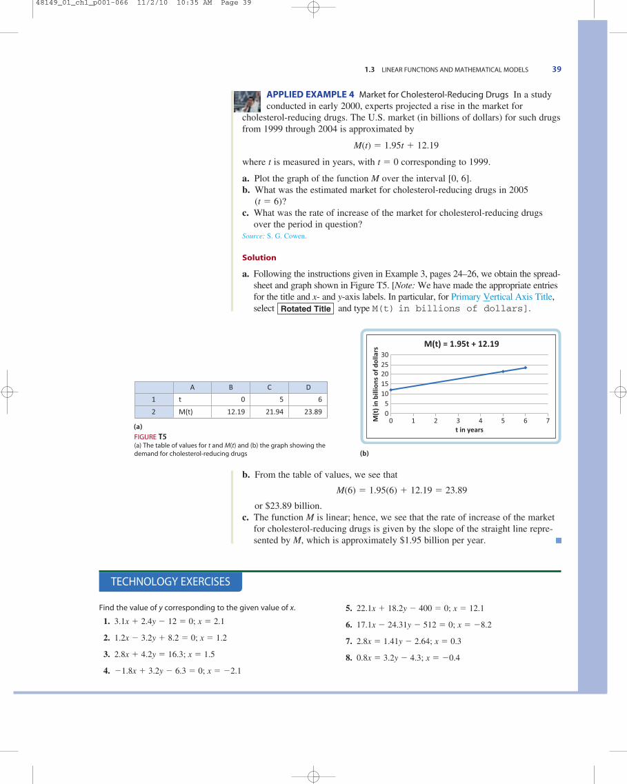
1.3 LINEAR FUNCTIONS AND MATHEMATICAL MODELS 39
APPLIED EXAMPLE 4 Market for Cholesterol-Reducing Drugs In a studyconducted in early 2000, experts projected a rise in the market for
cholesterol-reducing drugs. The U.S. market (in billions of dollars) for such drugsfrom 1999 through 2004 is approximated by
M(t) � 1.95t � 12.19
where t is measured in years, with t � 0 corresponding to 1999.
a. Plot the graph of the function M over the interval [0, 6].b. What was the estimated market for cholesterol-reducing drugs in 2005
(t � 6)?c. What was the rate of increase of the market for cholesterol-reducing drugs
over the period in question?Source: S. G. Cowen.
Solution
a. Following the instructions given in Example 3, pages 24–26, we obtain the spread-sheet and graph shown in Figure T5. [Note: We have made the appropriate entriesfor the title and x- and y-axis labels. In particular, for Primary Vertical Axis Title,select and type M(t) in billions of dollars].
b. From the table of values, we see that
M(6) � 1.95(6) � 12.19 � 23.89
or $23.89 billion.c. The function M is linear; hence, we see that the rate of increase of the market
for cholesterol-reducing drugs is given by the slope of the straight line repre-sented by M, which is approximately $1.95 billion per year.
Rotated Title
M(t) = 1.95t + 12.19
201510
5
3025
00 21 43
t in years
M(t
) in
billi
ons
of d
olla
rs
5 6 7
t 0
M(t) 12.192
1
21.94
5
A B C
23.89
6
D
FIGURE T5(a) The table of values for t and M(t) and (b) the graph showing thedemand for cholesterol-reducing drugs
TECHNOLOGY EXERCISES
Find the value of y corresponding to the given value of x.
1. 3.1x � 2.4y � 12 � 0; x � 2.1
2. 1.2x � 3.2y � 8.2 � 0; x � 1.2
3. 2.8x � 4.2y � 16.3; x � 1.5
4. �1.8x � 3.2y � 6.3 � 0; x � �2.1
5. 22.1x � 18.2y � 400 � 0; x � 12.1
6. 17.1x � 24.31y � 512 � 0; x � �8.2
7. 2.8x � 1.41y � 2.64; x � 0.3
8. 0.8x � 3.2y � 4.3; x � �0.4
(a)
(b)
48149_01_ch1_p001-066 11/2/10 10:35 AM Page 39

40 CHAPTER 1 STRAIGHT LINES AND LINEAR FUNCTIONS
Finding the Point of Intersection
The solution of certain practical problems involves finding the point of intersection oftwo straight lines. To see how such a problem may be solved algebraically, supposewe are given two straight lines L1 and L2 with equations
y � m1x � b1 and y � m2x � b2
(where m1, b1, m2, and b2 are constants) that intersect at the point P(x0, y0) (Figure 35).The point P(x0, y0) lies on the line L1, so it satisfies the equation y � m1x � b1. It
also lies on the line L2, so it satisfies the equation y � m2x � b2. Therefore, to find thepoint of intersection P(x0, y0) of the lines L1 and L2, we solve the system composed ofthe two equations
y � m1x � b1 and y � m2x � b2
for x and y.
EXAMPLE 1 Find the point of intersection of the straight lines that have equations y � x � 1 and y � �2x � 4.
Solution We solve the given simultaneous equations. Substituting the value y asgiven in the first equation into the second, we obtain
Substituting this value of x into either one of the given equations yields y � 2.Therefore, the required point of intersection is (1, 2) (Figure 36).
We now turn to some applications involving the intersections of pairs of straightlines.
Break-Even Analysis
Consider a firm with (linear) cost function C(x), revenue function R(x), and profitfunction P(x) given by
P1x 2 � R1x 2 � C1x 2 � 1s � c 2x � F
R1x 2 � sx
C1x 2 � cx � F
x � 1
3x � 3
x � 1 � �2x � 4
x5
y
5
–5
(1, 2)
y = –2x + 4 y = x + 1
L1L2
FIGURE 36The point of intersection of L1 and L2 is (1, 2).
x
y
L1
P(x0, y0)
L2
FIGURE 35L1 and L2 intersect at the point P(x0, y0).
1.4 Intersection of Straight Lines
Exploring withTECHNOLOGY
1. Use a graphing utility to plot the straight lines L1 and L2 with equations y � 3x � 2 and y � �2x � 3, respectively, on the same set of axes in the standard viewing window. Then use TRACE and ZOOM to find the point ofintersection of L1 and L2. Repeat using the “intersection” function of yourgraphing utility.
2. Find the point of intersection of L1 and L2 algebraically.
3. Comment on the effectiveness of each method.
VIDEO
48149_01_ch1_p001-066 11/2/10 10:35 AM Page 40
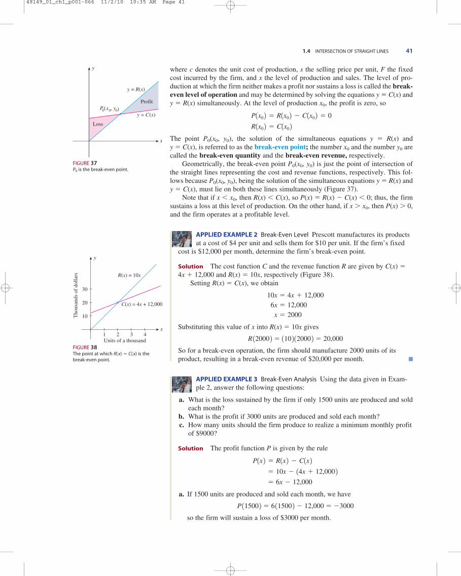
where c denotes the unit cost of production, s the selling price per unit, F the fixedcost incurred by the firm, and x the level of production and sales. The level of pro-duction at which the firm neither makes a profit nor sustains a loss is called the break-even level of operation and may be determined by solving the equations y � C(x) andy � R(x) simultaneously. At the level of production x0, the profit is zero, so
The point P0(x0, y0), the solution of the simultaneous equations y � R(x) and y � C(x), is referred to as the break-even point; the number x0 and the number y0 arecalled the break-even quantity and the break-even revenue, respectively.
Geometrically, the break-even point P0(x0, y0) is just the point of intersection ofthe straight lines representing the cost and revenue functions, respectively. This fol-lows because P0(x0, y0), being the solution of the simultaneous equations y � R(x) andy � C(x), must lie on both these lines simultaneously (Figure 37).
Note that if x � x0, then R(x) � C(x), so P(x) � R(x) � C(x) � 0; thus, the firmsustains a loss at this level of production. On the other hand, if x � x0, then P(x) � 0,and the firm operates at a profitable level.
APPLIED EXAMPLE 2 Break-Even Level Prescott manufactures its productsat a cost of $4 per unit and sells them for $10 per unit. If the firm’s fixed
cost is $12,000 per month, determine the firm’s break-even point.
Solution The cost function C and the revenue function R are given by C(x) �4x � 12,000 and R(x) � 10x, respectively (Figure 38).
Setting R(x) � C(x), we obtain
Substituting this value of x into R(x) � 10x gives
R 12000 2 � 110 2 12000 2 � 20,000
So for a break-even operation, the firm should manufacture 2000 units of itsproduct, resulting in a break-even revenue of $20,000 per month.
APPLIED EXAMPLE 3 Break-Even Analysis Using the data given in Exam-ple 2, answer the following questions:
a. What is the loss sustained by the firm if only 1500 units are produced and soldeach month?
b. What is the profit if 3000 units are produced and sold each month?c. How many units should the firm produce to realize a minimum monthly profit
of $9000?
Solution The profit function P is given by the rule
a. If 1500 units are produced and sold each month, we have
P 11500 2 � 6 11500 2 � 12,000 � �3000
so the firm will sustain a loss of $3000 per month.
� 6x � 12,000
� 10x � 14x � 12,000 2P1x 2 � R1x 2 � C1x 2
x � 2000 6x � 12,000
10x � 4x � 12,000
R1x0 2 � C1x0 2P1x0 2 � R1x0 2 � C1x0 2 � 0
1.4 INTERSECTION OF STRAIGHT LINES 41
x
y
y = R(x)
y = C(x)P0(x0, y0)
Profit
Loss
FIGURE 37P0 is the break-even point.
x1 2 3 4
y
30
20
10Tho
usan
ds o
f do
llars
Units of a thousand
C(x) = 4x + 12,000
R(x) = 10x
FIGURE 38The point at which R( x) � C( x) is thebreak-even point.
48149_01_ch1_p001-066 11/2/10 10:35 AM Page 41

b. If 3000 units are produced and sold each month, we have
P 13000 2 � 6 13000 2 � 12,000 � 6000
or a monthly profit of $6000.c. Substituting 9000 for P(x) in the equation P(x) � 6x � 12,000, we obtain
Thus, the firm should produce at least 3500 units to realize a $9000 minimummonthly profit.
APPLIED EXAMPLE 4 Decision Analysis The management of RobertsonControls must decide between two manufacturing processes for its model C
electronic thermostat. The monthly cost of the first process is given by C1(x) �20x � 10,000 dollars, where x is the number of thermostats produced; themonthly cost of the second process is given by C2(x) � 10x � 30,000 dollars. Ifthe projected monthly sales are 800 thermostats at a unit price of $40, whichprocess should management choose in order to maximize the company’s profit?
Solution The break-even level of operation using the first process is obtainedby solving the equation
giving an output of 500 units. Next, we solve the equation
giving an output of 1000 units for a break-even operation using the secondprocess. Since the projected sales are 800 units, we conclude that managementshould choose the first process, which will give the firm a profit.
APPLIED EXAMPLE 5 Decision Analysis Referring to Example 4, decidewhich process Robertson’s management should choose if the projected
monthly sales are (a) 1500 units and (b) 3000 units.
Solution In both cases, the production is past the break-even level. Since therevenue is the same regardless of which process is employed, the decision will bebased on how much each process costs.
a. If x � 1500, then
Hence, management should choose the first process.b. If x � 3000, then
In this case, management should choose the second process.
C21x 2 � 110 2 13000 2 � 30,000 � 60,000
C11x 2 � 120 2 13000 2 � 10,000 � 70,000
C21x 2 � 110 2 11500 2 � 30,000 � 45,000
C11x 2 � 120 2 11500 2 � 10,000 � 40,000
x � 1000
30x � 30,000
40x � 10x � 30,000
x � 500
20x � 10,000
40x � 20x � 10,000
x � 3500
6x � 21,000
9000 � 6x � 12,000
42 CHAPTER 1 STRAIGHT LINES AND LINEAR FUNCTIONS
48149_01_ch1_p001-066 11/2/10 10:35 AM Page 42

Market Equilibrium
Under pure competition, the price of a commodity eventually settles at a level dic-tated by the condition that the supply of the commodity be equal to the demand for it. If the price is too high, consumers will be more reluctant to buy, and if theprice is too low, the supplier will be more reluctant to make the product availablein the marketplace. Market equilibrium is said to prevail when the quantity pro-duced is equal to the quantity demanded. The quantity produced at market equilib-rium is called the equilibrium quantity, and the corresponding price is called theequilibrium price.
From a geometric point of view, market equilibrium corresponds to the point atwhich the demand curve and the supply curve intersect. In Figure 39, x0 represents theequilibrium quantity and p0 the equilibrium price. The point (x0, p0) lies on the supplycurve and therefore satisfies the supply equation. At the same time, it also lies on thedemand curve and therefore satisfies the demand equation. Thus, to find the point (x0, p0), and hence the equilibrium quantity and price, we solve the demand and sup-ply equations simultaneously for x and p. For meaningful solutions, x and p must bothbe positive.
APPLIED EXAMPLE 6 Market Equilibrium The management of Thermo-Master, which manufactures an indoor–outdoor thermometer at its Mexico
subsidiary, has determined that the demand equation for its product is
5x � 3p � 30 � 0
where p is the price of a thermometer in dollars and x is the quantity demanded in units of a thousand. The supply equation for these thermometers is
52x � 30p � 45 � 0
where x (measured in thousands) is the quantity that ThermoMaster will makeavailable in the market at p dollars each. Find the equilibrium quantity and price.
Solution We need to solve the system of equations
for x and p. Let us use the method of substitution to solve it. As the name sug-gests, this method calls for choosing one of the equations in the system, solving
52x � 30p � 45 � 0
5x � 3p � 30 � 0
1.4 INTERSECTION OF STRAIGHT LINES 43
Exploring withTECHNOLOGY
1. Use a graphing utility to plot the straight lines L1 and L2 with equations y � 2x � 1 and y � 2.1x � 3, respectively, on the same set of axes, using thestandard viewing window. Do the lines appear to intersect?
2. Plot the straight lines L1 and L2, using the viewing window [�100, 100] �[�100, 100]. Do the lines appear to intersect? Can you find the point of inter-section using TRACE and ZOOM? Using the “intersection” function of yourgraphing utility?
3. Find the point of intersection of L1 and L2 algebraically.
4. Comment on the effectiveness of the solution methods in parts 2 and 3.
xx0
p
p0 (x0, p0)
Demand curve
Supply curve
FIGURE 39Market equilibrium is represented by thepoint (x0, p0).
48149_01_ch1_p001-066 11/2/10 10:35 AM Page 43
for one variable in terms of the other, and then substituting the resulting expres-sion into the other equation. This gives an equation in one variable that can thenbe solved in the usual manner.
Let’s solve the first equation for p in terms of x. Thus,
Next, we substitute this value of p into the second equation, obtaining
The corresponding value of p is found by substituting this value of x into theequation for p obtained earlier. Thus,
We conclude that the equilibrium quantity is 2500 units (remember that x is mea-sured in units of a thousand) and the equilibrium price is $5.83 per thermometer.
APPLIED EXAMPLE 7 Market Equilibrium The quantity demanded of a cer-tain model of DVD player is 8000 units when the unit price is $260. At a
unit price of $200, the quantity demanded increases to 10,000 units. The manu-facturer will not market any players if the price is $100 or lower. However, foreach $50 increase in the unit price above $100, the manufacturer will market anadditional 1000 units. Both the demand and the supply equations are known to belinear.
a. Find the demand equation.b. Find the supply equation.c. Find the equilibrium quantity and price.
Solution Let p denote the unit price in hundreds of dollars, and let x denote thenumber of units of players in thousands.
a. Since the demand function is linear, the demand curve is a straight line pass-ing through the points (8, 2.6) and (10, 2). Its slope is
Using the point (10, 2) and the slope m � �0.3 in the point-slope form of theequation of a line, we see that the required demand equation is
Figure 40 p � �0.3x � 5
p � 2 � �0.31x � 10 2
m �2 � 2.6
10 � 8� �0.3
�35
6� 5.83
p � �5
3a 5
2b � 10 � �
25
6� 10
x �255
102�
5
2
102x � 255 � 0
52x � 50x � 300 � 45 � 0
52x � 30 a�5
3 x � 10 b � 45 � 0
p � �5
3 x � 10
3p � �5x � 30
44 CHAPTER 1 STRAIGHT LINES AND LINEAR FUNCTIONS
VIDEO
48149_01_ch1_p001-066 11/2/10 10:35 AM Page 44

b. The supply curve is the straight line passing through the points (0, 1) and (1, 1.5). Its slope is
Using the point (0, 1) and the slope m � 0.5 in the point-slope form of theequation of a line, we see that the required supply equation is
Figure 40
c. To find the market equilibrium, we solve simultaneously the system compris-ing the demand and supply equations obtained in parts (a) and (b)—that is, thesystem
Subtracting the first equation from the second gives
0.8x � 4 � 0
and x � 5. Substituting this value of x in the second equation gives p � 3.5. Thus, the equilibrium quantity is 5000 units, and the equilibrium price is $350(Figure 40).
p � 0.5x � 1
p � �0.3x � 5
p � 0.5x � 1
p � 1 � 0.51x � 0 2
m �1.5 � 1
1 � 0� 0.5
x5
p
6
5
4
3
2
1
Units of a thousand
Uni
tpri
cein
hund
reds
ofdo
llars
p = 0.5x + 1
10 15 20
p = –0.3x + 5
(5, 3.5)
1.4 INTERSECTION OF STRAIGHT LINES 45
FIGURE 40Market equilibrium occurs at the point (5, 3.5).
p � 0.5x � 1�p � 0.3x � 5
0 � 0.8x � 4
1.4 Self-Check Exercises
1. Find the point of intersection of the straight lines withequations 2x � 3y � 6 and x � 3y � 4.
2. There is no demand for a certain model of a disposablecamera when the unit price is $12. However, when the unitprice is $8, the quantity demanded is 8000/week. The sup-pliers will not market any cameras if the unit price is $2 or lower. At $4/camera, however, the manufacturer will
market 5000 cameras/week. Both the demand and supplyfunctions are known to be linear.a. Find the demand equation.b. Find the supply equation.c. Find the equilibrium quantity and price.
Solutions to Self-Check Exercises 1.4 can be found on page 48.
48149_01_ch1_p001-066 11/2/10 10:35 AM Page 45

46 CHAPTER 1 STRAIGHT LINES AND LINEAR FUNCTIONS
1.4 Exercises
In Exercises 1–6, find the point of intersection of each pair ofstraight lines.
1. y � 3x � 4 2. y � �4x � 7y � �2x � 14 �y � 5x � 10
3. 2x � 3y � 6 4. 2x � 4y � 113x � 6y � 16 �5x � 3y � 5
5. 6.
x � 3y � 3 � 0
In Exercises 7–10, find the break-even point for the firm whosecost function C and revenue function R are given.
7. C 1x 2 � 5x � 10,000; R 1x 2 � 15x
8. C 1x 2 � 15x � 12,000; R 1x 2 � 21x
9. C 1x 2 � 0.2x � 120; R 1x 2 � 0.4x
10. C 1x 2 � 150x � 20,000; R 1x 2 � 270x
11. BREAK-EVEN ANALYSIS AutoTime, a manufacturer of 24-hrvariable timers, has a monthly fixed cost of $48,000 and aproduction cost of $8 for each timer manufactured. Theunits sell for $14 each.a. Sketch the graphs of the cost function and the reve-
nue function and thereby find the break-even pointgraphically.
b. Find the break-even point algebraically.c. Sketch the graph of the profit function.d. At what point does the graph of the profit function cross
the x-axis? Interpret your result.
12. BREAK-EVEN ANALYSIS A division of Carter Enterprisesproduces “Personal Income Tax” diaries. Each diary sellsfor $8. The monthly fixed costs incurred by the divisionare $25,000, and the variable cost of producing each diaryis $3.a. Find the break-even point for the division.b. What should be the level of sales in order for the divi-
sion to realize a 15% profit over the cost of making thediaries?
2x �3
2 y � 1
y �2
3 x � 4y �
1
4 x � 5
13. BREAK-EVEN ANALYSIS A division of the Gibson Corpor-ation manufactures bicycle pumps. Each pump sells for $9,and the variable cost of producing each unit is 40% of theselling price. The monthly fixed costs incurred by the divi-sion are $50,000. What is the break-even point for thedivision?
14. LEASING Ace Truck Leasing Company leases a certain sizetruck for $30/day and $.15/mi, whereas Acme Truck Leas-ing Company leases the same size truck for $25/day and$.20/mi.a. Find the functions describing the daily cost of leasing
from each company.b. Sketch the graphs of the two functions on the same set
of axes.c. If a customer plans to drive at most 70 mi, from which
company should he rent a truck for a single day?
15. DECISION ANALYSIS A product may be made by usingMachine I or Machine II. The manufacturer estimates thatthe monthly fixed costs of using Machine I are $18,000,whereas the monthly fixed costs of using Machine II are$15,000. The variable costs of manufacturing 1 unit of theproduct using Machine I and Machine II are $15 and $20,respectively. The product sells for $50 each.a. Find the cost functions associated with using each
machine.b. Sketch the graphs of the cost functions of part (a) and
the revenue functions on the same set of axes.c. Which machine should management choose in order to
maximize their profit if the projected sales are 450 units?550 units? 650 units?
d. What is the profit for each case in part (c)?
16. ANNUAL SALES The annual sales of Crimson Drug Store areexpected to be given by S � 2.3 � 0.4t million dollars t years from now, whereas the annual sales of CambridgeDrug Store are expected to be given by S � 1.2 � 0.6t mil-lion dollars t years from now. When will Cambridge’sannual sales first surpass Crimson’s annual sales?
1. Explain why you would expect that the intersection of alinear demand curve and a linear supply curve would liein the first quadrant.
2. Explain the meaning of each term:a. Break-even pointb. Break-even quantityc. Break-even revenue
3. Explain the meaning of each term:a. Market equilibriumb. Equilibrium quantityc. Equilibrium price
1.4 Concept Questions
48149_01_ch1_p001-066 11/2/10 10:35 AM Page 46
17. LCDs VERSUS CRTs The global shipments of traditionalcathode-ray tube monitors (CRTs) is approximated by theequation
y � �12t � 88 10 � t � 3 2where y is measured in millions and t in years, with t � 0corresponding to the beginning of 2001. The equation
y � 18t � 13.4 10 � t � 3 2gives the approximate number (in millions) of liquid crys-tal displays (LCDs) over the same period. When did theglobal shipments of LCDs first overtake the global ship-ments of CRTs?Source: International Data Corporation.
18. DIGITAL VERSUS FILM CAMERAS The sales of digital cameras(in millions of units) in year t is given by the function
f 1t 2 � 3.05t � 6.85 10 � t � 3 2where t � 0 corresponds to 2001. Over that same period,the sales of film cameras (in millions of units) is given by
t 1t 2 � �1.85t � 16.58 10 � t � 3 2a. Show that more film cameras than digital cameras were
sold in 2001.b. When did the sales of digital cameras first exceed those
of film cameras?Source: Popular Science.
19. U.S. FINANCIAL TRANSACTIONS The percentage of U.S. trans-actions by check between the beginning of 2001 (t � 0) andthe beginning of 2010 (t � 9) is approximated by
whereas the percentage of transactions done electronicallyduring the same period is approximated by
a. Sketch the graphs of f and t on the same set of axes.b. Find the time when transactions done electronically first
exceeded those done by check.Source: Foreign Policy.
20. BROADBAND VERSUS DIAL-UP The number of U.S. broadbandInternet households (in millions) between the beginning of2004 (t � 0) and the beginning of 2008 (t � 4) is approxi-mated by
f 1t 2 � 6.5t � 33 10 � t � 4 2Over the same period, the number of U.S. dial-up Internethouseholds (in millions) is approximated by
t 1t 2 � �3.9t � 42.5 10 � t � 4 2a. Sketch the graphs of f and t on the same set of axes.b. Solve the equation f (t) � t(t), and interpret your result.Source: Strategic Analytics, Inc.
t1t 2 �11
3 t � 23 10 � t � 9 2
f 1t 2 � �11
9 t � 43 10 � t � 9 2
1.4 INTERSECTION OF STRAIGHT LINES 47
For each pair of supply-and-demand equations in Exercises21–24, where x represents the quantity demanded in units of1000 and p is the unit price in dollars, find the equilibrium quan-tity and the equilibrium price.
21. 4x � 3p � 59 � 0 and 5x � 6p � 14 � 0
22. 2x � 7p � 56 � 0 and 3x � 11p � 45 � 0
23. p � �2x � 22 and p � 3x � 12
24. p � �0.3x � 6 and p � 0.15x � 1.5
25. EQUILIBRIUM QUANTITY AND PRICE The quantity demanded ofa certain brand of DVD player is 3000/week when the unitprice is $485. For each decrease in unit price of $20 below$485, the quantity demanded increases by 250 units. Thesuppliers will not market any DVD players if the unit priceis $300 or lower. But at a unit price of $525, they are will-ing to make available 2500 units in the market. The supplyequation is also known to be linear.a. Find the demand equation.b. Find the supply equation.c. Find the equilibrium quantity and price.
26. EQUILIBRIUM QUANTITY AND PRICE The demand equation forthe Drake GPS Navigator is x � 4p � 800 � 0, where x isthe quantity demanded per week and p is the wholesale unitprice in dollars. The supply equation is x � 20p � 1000 �0, where x is the quantity the supplier will make availablein the market each week when the wholesale price is p dol-lars each. Find the equilibrium quantity and the equilib-rium price for the GPS Navigators.
27. EQUILIBRIUM QUANTITY AND PRICE The demand equation forthe Schmidt-3000 fax machine is 3x � p � 1500 � 0,where x is the quantity demanded per week and p is the unitprice in dollars. The supply equation is 2 x � 3p � 1200 �0, where x is the quantity the supplier will make availablein the market each week when the unit price is p dollars.Find the equilibrium quantity and the equilibrium price forthe fax machines.
28. EQUILIBRIUM QUANTITY AND PRICE The quantity demandedeach month of Russo Espresso Makers is 250 when theunit price is $140; the quantity demanded each month is 1000 when the unit price is $110. The suppliers willmarket 750 espresso makers if the unit price is $60 orhigher. At a unit price of $80, they are willing to market2250 units. Both the demand and supply equations areknown to be linear.a. Find the demand equation.b. Find the supply equation.c. Find the equilibrium quantity and the equilibrium price.
29. Suppose the demand and supply equations for a certaincommodity are given by p � ax � b and p � cx � d,respectively, where a � 0, c � 0, and b � d � 0 (see thefollowing figure).
48149_01_ch1_p001-066 11/2/10 10:35 AM Page 47
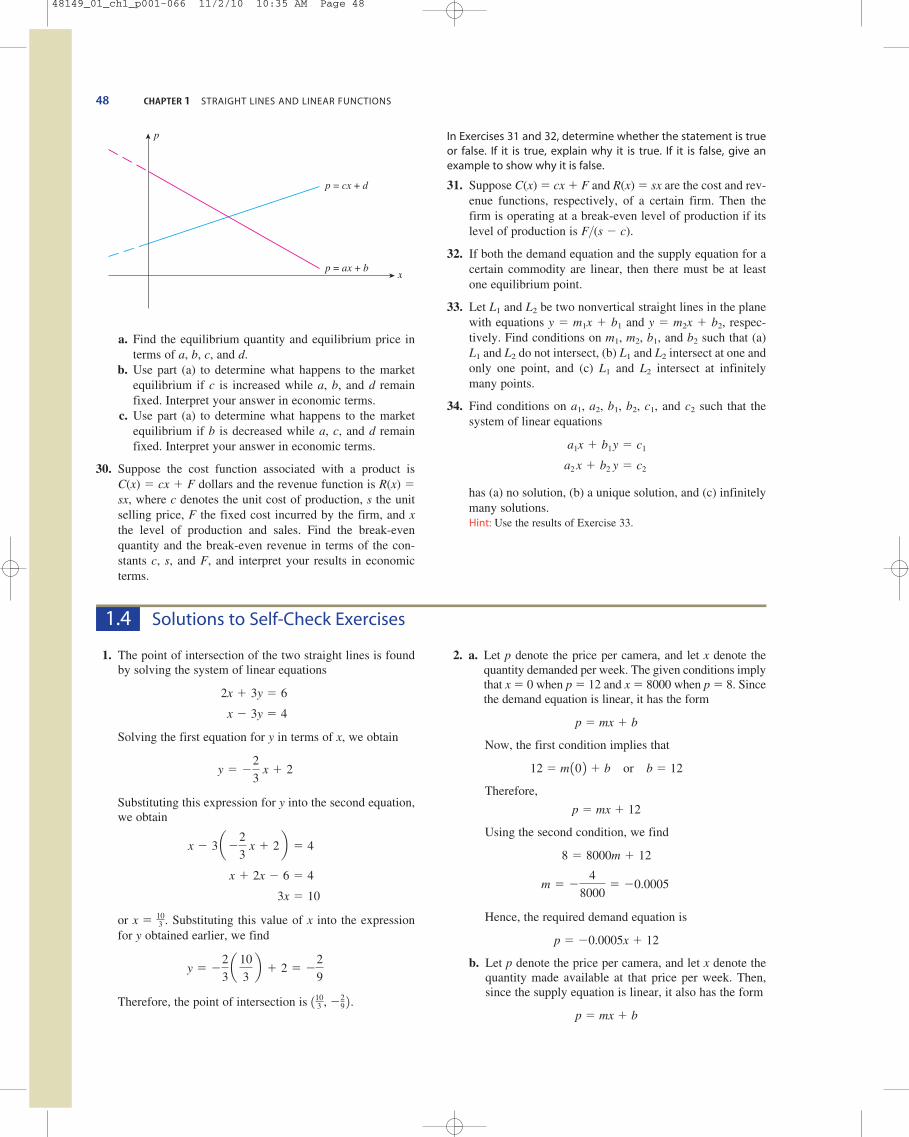
48 CHAPTER 1 STRAIGHT LINES AND LINEAR FUNCTIONS
a. Find the equilibrium quantity and equilibrium price interms of a, b, c, and d.
b. Use part (a) to determine what happens to the marketequilibrium if c is increased while a, b, and d remainfixed. Interpret your answer in economic terms.
c. Use part (a) to determine what happens to the marketequilibrium if b is decreased while a, c, and d remainfixed. Interpret your answer in economic terms.
30. Suppose the cost function associated with a product is C(x) � cx � F dollars and the revenue function is R(x) �sx, where c denotes the unit cost of production, s the unitselling price, F the fixed cost incurred by the firm, and xthe level of production and sales. Find the break-evenquantity and the break-even revenue in terms of the con-stants c, s, and F, and interpret your results in economicterms.
x
p
p = cx + d
p = ax + b
1. The point of intersection of the two straight lines is foundby solving the system of linear equations
Solving the first equation for y in terms of x, we obtain
Substituting this expression for y into the second equation,we obtain
or . Substituting this value of x into the expressionfor y obtained earlier, we find
Therefore, the point of intersection is .1103 , �2
9 2y � �
2
3a 10
3b � 2 � �
2
9
x � 103
3x � 10
x � 2x � 6 � 4
x � 3 a�2
3 x � 2 b � 4
y � �2
3 x � 2
x � 3y � 4
2x � 3y � 6
In Exercises 31 and 32, determine whether the statement is trueor false. If it is true, explain why it is true. If it is false, give anexample to show why it is false.
31. Suppose C(x) � cx � F and R(x) � sx are the cost and rev-enue functions, respectively, of a certain firm. Then thefirm is operating at a break-even level of production if itslevel of production is F>(s � c).
32. If both the demand equation and the supply equation for acertain commodity are linear, then there must be at leastone equilibrium point.
33. Let L1 and L2 be two nonvertical straight lines in the planewith equations y � m1x � b1 and y � m2x � b2, respec-tively. Find conditions on m1, m2, b1, and b2 such that (a)L1 and L2 do not intersect, (b) L1 and L2 intersect at one andonly one point, and (c) L1 and L2 intersect at infinitelymany points.
34. Find conditions on a1, a2, b1, b2, c1, and c2 such that thesystem of linear equations
has (a) no solution, (b) a unique solution, and (c) infinitelymany solutions.Hint: Use the results of Exercise 33.
a2 x � b2
y � c2
a1x � b1 y � c1
2. a. Let p denote the price per camera, and let x denote thequantity demanded per week. The given conditions implythat x � 0 when p � 12 and x � 8000 when p � 8. Sincethe demand equation is linear, it has the form
p � mx � b
Now, the first condition implies that
12 � m 10 2 � b or b � 12
Therefore,
p � mx � 12
Using the second condition, we find
Hence, the required demand equation is
p � �0.0005x � 12
b. Let p denote the price per camera, and let x denote thequantity made available at that price per week. Then,since the supply equation is linear, it also has the form
p � mx � b
m � �4
8000� �0.0005
8 � 8000m � 12
1.4 Solutions to Self-Check Exercises
48149_01_ch1_p001-066 11/2/10 10:35 AM Page 48

1.4 INTERSECTION OF STRAIGHT LINES 49
Finding the Point(s) of Intersection of Two Graphs
Graphing UtilityA graphing utility can be used to find the point(s) of intersection of the graphs of two functions. Once again, it is important to remember that if the graphs are straightlines, the linear equations defining these lines must first be recast in the slope-interceptform.
EXAMPLE 1 Find the points of intersection of the straight lines with equations 2x � 3y � 6 and 3x � 4y � 5 � 0.
Solution Method I Solving each equation for y in terms of x, we obtain
as the respective equations in the slope-intercept form. The graphs of the twostraight lines in the standard viewing window are shown in Figure T1.
Then, using TRACE and ZOOM or the function for finding the point of intersec-tion of two graphs, we find that the point of intersection, accurate to four decimalplaces, is (2.2941, 0.4706).
Method II Proceed as before to obtain the graphs of the two lines. Then use theintersect function of the graphing utility to find the point of intersection, (2.2941176,0.47058824), of the two straight lines (Figure T2).
Note On the TI-83/84, you can call the intersect function by selecting the CALC menuand then selecting 5: intersect (Figure T3a). Press to obtain the graphENTER
y � �2
3 x � 2 and y �
3
4 x �
5
4
USINGTECHNOLOGY
(continued)
The first condition implies that x � 0 when p � 2, sowe have
2 � m 10 2 � b or b � 2
Therefore,
p � mx � 2
Next, using the second condition, x � 5000 when p � 4,we find
4 � 5000m � 2
giving m � 0.0004. So the required supply equation is
p � 0.0004x � 2
c. The equilibrium quantity and price are found by solvingthe system of linear equations
Equating the two expressions yields
or x � 11,111. Substituting this value of x into eitherequation in the system yields
p � 6.44
Therefore, the equilibrium quantity is 11,111, and theequilibrium price is $6.44.
0.0009x � 10
�0.0005x � 12 � 0.0004x � 2
p � 0.0004x � 2
p � �0.0005x � 12
10
_10
10_10
FIGURE T1The straight lines 2x � 3y � 6 and 3x � 4y � 5 � 0
IntersectionX=2.2941176 Y=.47058824FIGURE T2
48149_01_ch1_p001-066 11/3/10 11:36 AM Page 49
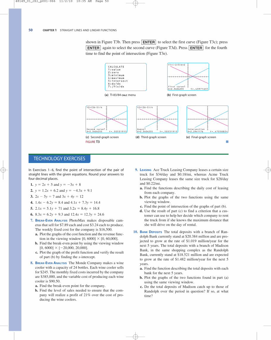
50 CHAPTER 1 STRAIGHT LINES AND LINEAR FUNCTIONS
shown in Figure T3b. Then press to select the first curve (Figure T3c); pressagain to select the second curve (Figure T3d). Press for the fourth
time to find the point of intersection (Figure T3e).
(a) TI-83/84 CALC menu (b) First-graph screen
ENTERENTER
ENTER
CALCULATE1:value2:zero3:minimum4:maximum5:intersect6:dy/dx7: f(x)dx
FIGURE T3
First curve?X=2.3404255 Y=.43971631
Y1=(–2/3)X+2
Second curve?X=2.3404255 Y=.50531915
Y2=(3X–5)/4
Guess?X=2.3404255 Y=.50531915
Y2=(3X–5)/4
IntersectionX=2.2941176 Y=.47058824
(c) Second-graph screen (d) Third-graph screen (e) Final-graph screen
In Exercises 1–6, find the point of intersection of the pair ofstraight lines with the given equations. Round your answers tofour decimal places.
1. y � 2x � 5 and y � �3x � 8
2. y � 1.2x � 6.2 and y � �4.3x � 9.1
3. 2x � 5y � 7 and 3x � 4y � 12
4. 1.4x � 6.2y � 8.4 and 4.1x � 7.3y � 14.4
5. 2.1x � 5.1y � 71 and 3.2x � 8.4y � 16.8
6. 8.3x � 6.2y � 9.3 and 12.4x � 12.3y � 24.6
7. BREAK-EVEN ANALYSIS PhotoMax makes disposable cam-eras that sell for $7.89 each and cost $3.24 each to produce.The weekly fixed cost for the company is $16,500.a. Plot the graphs of the cost function and the revenue func-
tion in the viewing window [0, 6000] � [0, 60,000].b. Find the break-even point by using the viewing window
[0, 6000] � [�20,000, 20,000].c. Plot the graph of the profit function and verify the result
of part (b) by finding the x-intercept.
8. BREAK-EVEN ANALYSIS The Monde Company makes a winecooler with a capacity of 24 bottles. Each wine cooler sellsfor $245. The monthly fixed costs incurred by the companyare $385,000, and the variable cost of producing each winecooler is $90.50.a. Find the break-even point for the company.b. Find the level of sales needed to ensure that the com-
pany will realize a profit of 21% over the cost of pro-ducing the wine coolers.
9. LEASING Ace Truck Leasing Company leases a certain sizetruck for $34/day and $0.18/mi, whereas Acme TruckLeasing Company leases the same size truck for $28/dayand $0.22/mi.a. Find the functions describing the daily cost of leasing
from each company.b. Plot the graphs of the two functions using the same
viewing window.c. Find the point of intersection of the graphs of part (b).d. Use the result of part (c) to find a criterion that a cus-
tomer can use to help her decide which company to rentthe truck from if she knows the maximum distance thatshe will drive on the day of rental.
10. BANK DEPOSITS The total deposits with a branch of Ran-dolph Bank currently stand at $20.384 million and are pro-jected to grow at the rate of $1.019 million/year for thenext 5 years. The total deposits with a branch of MadisonBank, in the same shopping complex as the RandolphBank, currently stand at $18.521 million and are expectedto grow at the rate of $1.482 million/year for the next 5years.a. Find the function describing the total deposits with each
bank for the next 5 years.b. Plot the graphs of the two functions found in part (a)
using the same viewing window.c. Do the total deposits of Madison catch up to those of
Randolph over the period in question? If so, at whattime?
TECHNOLOGY EXERCISES
48149_01_ch1_p001-066 11/2/10 10:35 AM Page 50
1.5 THE METHOD OF LEAST SQUARES 51
1.5 The Method of Least Squares
The Method of Least Squares
In Example 10, Section 1.2, we saw how a linear equation may be used to approxi-mate the sales trend for a local sporting goods store. The trend line, as we saw, maybe used to predict the store’s future sales. Recall that we obtained the trend line inExample 10 by requiring that the line pass through two data points, the rationale beingthat such a line seems to fit the data reasonably well.
In this section, we describe a general method known as the method of leastsquares for determining a straight line that, in some sense, best fits a set of data pointswhen the points are scattered about a straight line. To illustrate the principle behindthe method of least squares, suppose, for simplicity, that we are given five data points,
P1 1x1, y1 2, P2 1x2, y2 2, P3 1x3, y3 2, P4 1x4, y4 2, P5 1x5, y5 2describing the relationship between the two variables x and y. By plotting these datapoints, we obtain a graph called a scatter diagram (Figure 41).
If we try to fit a straight line to these data points, the line will miss the first, sec-ond, third, fourth, and fifth data points by the amounts d1, d2, d3, d4, and d5, respec-tively (Figure 42). We can think of the amounts d1, d2, . . . , d5 as the errors made whenthe values y1, y2, . . . , y5 are approximated by the corresponding values of y lying onthe straight line L.
11. EQUILIBRIUM QUANTITY AND PRICE The quantity demanded ofa certain brand of a smart phone is 2000/week when theunit price is $84. For each decrease in unit price of $5below $84, the quantity demanded increases by 50 units.The supplier will not market any of the smart phones if theunit price is $60 or less, but the supplier will market1800/week if the unit price is $90. The supply equation isalso known to be linear.a. Find the demand and supply equations.b. Plot the graphs of the supply and demand equations and
find their point of intersection.c. Find the equilibrium quantity and price.
12. EQUILIBRIUM QUANTITY AND PRICE The demand equation for the Miramar Heat Machine, a ceramic heater, is 1.1x � 3.8p � 901 � 0, where x is the quantity demandedeach week and p is the wholesale unit price in dollars. Thecorresponding supply equation is 0.9x � 20.4p � 1038 �0, where x is the quantity the supplier will make availablein the market when the wholesale price is p dollars each.a. Plot the graphs of the demand and supply equations
using the same viewing window.b. Find the equilibrium quantity and the equilibrium price
for the Miramar heaters.
x5
y
10
5
P1
10
P2
P3
P4
P5
FIGURE 41A scatter diagram
x5
y
10
5
d1
10
d2
d3
d4
d5
FIGURE 42di is the vertical distance between the straightline and a given data point.
48149_01_ch1_p001-066 11/2/10 10:35 AM Page 51

The Method of Least Squares
Suppose we are given n data points
P1 1x1, y1 2, P2 1x2, y2 2, P3 1x3, y3 2, . . . , Pn 1xn, yn 2Then the least-squares (regression) line for the data is given by the linear equa-tion (function)
y � f 1x 2 � mx � b
where the constants m and b satisfy the normal equations
(9)
(10)
simultaneously.
� x1 y1 � x2
y2 � p � xn yn
1x1 � x2 � p � xn 2b � 1x21 � x2
2 � p � x2n 2m
nb � 1x1 � x2 � p � xn 2m � y1 � y2 � p � yn
52 CHAPTER 1 STRAIGHT LINES AND LINEAR FUNCTIONS
The principle of least squares states that the straight line L that fits the data pointsbest is the one chosen by requiring that the sum of the squares of d1, d2, . . . , d5—that is,
be made as small as possible. In other words, the least-squares criterion calls for min-imizing the sum of the squares of the errors. The line L obtained in this manner iscalled the least-squares line, or regression line.
The method for computing the least-squares lines that best fits a set of data pointsis contained in the following result, which we state without proof.
d21 � d2
2 � d23 � d2
4 � d25
PORTFOLIO
A Rich Experience Massage &Wellness Spa takes an integrativeapproach to health-related ser-vices in a modern spa environ-
ment. The spa provides a variety of services including mas-sage therapy, spa facials and body treatments, Bowenwork,hypnotherapy, and chiropractic care. A Rich Experience alsosells retail products and offers continuing education work-shops for massage therapists.
As an owner, I closely evaluate the company’s fixed andvariable revenue streams—generated from our beauty andspa services, retail sales, workshops, and rental space—todetermine if I am on track to meet my profitability goals. Iplot data points for all the revenue streams and apply theleast squares method to see if the best fit line matches myprofitability goals. This method allows me to see howincreases in specific revenue streams might affect overallprofitability.
Bodywork and Spa Services provide us with our mostprofitable revenue stream, so I try to maximize the numberof these services that we can provide. Based on our availablerooms and practitioners, we can provide 60 one-hour ser-vices per week. At an average of $70 per service, this equals$4200 per week or approximately $218,440 per year. In orderto gross $109,220 and meet my goals for net profitability,after one year the spa needs to be booking at least 50% ofour available time slots. My commissioned practitioners earn40% on all services they provide, so at 50% productivity, thisbrings my net total for Beauty and Spa Services to $65,532.
Applying my college mathematics and accountingcourses has helped me create a thriv-ing business. With additional market-ing efforts, name recognition, and apositive reputation in the community,I can anticipate that our bookings willcontinue to increase each year.
Melissa Rich
TITLE OwnerINSTITUTION A Rich Experience Massage & Wellness Spa
Courtesy of A Rich Experience; (inset) © Szasz-Fabian Ilka Erica/Shutterstock.com
48149_01_ch1_p001-066 11/2/10 10:35 AM Page 52
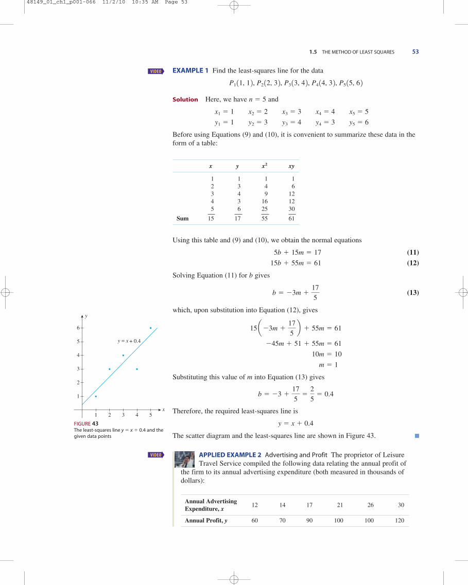
1.5 THE METHOD OF LEAST SQUARES 53
EXAMPLE 1 Find the least-squares line for the data
P1 11, 1 2, P2 12, 3 2, P3 13, 4 2, P4 14, 3 2, P5 15, 6 2Solution Here, we have n � 5 and
x1 � 1 x2 � 2 x3 � 3 x4 � 4 x5 � 5
y1 � 1 y2 � 3 y3 � 4 y4 � 3 y5 � 6
Before using Equations (9) and (10), it is convenient to summarize these data in theform of a table:
x y x2 xy
1 1 1 12 3 4 63 4 9 124 3 16 125 6 25 30
Sum 15 17 55 61
Using this table and (9) and (10), we obtain the normal equations
(11)
(12)
Solving Equation (11) for b gives
(13)
which, upon substitution into Equation (12), gives
Substituting this value of m into Equation (13) gives
Therefore, the required least-squares line is
y � x � 0.4
The scatter diagram and the least-squares line are shown in Figure 43.
APPLIED EXAMPLE 2 Advertising and Profit The proprietor of LeisureTravel Service compiled the following data relating the annual profit of
the firm to its annual advertising expenditure (both measured in thousands of dollars):
Annual Advertising12 14 17 21 26 30
Expenditure, x
Annual Profit, y 60 70 90 100 100 120
b � �3 �17
5�
2
5� 0.4
m � 1
10m � 10
�45m � 51 � 55m � 61
15 a�3m �17
5b � 55m � 61
b � �3m �17
5
15b � 55m � 61
5b � 15m � 17
x1 2 3 4 5
y
6
5
4
3
2
1
y = x + 0.4
FIGURE 43The least-squares line y � x � 0.4 and thegiven data points
VIDEO
VIDEO
48149_01_ch1_p001-066 11/2/10 10:35 AM Page 53

54 CHAPTER 1 STRAIGHT LINES AND LINEAR FUNCTIONS
a. Determine the equation of the least-squares line for these data.b. Draw a scatter diagram and the least-squares line for these data.c. Use the result obtained in part (a) to predict Leisure Travel’s annual profit if
the annual advertising budget is $20,000.
Solution
a. The calculations required for obtaining the normal equations are summarizedin the following table:
x y x2 xy
12 60 144 72014 70 196 98017 90 289 1,53021 100 441 2,10026 100 676 2,60030 120 900 3,600
Sum 120 540 2646 11,530
The normal equations are
(14)
(15)
Solving Equation (14) for b gives
b � �20m � 90 (16)
which, upon substitution into Equation (15), gives
Substituting this value of m into Equation (16) gives
Therefore, the required least-squares line is given by
y � f 1x 2 � 2.97x � 30.6
b. The scatter diagram and the least-squares line are shown in Figure 44.c. Leisure Travel’s predicted annual profit corresponding to an annual budget of
$20,000 is given by
f 120 2 � 2.97 120 2 � 30.6 � 90
or $90,000.
APPLIED EXAMPLE 3 U.S. Health-Care Expenditures Refer to Example 1 ofSection 1.3. Because the over-65 population will be growing more rapidly
in the next few decades, health-care spending is expected to increase significantlyin the coming decades. The following table gives the U.S. health expenditures (intrillions of dollars) from 2008 through 2013, where t is measured in years, with t � 0 corresponding to 2008.
b � �2012.97 2 � 90 � 30.6
m � 2.97
246m � 730
�2400m � 10,800 � 2646m � 11,530
1201�20m � 90 2 � 2646m � 11,530
120b � 2646m � 11,530
6b � 120m � 540
x5
y
100
50
y = 2.97x + 30.6
10 15 Thousands of dollars
Tho
usan
ds o
f do
llars
20 25 30
FIGURE 44Profit versus advertising expenditure
48149_01_ch1_p001-066 11/2/10 10:35 AM Page 54

Year, t 0 1 2 3 4 5
Expenditure, y 2.34 2.47 2.57 2.70 2.85 3.02
(The figures after 2009 are estimates.) Find a function giving the U.S. health-carespending between 2008 and 2013, using the least-squares technique.Source: Centers for Medicare & Medicaid Services.
Solution The calculations required for obtaining the normal equations are sum-marized in the following table:
t y t2 ty
0 2.34 0 01 2.47 1 2.472 2.57 4 5.143 2.70 9 8.104 2.85 16 11.405 3.02 25 15.10
15 15.95 55 42.21
The normal equations are
(17)
(18)
Solving Equation (17) for b gives
b � �2.5m � 2.6583 (19)
which, upon substitution into Equation (18), gives
Substituting this value of m into Equation (19) gives
b � �2.5 10.13352 � 2.6583 � 2.3246
Therefore, the required function is
S 1t 2 � 0.134t � 2.325
m � 0.1335
17.5m � 2.3355
�37.5m � 39.8745 � 55m � 42.21
151�2.5m � 2.6583 2 � 55m � 42.21
15b � 55m � 42.21
6b � 15m � 15.95
1.5 THE METHOD OF LEAST SQUARES 55
1.5 Self-Check Exercises
1. Find an equation of the least-squares line for the data
x 1 3 4 5 7
y 4 10 11 12 16
2. In a market research study for Century Communications,the following data were provided based on the projectedmonthly sales x (in thousands) of a DVD version of a box-office-hit adventure movie with a proposed wholesale unitprice of p dollars.
x 2.2 5.4 7.0 11.5 14.6
p 38.0 36.0 34.5 30.0 28.5
Find the demand equation if the demand curve is the least-squares line for these data.
Solutions to Self-Check Exercises 1.5 can be found on page 59.
48149_01_ch1_p001-066 11/2/10 10:35 AM Page 55

56 CHAPTER 1 STRAIGHT LINES AND LINEAR FUNCTIONS
1. Explain the terms (a) scatter diagram and (b) least-squaresline.
2. State the principle of least squares in your own words.
In Exercises 1–6, (a) find the equation of the least-squares line forthe data, and (b) draw a scatter diagram for the data and graphthe least-squares line.
1.
2.
3.
4.
5. P1(1, 3), P2(2, 5), P3(3, 5), P4(4, 7), P5(5, 8)
6. P1(1, 8), P2(2, 6), P3(5, 6), P4(7, 4), P5(10, 1)
7. COLLEGE ADMISSIONS The accompanying data were com-piled by the admissions office at Faber College during thepast 5 years. The data relate the number of collegebrochures and follow-up letters (x) sent to a preselected listof high school juniors who had taken the PSAT and thenumber of completed applications (y) received from thesestudents (both measured in units of a thousand).
a. Determine the equation of the least-squares line forthese data.
b. Draw a scatter diagram and the least-squares line forthese data.
c. Use the result obtained in part (a) to predict the numberof completed applications expected if 6400 brochuresand follow-up letters are sent out during the next year.
8. BOUNCED-CHECK CHARGES Overdraft fees have become animportant piece of a bank’s total fee income. The follow-ing table gives the bank revenue from overdraft fees (in bil-lions of dollars) from 2004 through 2009. Here, x � 4 cor-responds to 2004.
Year, x 4 5 6 7 8 9
Revenue, y 27.5 29 31 34 36 38
x 4 4.5 5 5.5 6
y 0.5 0.6 0.8 0.9 1.2
x 1 1 2 3 4 4 5
y 2 3 3 3.5 3.5 4 5
x 1 2 3 4 4 6
y 4.5 5 3 2 3.5 1
x 1 3 5 7 9
y 9 8 6 3 2
x 1 2 3 4
y 4 6 8 11
a. Find an equation of the least-squares line for these data.b. Use the result of part (a) to estimate the average rate of
increase in overdraft fees over the period under consider-ation.
c. Assuming that the trend continued, what was the revenuefrom overdraft fees in 2011?
Source: New York Times.
9. SAT VERBAL SCORES The accompanying data were com-piled by the superintendent of schools in a large metropol-itan area. The table shows the average SAT verbal scoresof high school seniors during the 5 years since the districtimplemented its “back to basics” program.
a. Determine the equation of the least-squares line forthese data.
b. Draw a scatter diagram and the least-squares line forthese data.
c. Use the result obtained in part (a) to predict the averageSAT verbal score of high school seniors 2 years fromnow (x � 7).
10. NET SALES The management of Kaldor, a manufacturer ofelectric motors, submitted the accompanying data in itsannual stockholders report. The following table shows thenet sales (in millions of dollars) during the 5 years thathave elapsed since the new management team took over:
(The first year the firm operated under the new manage-ment corresponds to the time period x � 1, and the foursubsequent years correspond to x � 2, 3, 4, and 5.)a. Determine the equation of the least-squares line for
these data.b. Draw a scatter diagram and the least-squares line for
these data.c. Use the result obtained in part (a) to predict the net sales
for the upcoming year.
11. MASS-TRANSIT SUBSIDIES The following table gives the pro-jected state subsidies (in millions of dollars) to the Massa-chusetts Bay Transit Authority (MBTA) over a 5-yearperiod:
Year, x 1 2 3 4 5
Net Sales, y 426 437 460 473 477
Year, x 1 2 3 4 5
AverageScore, y 436 438 428 430 426
1.5 Exercises
1.5 Concept Questions
48149_01_ch1_p001-066 11/16/10 1:47 PM Page 56

a. Find an equation of the least-squares line for these data.b. Use the result of part (a) to estimate the state subsidy to
the MBTA for the eighth year (x � 8).Source: Massachusetts Bay Transit Authority.
12. INFORMATION SECURITY SOFTWARE SALES As online attackspersist, spending on information security software contin-ues to rise. The following table gives the forecast for theworldwide sales (in billions of dollars) of informationsecurity software through 2007 (t � 0 corresponds to2002):
a. Find an equation of the least-squares line for these data.b. Use the result of part (a) to estimate the spending on
information security software in 2008, assuming thatthe trend continued.
Source: International Data Corporation.
13. HEALTH-CARE SPENDING The following table gives the pro-jected spending on home care and durable medical equip-ment (in billions of dollars) from 2004 through 2016 (x � 0 corresponds to 2004):
a. Find an equation of the least-squares line for these data.b. Use the result of part (a) to give the approximate pro-
jected spending on home care and durable medicalequipment in 2015.
c. Use the result of part (a) to estimate the projected rateof change of the spending on home care and durablemedical equipment for the period from 2004 through2016.
Source: National Association of Home Care and Hospice.
14. IRA ASSETS The value of all individual retirement accounts(in trillions of dollars) from 2002 through 2005 is summa-rized in the following table:
a. Letting x � 2 denote 2002, find an equation of the least-squares line for these data.
b. Use the results of part (a) to estimate the value of allIRAs in 2006, assuming that the trend continued.
c. Use the result of part (a) to estimate how fast the valueof all IRAs was growing over the period from 2002through 2005.
Source: ici.org.
Year 2002 2003 2004 2005
Value, y 2.6 3.0 3.3 3.7
Year, x 0 2 4 6 8 10 12
Spending, y 60 74 90 106 118 128 150
Year, t 0 1 2 3 4 5
Spending, y 6.8 8.3 9.8 11.3 12.8 14.9
Year, x 1 2 3 4 5
Subsidy, y 20 24 26 28 32
1.5 THE METHOD OF LEAST SQUARES 57
15. PC GROWTH The following table gives the projected ship-ment of personal computers worldwide (in millions ofunits) from 2004 through 2008 (x � 4 corresponds to2004):
a. Find an equation of the least-squares line for these data.b. Use the results of part (a) to estimate the shipment of
PCs worldwide in 2009, assuming that the projectedtrend continued.
Source: International Data Corporation.
16. ONLINE SPENDING The convenience of shopping on theWeb combined with high-speed broadband access servicesis spurring online spending. The projected online spendingper buyer (in dollars) from 2002 (x � 0) through 2008 (x � 6) is given in the following table:
a. Find an equation of the least-squares line for these data.b. Use the result of part (a) to estimate the rate of change
of spending per buyer between 2002 and 2008.Source: U.S. Department of Commerce.
17. GLOBAL DEFENSE SPENDING The following table gives theprojected global defense spending (in trillions of dollars)from the beginning of 2008 (t � 0) through 2015 (t � 7):
a. Find an equation of the least-squares line for these data.b. Use the result of part (a) to estimate the rate of change
in the projected global defense spending from 2008through 2015.
c. Assuming that the trend continues, what will the globalspending on defense be in 2018?
Source: Homeland Security Research.
18. WORLDWIDE CONSULTING SPENDING The following tablegives the projected worldwide consulting spending (in bil-lions of dollars) from 2005 through 2009 (x � 5 corre-sponds to 2005):
a. Find an equation of the least-squares line for these data.b. Use the results of part (a) to estimate the average rate of
increase of worldwide consulting spending over theperiod under consideration.
c. Use the results of part (a) to estimate the amount ofspending in 2010, assuming that the trend continued.
Source: Kennedy Information.
Year, x 5 6 7 8 9
Spending, y 254 279 300 320 345
Year, t 0 1 2 3 4 5 6 7
Spending, y 1.38 1.44 1.49 1.56 1.61 1.67 1.74 1.78
Year, x 0 1 2 3 4 5 6
Spending, y 501 540 585 631 680 728 779
Year, x 4 5 6 7 8
Number, y 174 205 228 253 278
48149_01_ch1_p001-066 11/16/10 9:26 AM Page 57

58 CHAPTER 1 STRAIGHT LINES AND LINEAR FUNCTIONS
19. REVENUE OF MOODY’S CORPORATION Moody’s Corporation isthe holding company for Moody’s Investors Service,which has a 40% share in the world credit-rating market.According to Company Reports, the total revenue (in bil-lions of dollars) of the company is projected to be as fol-lows (x � 0 correspond to 2004):
a. Find an equation of the least-squares line for these data.
b. Use the results of part (a) to estimate the rate of changeof the revenue of the company for the period in ques-tion.
c. Use the result of part (a) to estimate the total revenue ofthe company in 2010, assuming that the trend contin-ued.
Source: Company Reports.
20. U.S. ONLINE BANKING HOUSEHOLDS The following table givesthe projected U.S. online banking households as a percent-age of all U.S. banking households from 2001 (x � 1)through 2007 (x � 7):
a. Find an equation of the least-squares line for these data.b. Use the result of part (a) to estimate the projected per-
centage of U.S. online banking households in 2008.Source: Jupiter Research.
21. U.S. OUTDOOR ADVERTISING U.S. outdoor advertisingexpenditure (in billions of dollars) from 2002 through 2006is given in the following table (x � 0 correspond to 2002):
a. Find an equation of the least-squares line for these data.b. Use the result of part (a) to estimate the rate of change of
the advertising expenditures for the period in question.Source: Outdoor Advertising Association.
22. ONLINE SALES OF USED AUTOS The amount (in millions ofdollars) of used autos sold online in the United States is ex-pected to grow in accordance with the figures given in thefollowing table (x � 0 corresponds to 2000):
a. Find an equation of the least-squares line for these data.b. Use the result of part (a) to estimate the sales of used
autos online in 2008, assuming that the predicted trendcontinued.
Source: comScore Networks, Inc.
Year, x 0 1 2 3 4 5 6 7
Sales, y 1.0 1.4 2.2 2.8 3.6 4.2 5.0 5.8
Year 2002 2003 2004 2005 2006
Expenditure, y 5.3 5.6 5.9 6.4 6.9
Year, x 1 2 3 4 5 6 7
Percentage ofHouseholds, y 21.2 26.7 32.2 37.7 43.2 48.7 54.2
Year 2004 2005 2006 2007 2008
Revenue, y 1.42 1.73 1.98 2.32 2.65
23. SOCIAL SECURITY WAGE BASE The Social Security (FICA)wage base (in thousands of dollars) from 2004 to 2009 isgiven in the accompanying table (x � 1 corresponds to2004):
a. Find an equation of the least-squares line for these data. b. Use the result of part (a) to estimate the FICA wage
base in 2012.Source: The World Almanac.
24. SALES OF GPS EQUIPMENT The annual sales (in billions ofdollars) of global positioning system (GPS) equipmentfrom the year 2000 through 2006 follow (x � 0 corre-sponds to the year 2000):
a. Find an equation of the least-squares line for these data.b. Use the equation found in part (a) to estimate the annual
sales of GPS equipment for 2008, assuming that thetrend continued.
Source: ABI Research.
25. MALE LIFE EXPECTANCY AT 65 The Census Bureau projec-tions of male life expectancy at age 65 in the United Statesare summarized in the following table (x � 0 correspondsto 2000):
a. Find an equation of the least-squares line for these data.b. Use the result of part (a) to estimate the life expectancy
at 65 of a male in 2040. How does this result comparewith the given data for that year?
c. Use the result of part (a) to estimate the life expectancyat 65 of a male in 2030.
Source: U.S. Census Bureau.
26. AUTHENTICATION TECHNOLOGY With computer securityalways a hot-button issue, demand is growing for technol-ogy that authenticates and authorizes computer users. Thefollowing table gives the authentication software sales (inbillions of dollars) from 1999 through 2004 (x � 0 repre-sents 1999):
a. Find an equation of the least-squares line for these data.b. Use the result of part (a) to estimate the sales for 2007,
assuming that the trend continued.Source: International Data Corporation.
Year, x 0 1 2 3 4 5
Sales, y 2.4 2.9 3.7 4.5 5.2 6.1
Year, x 0 10 20 30 40 50
Yearsbeyond 65, y 15.9 16.8 17.6 18.5 19.3 20.3
Year, x 0 1 2 3 4 5 6
Annual Sales, y 7.9 9.6 11.5 13.3 15.2 16.0 18.8
Year 2004 2005 2006 2007 2008 2009
Expenditure, y 87.9 90.0 94.2 97.5 102.6 106.8
48149_01_ch1_p001-066 11/2/10 10:35 AM Page 58
27. CORN USED IN U.S. ETHANOL PRODUCTION The amount ofcorn used in the United States for the production of ethanolis expected to rise steadily as the demand for plant-basedfuels continue to increase. The following table gives theprojected amount of corn (in billions of bushels) used forethanol production from 2005 through 2010 (x � 1 corre-sponds to 2005):
a. Find an equation of the least-squares line for these data.b. Use the result of part (a) to estimate the amount of corn
that will be used for the production of ethanol in 2011,assuming that the trend continued.
Source: U.S. Department of Agriculture.
28. OPERATIONS MANAGEMENT CONSULTING SPENDING The fol-lowing table gives the projected operations managementconsulting spending (in billions of dollars) from 2005through 2010 (x � 5 corresponds to 2005):
Year, x 5 6 7 8 9 10
Spending, y 40 43.2 47.4 50.5 53.7 56.8
Year, x 1 2 3 4 5 6
Amount, y 1.4 1.6 1.8 2.1 2.3 2.5
1.5 THE METHOD OF LEAST SQUARES 59
a. Find an equation of the least-squares line for these data.b. Use the results of part (a) to estimate the average rate of
change of operations management consulting spendingfrom 2005 through 2010.
c. Use the results of part (a) to estimate the amount ofspending on operations management consulting in2011, assuming that the trend continued.
Source: Kennedy Information.
In Exercises 29–32, determine whether the statement is true orfalse. If it is true, explain why it is true. If it is false, give an exam-ple to show why it is false.
29. The least-squares line must pass through at least one datapoint.
30. The error incurred in approximating n data points using theleast-squares linear function is zero if and only if the n datapoints lie on a nonvertical straight line.
31. If the data consist of two distinct points, then the least-squares line is just the line that passes through the twopoints.
32. A data point lies on the least-squares line if and only if thevertical distance between the point and the line is equal tozero.
1.5 Solutions to Self-Check Exercises
1. The calculations required for obtaining the normal equa-tions may be summarized as follows:
x y x2 xy
1 4 1 43 10 9 304 11 16 445 12 25 607 16 49 112
Sum 20 53 100 250
The normal equations are
Solving the first equation for b gives
which, upon substitution into the second equation, yields
Substituting this value of m into the expression for b foundearlier, we find
m � 1.9
20m � 38
�80m � 212 � 100m � 250
20 a�4m �53
5b � 100m � 250
b � �4m �53
5
20b � 100m � 250
5b � 20m � 53
Therefore, an equation of the least-squares line is
y � 1.9x � 3
2. The calculations required for obtaining the normal equa-tions may be summarized as follows:
x p x2 xp
2.2 38.0 4.84 83.65.4 36.0 29.16 194.47.0 34.5 49.00 241.5
11.5 30.0 132.25 345.014.6 28.5 213.16 416.1
Sum 40.7 167.0 428.41 1280.6
The normal equations are
Solving this system of linear equations simultaneously, wefind that
m � �0.81 and b � 40.00
Therefore, an equation of the least-squares line is given by
p � f 1x 2 � �0.81x � 40
which is the required demand equation, provided that
0 � x � 49.38
40.7b � 428.41m � 1280.6
5b � 40.7m � 167
b � �411.9 2 �53
5� 3
48149_01_ch1_p001-066 11/2/10 10:35 AM Page 59
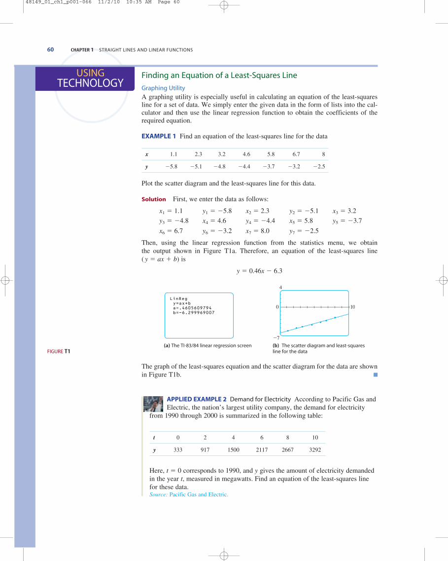
Finding an Equation of a Least-Squares Line
Graphing UtilityA graphing utility is especially useful in calculating an equation of the least-squaresline for a set of data. We simply enter the given data in the form of lists into the cal-culator and then use the linear regression function to obtain the coefficients of therequired equation.
EXAMPLE 1 Find an equation of the least-squares line for the data
x 1.1 2.3 3.2 4.6 5.8 6.7 8
y �5.8 �5.1 �4.8 �4.4 �3.7 �3.2 �2.5
Plot the scatter diagram and the least-squares line for this data.
Solution First, we enter the data as follows:
x1 � 1.1 y1 � �5.8 x2 � 2.3 y2 � �5.1 x3 � 3.2
y3 � �4.8 x4 � 4.6 y4 � �4.4 x5 � 5.8 y5 � �3.7
x6 � 6.7 y6 � �3.2 x7 � 8.0 y7 � �2.5
Then, using the linear regression function from the statistics menu, we obtain the output shown in Figure T1a. Therefore, an equation of the least-squares line ( y � ax � b) is
y � 0.46x � 6.3
(a) The TI-83/84 linear regression screen (b) The scatter diagram and least-squares line for the data
The graph of the least-squares equation and the scatter diagram for the data are shownin Figure T1b.
APPLIED EXAMPLE 2 Demand for Electricity According to Pacific Gas andElectric, the nation’s largest utility company, the demand for electricity
from 1990 through 2000 is summarized in the following table:
t 0 2 4 6 8 10
y 333 917 1500 2117 2667 3292
Here, t � 0 corresponds to 1990, and y gives the amount of electricity demandedin the year t, measured in megawatts. Find an equation of the least-squares linefor these data.Source: Pacific Gas and Electric.
100
_7
4
LinRegy=ax+ba=.4605609794b=-6.299969007
USINGTECHNOLOGY
FIGURE T1
60 CHAPTER 1 STRAIGHT LINES AND LINEAR FUNCTIONS
48149_01_ch1_p001-066 11/2/10 10:35 AM Page 60
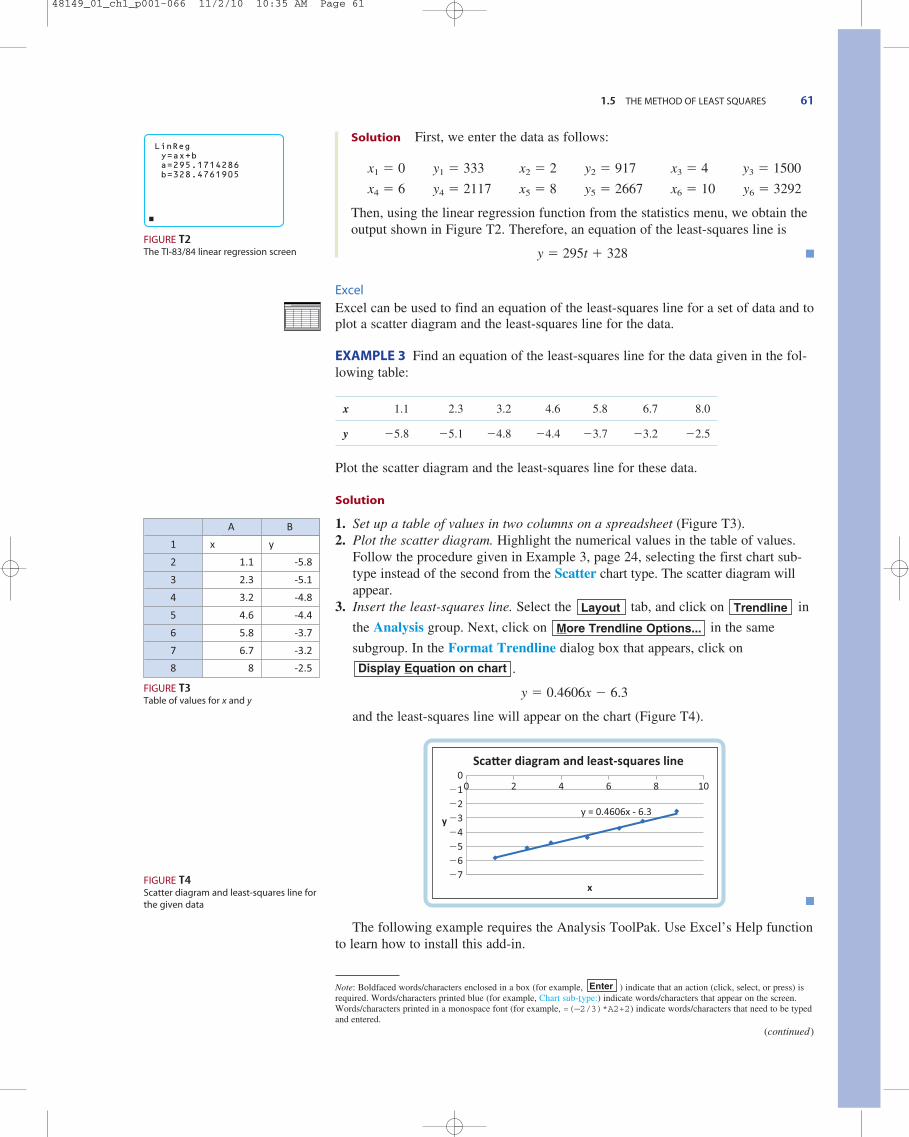
1.5 THE METHOD OF LEAST SQUARES 61
Solution First, we enter the data as follows:
x1 � 0 y1 � 333 x2 � 2 y2 � 917 x3 � 4 y3 � 1500
x4 � 6 y4 � 2117 x5 � 8 y5 � 2667 x6 � 10 y6 � 3292
Then, using the linear regression function from the statistics menu, we obtain theoutput shown in Figure T2. Therefore, an equation of the least-squares line is
y � 295t � 328
ExcelExcel can be used to find an equation of the least-squares line for a set of data and toplot a scatter diagram and the least-squares line for the data.
EXAMPLE 3 Find an equation of the least-squares line for the data given in the fol-lowing table:
x 1.1 2.3 3.2 4.6 5.8 6.7 8.0
y �5.8 �5.1 �4.8 �4.4 �3.7 �3.2 �2.5
Plot the scatter diagram and the least-squares line for these data.
Solution
1. Set up a table of values in two columns on a spreadsheet (Figure T3).2. Plot the scatter diagram. Highlight the numerical values in the table of values.
Follow the procedure given in Example 3, page 24, selecting the first chart sub-type instead of the second from the Scatter chart type. The scatter diagram willappear.
3. Insert the least-squares line. Select the tab, and click on in
the Analysis group. Next, click on in the same
subgroup. In the Format Trendline dialog box that appears, click on
.
y � 0.4606x � 6.3
and the least-squares line will appear on the chart (Figure T4).
The following example requires the Analysis ToolPak. Use Excel’s Help functionto learn how to install this add-in.
Sca�er diagram and least-squares line
�2�3�4�5�6
0�1
�7
0 42
x
y
6
y = 0.4606x - 6.3
8 10
Display Equation on chart
More Trendline Options...
TrendlineLayout
(continued)
Note: Boldfaced words/characters enclosed in a box (for example, ) indicate that an action (click, select, or press) isrequired. Words/characters printed blue (for example, Chart sub-type:) indicate words/characters that appear on the screen.Words/characters printed in a monospace font (for example, =(—2/3)*A2+2) indicate words/characters that need to be typedand entered.
Enter
x y
-5.82
1
-5.13
-4.84
-4.45
-3.76
-3.27
1.1
2.3
3.2
4.6
5.8
6.7
-2.58 8
A B
FIGURE T3Table of values for x and y
FIGURE T2The TI-83/84 linear regression screen
LinRegy=ax+ba=295.1714286b=328.4761905
FIGURE T4Scatter diagram and least-squares line forthe given data
48149_01_ch1_p001-066 11/2/10 10:35 AM Page 61

62 CHAPTER 1 STRAIGHT LINES AND LINEAR FUNCTIONS
APPLIED EXAMPLE 4 Demand for Electricity According to Pacific Gasand Electric, the nation’s largest utility company, the demand for
electricity from 1990 through 2000 is summarized in the following table:
t 0 2 4 6 8 10
y 333 917 1500 2117 2667 3292
Here, t � 0 corresponds to 1990, and y gives the amount of electricity in year t,measured in megawatts. Find an equation of the least-squares line for these data.
Solution
1. Set up a table of values on a spreadsheet (Figure T5).
2. Find the equation of the least-squares line for the data. Click on
in the Analysis group of the Data tab. In the Data Analysis
dialog box that appears, select , and then click . In the
Regression dialog box that appears, select the box, and
then enter the y-values by highlighting cells B2:B7. Next select the
box, and enter the x-values by highlighting cells A2:A7.
Click , and a SUMMARY OUTPUT worksheet will appear. In the third
table, you will see the entries shown in Figure T6. These entries give the value
of the y-intercept and the coefficient of x in the equation y � mx � b. In our
example, we are using the variable t instead of x, so the required equation is
y � 295t � 328
OK
Input X Range:
Input Y Range:
OK Regression
Data Analysis
328.4761905
295.1714286X Variable 1
Intercept
Coefficients
FIGURE T6Entries in the SUMMARY OUTPUT box
t y
3332
1
9173
15004
21175
26676
32927
0
2
4
6
8
10
A B
FIGURE T5Table of values for x and y
TECHNOLOGY EXERCISES
In Exercises 1–4, find an equation of the least-squares line for thegiven data.
1.
2.
3.
4.
5. MODELING WITH DATA According to Company Reports,Starbucks annual sales (in billions of dollars) for 2001through 2006 are as follows (x � 0 corresponds to 2001):
x �1.12 0.1 1.24 2.76 4.21 6.82
y 7.61 4.9 2.74 �0.47 �3.51 �8.94
x �2.1 �1.1 0.1 1.4 2.5 4.2 5.1
y 6.2 4.7 3.5 1.9 0.4 �1.4 �2.5
x 1.1 2.4 3.2 4.7 5.6 7.2
y �0.5 1.2 2.4 4.4 5.7 8.1
x 2.1 3.4 4.7 5.6 6.8 7.2
y 8.8 12.1 14.8 16.9 19.8 21.1 a. Find an equation of the least-squares line for these data.b. Use the result to estimate Starbucks sales for 2009,
assuming that the trend continued.Source: Company Reports.
6. MODELING WITH DATA The projected number of computers(in millions) connected to the Internet in Europe from 1998through 2002 is summarized in the following table (x � 0corresponds to the beginning of 1998):
a. Find an equation of the least-squares line for these data.b. Use the result of part (a) to estimate the projected number
of computers connected to the Internet in Europe at thebeginning of 2005, assuming that the trend continued.
Source: Dataquest, Inc.
Year, x 0 1 2 3 4
Net-ConnectedComputers, y 21.7 32.1 45.0 58.3 69.6
Year, x 0 1 2 3 4 5
Sales, y 2.65 3.29 4.08 5.29 6.37 7.79
48149_01_ch1_p001-066 11/2/10 10:35 AM Page 62

7. MODELING WITH DATA According to data from the Councilon Environmental Quality, the amount of waste (in mil-lions of tons per year) generated in the United States from1960 to 1990 was as follows:
(Let x be in units of 5 and let x � 1 represent 1960.)a. Find an equation of the least-squares line for these data. b. Use the result of part (a) to estimate the amount of waste
generated in the year 2000, assuming that the trend con-tinued.
Source: Council on Environmental Quality.
8. MODELING WITH DATA More and more travelers are pur-chasing their tickets online. According to industry projec-tions, the U.S. online travel revenue (in billions of dollars)from 2001 through 2005 is given in the following table (t � 0 corresponds to 2001):
a. Find an equation of the least-squares line for these data.b. Use the result of part (a) to estimate the U.S. online
travel revenue for 2006.Source: Forrester Research, Inc.
Year, t 0 1 2 3 4
Revenue, y 16.3 21.0 25.0 28.8 32.7
Year 1980 1985 1990
Amount, y 140 152 164
Year 1960 1965 1970 1975
Amount, y 81 100 120 124
SUMMARY OF PRINCIPAL FORMULAS AND TERMS 63
9. MODELING WITH DATA According to the U.S. Department ofEnergy, the consumption of energy by countries of theindustrialized world is projected to rise over the next 25 years. The consumption (in trillions of cubic feet) from2000 through 2025 is summarized in the following table:
(Let x be measured in 5-year intervals, and let x � 0 repre-sent 2000.)a. Find an equation of the least-squares line for these data. b. Use the result of part (a) to estimate the energy con-
sumption in the industrialized world in 2012.Source: U.S. Department of Energy.
10. MODELING WITH DATA With an aging population, thedemand for health care, as measured by outpatient visits, issteadily growing. The number of outpatient visits (in mil-lions) from 1991 through 2001 is recorded in the followingtable (x � 0 corresponds to 1991):
a. Find an equation of the least-squares line for these data.b. Use the result of part (a) to estimate the number of out-
patient visits in 2004, assuming that the trend continued.Source: PriceWaterhouse Coopers.
Year, x 0 1 2 3 4 5 6 7 8 9 10
Number ofVisits, y 320 340 362 380 416 440 444 470 495 520 530
Year 2000 2005 2010 2015 2020 2025
Consumption, y 214 225 240 255 270 285
Summary of Principal Formulas and TermsCHAPTER 1
1. Distance between two points
2. Equation of a circle 1x � h 22 � 1y � k 22 � r2
3. Slope of a nonvertical line
4. Equation of a vertical line x � a
5. Equation of a horizontal line y � b
6. Point-slope form of the equation y � y1 � m 1x � x1 2of a line
7. Slope-intercept form of the equation y � mx � bof a line
8. General equation of a line Ax � By � C � 0
m �y2 � y1
x2 � x1
d � 21x2 � x1 2 2 � 1 y2 � y1 2 2FORMULAS
48149_01_ch1_p001-066 11/2/10 10:35 AM Page 63

64 CHAPTER 1 STRAIGHT LINES AND LINEAR FUNCTIONS
TERMS
Cartesian coordinate system (2)
ordered pair (2)
coordinates (3)
parallel lines (12)
perpendicular lines (14)
function (28)
independent variable (28)
dependent variable (28)
domain (28)
range (28)
linear function (28)
total cost function (30)
revenue function (30)
profit function (30)
demand function (31)
supply function (32)
break-even point (41)
market equilibrium (43)
equilibrium quantity (43)
equilibrium price (43)
Concept Review QuestionsCHAPTER 1
Fill in the blanks.
1. A point in the plane can be represented uniquely by a/an_____ pair of numbers. The first number of the pair iscalled the _____, and the second number of the pair iscalled the _____.
2. a. The point P(a, 0) lies on the _____ axis, and the point P(0, b) lies on the _____ axis.
b. If the point P(a, b) lies in the fourth quadrant, then thepoint P(�a, b) lies in the _____ quadrant.
3. The distance between two points P(a, b) and P(c, d ) is_____.
4. An equation of a circle with center C(a, b) and radius r isgiven by _____.
5. a. If P1 1x1, y1 2 and P2 1x2, y2 2 are any two distinct points on a nonvertical line L, then the slope of L is m �_____.
b. The slope of a vertical line is _____.c. The slope of a horizontal line is _____.d. The slope of a line that slants upward is _____.
6. If L1 and L2 are distinct nonvertical lines with slopes m1
and m2, respectively, then: L1 is parallel to L2 if and only if_____; and L1 is perpendicular to L2 if and only if _____.
7. a. An equation of the line passing through the point P 1x1, y1 2 and having slope m is _____. It is called the_____ form of an equation of a line.
b. An equation of the line that has slope m and y-interceptb is _____. It is called the _____ form of an equation ofa line.
8. a. The general form of an equation of a line is _____.b. If a line has equation ax � by � c � 0 (b � 0), then its
slope is _____.
9. A linear function is a function of the form f (x) � _____.
10. a. A demand function expresses the relationship betweenthe unit _____ and the quantity _____ of a commodity.The graph of the demand function is called the _____curve.
b. A supply function expresses the relationship betweenthe unit _____ and the quantity _____ of a commodity.The graph of the supply function is called the _____curve.
11. If R(x) and C(x) denote the total revenue and the total costincurred in manufacturing x units of a commodity, then thesolution of the simultaneous equations y � C(x) and y �R(x) gives the _____ point.
12. The equilibrium quantity and the equilibrium price arefound by solving the system composed of the _____ equa-tion and the _____ equation.
In Exercises 1–4, find the distance between the two points.
1. (2, 1) and (6, 4) 2. (9, 6) and (6, 2)
3. (�2, �3) and (1, �7) 4. a 1
2, 13 b and a�
1
2, 213 b
In Exercises 5–10, find an equation of the line L that passesthrough the point (�2, 4) and satisfies the given condition.
5. L is a vertical line. 6. L is a horizontal line.
7. L passes through the point .a3, 7
2b
Review ExercisesCHAPTER 1
48149_01_ch1_p001-066 11/2/10 10:35 AM Page 64
REVIEW EXERCISES 65
8. The x-intercept of L is 3.
9. L is parallel to the line 5x � 2y � 6.
10. L is perpendicular to the line 4x � 3y � 6.
11. Find an equation of the line with slope � 12 and y-intercept
�3.
12. Find the slope and y-intercept of the line with equation 3x � 5y � 6.
13. Find an equation of the line passing through the point (2, 3)and parallel to the line with equation 3x � 4y � 8 � 0.
14. Find an equation of the line passing through the point (�1, 3) and parallel to the line joining the points (�3, 4)and (2, 1).
15. Find an equation of the line passing through the point (�2, �4) that is perpendicular to the line with equation 2 x � 3y � 24 � 0.
In Exercises 16 and 17, sketch the graph of the equation.
16. 3x � 4y � 24 17. �2x � 5y � 15
18. SALES OF MP3 PLAYERS Sales of a certain brand of MP3players are approximated by the relationship
S 1x 2 � 6000x � 30,000 10 � x � 5 2where S(x) denotes the number of MP3 players sold in yearx (x � 0 corresponds to the year 2007). Find the number ofMP3 players expected to be sold in 2012.
19. COMPANY SALES A company’s total sales (in millions ofdollars) are approximately linear as a function of time (inyears). Sales in 2006 were $2.4 million, whereas sales in2011 amounted to $7.4 million.a. Letting x � 0 correspond to 2006, find a function giv-
ing the company’s sales in terms of x.b. What were the sales in 2009?
20. Show that the triangle with vertices A(1, 1), B(5, 3), and C(4, 5) is a right triangle.
21. CLARK’S RULE Clark’s Rule is a method for calculating pedi-atric drug dosages based on a child’s weight. If a denotesthe adult dosage (in milligrams) and if w is the child’sweight (in pounds), then the child’s dosage is given by
a. Show that D is a linear function of w.b. If the adult dose of a substance is 500 mg, how much
should a 35-lb child receive?
22. LINEAR DEPRECIATION An office building worth $6 millionwhen it was completed in 2010 is being depreciated lin-early over 30 years with a scrap value of $0.a. What is the rate of depreciation?b. What will be the book value of the building in 2020?
D1w 2 �aw
150
23. LINEAR DEPRECIATION In 2006 a manufacturer installed anew machine in her factory at a cost of $300,000. Themachine is depreciated linearly over 12 years with a scrapvalue of $30,000.a. What is the rate of depreciation of the machine per year?b. Find an expression for the book value of the machine in
year t (0 � t � 12).
24. PROFIT FUNCTIONS A company has a fixed cost of $30,000and a production cost of $6 for each disposable camera itmanufactures. Each camera sells for $10.a. What is the cost function?b. What is the revenue function?c. What is the profit function?d. Compute the profit (loss) corresponding to production
levels of 6000, 8000, and 12,000 units, respectively.
25. DEMAND EQUATIONS There is no demand for a certain com-modity when the unit price is $200 or more, but the demandincreases by 200 units for each $10 decrease in price below$200. Find the demand equation and sketch its graph.
26. SUPPLY EQUATIONS Bicycle suppliers will make 200 bicyclesavailable in the market per month when the unit price is $50and 2000 bicycles available per month when the unit price is$100. Find the supply equation if it is known to be linear.
In Exercises 27 and 28, find the point of intersection of the lineswith the given equations.
27. 3x � 4y � �6 and 2x � 5y � �11
28.
29. BREAK-EVEN ANALYSIS The cost function and the revenuefunction for a certain firm are given by C(x) � 12x �20,000 and R(x) � 20x, respectively. Find the break-evenpoint for the company.
30. MARKET EQUILIBRIUM Given the demand equation 3x �p � 40 � 0 and the supply equation 2x � p � 10 � 0,where p is the unit price in dollars and x represents thequantity demanded in units of a thousand, determine theequilibrium quantity and the equilibrium price.
31. COLLEGE ADMISSIONS The accompanying data were com-piled by the Admissions Office of Carter College duringthe past 5 years. The data relate the number of collegebrochures and follow-up letters (x) sent to a preselected listof high school juniors who took the PSAT and the numberof completed applications (y) received from these students(both measured in thousands).
a. Derive an equation of the straight line L that passesthrough the points (2, 0.5) and (4, 1).
b. Use this equation to predict the number of completedapplications that might be expected if 6400 brochuresand follow-up letters are sent out during the next year.
Brochures Sent, x 1.8 2 3.2 4 4.8
Applications Completed, y 0.4 0.5 0.7 1 1.3
y �3
4 x � 6 and 3x � 2y � 3 � 0
48149_01_ch1_p001-066 11/2/10 10:35 AM Page 65

32. MARKET EQUILIBRIUM The demand equation for the Edmundcompact refrigerator is 2x � 7p � 1760 � 0, where x is thequantity demanded each week and p is the unit price in dollars. The supply equation for these refrigerators is 3x �56p � 2680 � 0, where x is the quantity the supplier willmake available in the market when the wholesale price is p dollars each. Find the equilibrium quantity and the equi-librium price for the Edmund compact refrigerators.
33. MODELING WITH DATA The average hourly salary (in dol-lars) of hospital nurses in metropolitan Boston from 2000through 2004 is given in the following table (x � 0 corre-sponds to 2000):
a. Find an equation of the least-squares line for these data.b. If the trend continued, what was the average hourly
salary of nurses in 2006?Source: American Association of Colleges of Nursing.
Year 2000 2001 2002 2003 2004
Hourly Salary, y 27 29 31 32 35
34. MODELING WITH DATA The Census Bureau projections offemale life expectancy at age 65 in the United States aresummarized in the following table (x � 0 corresponds to2000):
a. Find an equation of the least-squares line for these data.b. Use the result of part (a) to estimate the life expectancy
at 65 of a female in 2040. How does this result comparewith the given data for that year?
c. Use the result of part (a) to estimate the life expectancyat 65 of a female in 2030.
Source: U.S. Census Bureau.
Year, x 0 10 20 30 40 50
Years beyond 65, y 19.5 20.0 20.6 21.2 21.8 22.4
1. Plot the points A(�2, 1) and B(3, 4) on the same set ofaxes, and find the distance between A and B.
2. Find an equation of the line passing through the point (3, 1) and parallel to the line 3x � y � 4 � 0.
3. Let L be the line passing through the points (1, 2) and (3, 5). Is L perpendicular to the line 2x � 3y � 10?
4. The monthly total revenue function and total cost functionfor a company are R(x) � 18x and C(x) � 15x � 22,000,respectively, where x is the number of units produced andboth R(x) and C(x) are measured in dollars.
a. What is the unit cost for producing the product?b. What is the monthly fixed cost for the company?c. What is the selling price for each unit of the product?
5. Find the point of intersection of the lines 2x � 3y � �2and 9x � 12y � 25.
6. The annual sales of Best Furniture Store are expected to begiven by S1 � 4.2 � 0.4t million dollars t years from now,whereas the annual sales of Lowe’s Furniture Store areexpected to be given by S2 � 2.2 � 0.8t million dollars tyears from now. When will Lowe’s annual sales first sur-pass Best’s annual sales?
66 CHAPTER 1 STRAIGHT LINES AND LINEAR FUNCTIONS
The problem-solving skills that you learn in each chapter are building blocks for the rest of the course. Therefore, it is a good idea to makesure that you have mastered these skills before moving on to the next chapter. The Before Moving On exercises that follow are designed forthat purpose. After taking this test, you can see where your weaknesses, if any, are. Then you can log in at login.cengagebrain.com whereyou will find a link to CourseMate. Here, you can access additional Concept Quiz and Concept Review modules.
If you feel that you need additional help with these exercises, at this Website you can also use Tutorial Example Videos.
Before Moving On . . .CHAPTER 1
48149_01_ch1_p001-066 11/16/10 9:26 AM Page 66