1 lesson 8: basic monte carlo integration we begin the 2 nd phase of our course: study of general...

1

Lesson 8: Basic Monte Carlo integrationLesson 8: Basic Monte Carlo integration

• We begin the 2We begin the 2ndnd phase of our course: Study phase of our course: Study of general mathematics of MCof general mathematics of MC

• Consists of a progression:Consists of a progression:• Monte Carlo evaluation of integrals (4 ways)Monte Carlo evaluation of integrals (4 ways)• Basic numerical analysis framework (to explain the Basic numerical analysis framework (to explain the

4 ways)4 ways)• MC evaluation of integral equationsMC evaluation of integral equations• Generalization of this technique to solve general Generalization of this technique to solve general

differential equation setsdifferential equation sets

2

Monte Carlo Integration Monte Carlo Integration • Next set of mathematical tools: MC integration Next set of mathematical tools: MC integration • Our study so far of sampling from distributions has Our study so far of sampling from distributions has

provided us with the tools for MC simulationprovided us with the tools for MC simulation• MC integration will provide:MC integration will provide:

• More rigorous ideas of keeping scoreMore rigorous ideas of keeping score• Basic mathematical underpinnings of variance reduction. Basic mathematical underpinnings of variance reduction. • ““Abstract” approach to MC problem: ALMOST ALL MC Abstract” approach to MC problem: ALMOST ALL MC

PROBLEMS ARE INTEGRATIONSPROBLEMS ARE INTEGRATIONS

• Development of four particular methods using the Development of four particular methods using the framework. framework.

3

Four particular integration methodsFour particular integration methods

• We will now go over four particular variations We will now go over four particular variations on this theme: on this theme:

1.1. Rejection method Rejection method

2.2. Averaging method Averaging method

3.3. Control variates method Control variates method

4.4. Importance sampling method Importance sampling method

4

Rejection methodRejection method• This is a similar approach to the use of This is a similar approach to the use of

rejection methods in picking from a rejection methods in picking from a distribution. distribution.

• It is a "dart board" method in which we It is a "dart board" method in which we estimate the area under a functional curve by estimate the area under a functional curve by containing the curve in a rectangular "box", containing the curve in a rectangular "box", picking a point randomly in the box, and picking a point randomly in the box, and scoring 0 if it misses (i.e., is above the curve) scoring 0 if it misses (i.e., is above the curve) or the full rectangular area if it hits (i.e., is or the full rectangular area if it hits (i.e., is below the curve). below the curve).

• As before, we have to specify an upper bound As before, we have to specify an upper bound of the function, , and then proceed by: of the function, , and then proceed by: maxf

5

Rejection method (2)Rejection method (2)

1. Choose a value of uniformly between a and 1. Choose a value of uniformly between a and b. b.

2. Choose a value of uniformly between 0 and2. Choose a value of uniformly between 0 and

3. Score if 3. Score if

and score otherwise. and score otherwise.

ab

xx

1ˆˆ

x̂

f̂

maxf

xff ˆˆ abfI maxˆ

0ˆ I

6

Rejection method exampleRejection method example

Find using a rejection method. Find using a rejection method.

Answer: The maximum value of this function Answer: The maximum value of this function in the range is 4, so our procedure is:in the range is 4, so our procedure is:

1.1. Choose a value of uniformly between 0 and 2. Choose a value of uniformly between 0 and 2.


3.3. Score 8 if is less than ; otherwise score Score 8 if is less than ; otherwise score 0.0.

Find first two moments of this method and Find first two moments of this method and calculate the expected mean and SD of mean.calculate the expected mean and SD of mean.

2

0

2dxxI

x̂

f̂

f̂ 2x̂

7

Averaging methodAveraging method

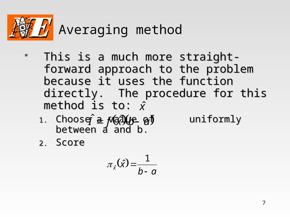
This is a much more straight-forward This is a much more straight-forward approach to the problem because it uses the approach to the problem because it uses the function directly. The procedure for this function directly. The procedure for this method is to: method is to:

1.1. Choose a value of uniformly between a and b. Choose a value of uniformly between a and b. 2.2. Score Score

x̂ abxfI ˆˆ

ab

xx

1ˆˆ

8

Averaging ExampleAveraging Example

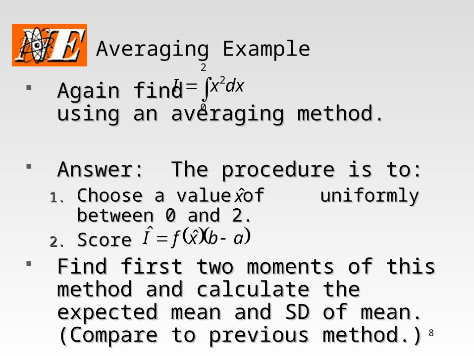
Again find using an Again find using an averaging method. averaging method.

Answer: The procedure is to:Answer: The procedure is to:1.1. Choose a value of uniformly between 0 Choose a value of uniformly between 0

and 2. and 2. 2.2. Score Score

Find first two moments of this method Find first two moments of this method and calculate the expected mean and and calculate the expected mean and SD of mean. (Compare to previous SD of mean. (Compare to previous method.)method.)

2

0

2dxxI

x̂

abxfI ˆˆ

9

Control variates methodControl variates method

This method is the first of two methods that This method is the first of two methods that utilize a user-supplied second function, , utilize a user-supplied second function, , which is chosen to be a "well behaved" which is chosen to be a "well behaved" approximation toapproximation to

What makes these methods so powerful is What makes these methods so powerful is that they allow the user to take use of a priori that they allow the user to take use of a priori knowledge about the function. knowledge about the function.

In the control variates method, the integral In the control variates method, the integral solution "begins" as the integral of the known solution "begins" as the integral of the known function:function:

and uses the Monte Carlo approach to find an and uses the Monte Carlo approach to find an

additive correction to this user-supplied guess. additive correction to this user-supplied guess.

b

a

h dxxhI

xh xf

10

Control variates method (2)Control variates method (2)

The procedure for this method is to: The procedure for this method is to: 1.1. Choose a value of uniformly between a and b. Choose a value of uniformly between a and b. 2.2. Score Score

Notice that there is NO variance introduced Notice that there is NO variance introduced through the part of the score.through the part of the score.

Obviously, then a good guess will result in a Obviously, then a good guess will result in a small difference and, therefore a small small difference and, therefore a small variance. variance.

• In the limit of a perfect guess, , there is In the limit of a perfect guess, , there is no correction and no therefore no variance. no correction and no therefore no variance.

• Not quite as obvious is the fact that if Not quite as obvious is the fact that if h(x)h(x) and and f(x)f(x) differ by a CONSTANT, we also have a 0 variance differ by a CONSTANT, we also have a 0 variance method.method.

hIabxhxfI ˆˆˆ

hI

xfxh

11

Control variates exampleControl variates example

Again find , this time using a Again find , this time using a control variates method withcontrol variates method with

Answer: Note the integral of Answer: Note the integral of h(x)h(x) over (0,2) is over (0,2) is 2. With this value known, the procedure is to: 2. With this value known, the procedure is to:


2.2. Score Score

Find first two moments of this method and Find first two moments of this method and calculate the expected mean and SD of mean. calculate the expected mean and SD of mean. (Compare to previous methods.)(Compare to previous methods.)

2

0

2dxxI

2

3xxh

22

ˆˆ2

32

x

x

12

Importance sampling methodImportance sampling method The final method is the importance The final method is the importance

sampling method. This technique is similar sampling method. This technique is similar to the control variates method, in that it to the control variates method, in that it takes advantage of a priori knowledge takes advantage of a priori knowledge about the function , but differs from it about the function , but differs from it in that its correction is in that its correction is multiplicativemultiplicative rather rather than additive. than additive.

The importance sampling method uses the The importance sampling method uses the approximate function as the probability approximate function as the probability distribution with which the variables are distribution with which the variables are drawn: drawn:

h

b

a

x I

xh

dxxh

xhx

ˆˆˆˆ

xf

xhx̂

13

Importance sampling (2)Importance sampling (2) The resulting score is:The resulting score is:

As with control variates, a "perfect" guess of As with control variates, a "perfect" guess of would result in a zero variance solution, would result in a zero variance solution, this time because, again, every score would this time because, again, every score would be exactly correct. be exactly correct.

(Note that, because of the normalization, a (Note that, because of the normalization, a guess equal to a MULTIPLE of guess equal to a MULTIPLE of f(x)f(x) will also will also work.)work.)

ˆˆˆ h

f xI I

h x

14

Importance sampling exampleImportance sampling example

Again find , this time using an Again find , this time using an importance sampling method withimportance sampling method with

• Answer: Since the integral of h(x) over the range (0,2) is 2, the resulting probability distribution from which to pick the x’s will be:

• Following the direct procedure for choosing from this distribution, we first determine the c.d.f, which is:

4

3

ˆ

xxx

2

0

2dxxI

2

3xxh

164

4

0

3 xxxP

x

15

Importance sampling exampleImportance sampling example

We then set this c.d.f. to the uniform deviate:

and invert to get the formula:

• Score is now:

• Find first two moments of this method and Find first two moments of this method and calculate the expected mean and SD of mean. calculate the expected mean and SD of mean. (Compare to previous methods.)(Compare to previous methods.)

xx

xfI

x ˆ4

ˆ

ˆˆˆ

42ˆ x

16

ˆ4x

16

2nd pass at integration: more rigor2nd pass at integration: more rigor• Theoretical underpinning is the Law of Large Theoretical underpinning is the Law of Large

NumbersNumbers• In one of our early lectures, we defined the In one of our early lectures, we defined the

mean of a continuous function as:mean of a continuous function as:

• And later worked out a Monte Carlo algorithm And later worked out a Monte Carlo algorithm with the same expectation:with the same expectation:

dxxxxb

a

xxN

xxx i

N

ii

usingchosen where,ˆ 1

17

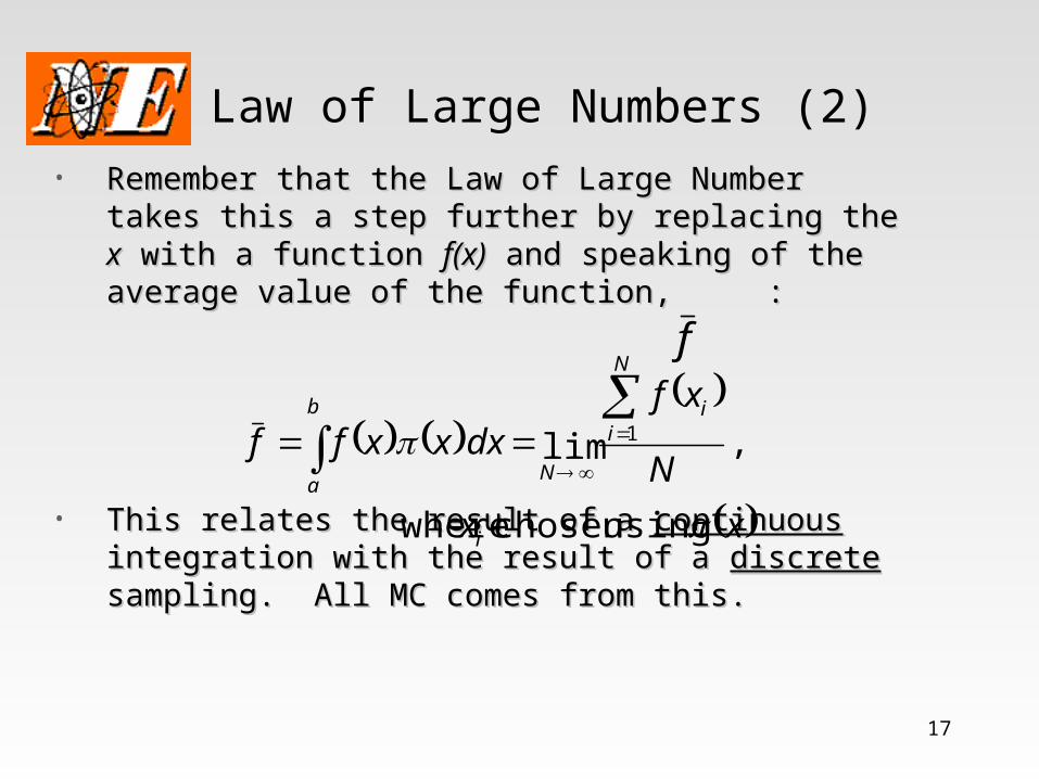
Law of Large Numbers (2)Law of Large Numbers (2)• Remember that the Law of Large Number takes this a Remember that the Law of Large Number takes this a

step further by replacing the step further by replacing the xx with a function with a function f(x)f(x) and and speaking of the average value of the function, :speaking of the average value of the function, :

• This relates the result of a This relates the result of a continuouscontinuous integration with integration with the result of a the result of a discretediscrete sampling. All MC comes from sampling. All MC comes from this.this.

f

xx

N

xfdxxxff

i

N

ii

N

b

a

usingchosen where

,lim 1

18

Using the Law of Large NumbersUsing the Law of Large Numbers• Putting our “goal” integration in this form requires Putting our “goal” integration in this form requires

that we multiply and divide by the probability that we multiply and divide by the probability distribution,distribution, (x)(x)

• Following the previous “rules” we have divided the Following the previous “rules” we have divided the integrand into two “pieces”: the score and the PDFintegrand into two “pieces”: the score and the PDF

• There is an implicit requirement that There is an implicit requirement that (x)>0(x)>0 for all for all xx for for which which f(x) is not 0 so that f(x)f(x) is not 0 so that f(x)(x)/(x)/(x) is defined(x) is defined

xx

N

xxf

dxxx

xfdxxfI

i

N

i i

i

N

b

a PDFscore

b

a

usingchosen where

,lim)( 1

""

19

Dirac notationDirac notation

• In our integrations so far, I have simplified In our integrations so far, I have simplified the mathematics a bit by always choosing x the mathematics a bit by always choosing x between a and b. between a and b.

xx

N

xxf

dxxx

xfdxxfI

i

N

i i

i

N

b

a PDFscore

b

a

usingchosen where

,lim)( 1

""

• I was careful to always choose x between a and b. I was careful to always choose x between a and b. What if I had not done this?What if I had not done this?

20

Dirac notation (2)Dirac notation (2)A more genearl way to approach this (which takes care of the A more genearl way to approach this (which takes care of the “domain question”) is to look at the Monte Carlo attack of the “domain question”) is to look at the Monte Carlo attack of the integral in TWO steps:integral in TWO steps:

(1) an approximation of (1) an approximation of f(x)f(x) itself using: itself using:

(2) a substitution of this functional approximation into the integral:(2) a substitution of this functional approximation into the integral:

( ) i

i i ii

f xf x x x w x x

x

1

1

( ) lim

lim

bN

i ibi a

Na

bN

i ii a

N

w x x dx

I f x dxN

w x x dx

N

21

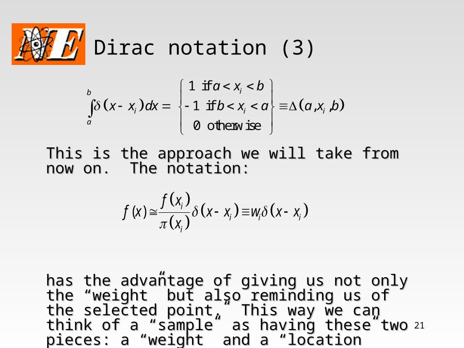
Dirac notation (3)Dirac notation (3)

1 if

1 if , ,

0 otherwise

ib

i i i

a

a x b

x x dx b x a a x b

This is the approach we will take from now on. The This is the approach we will take from now on. The notation:notation:

has the advantage of giving us not only the “weight” has the advantage of giving us not only the “weight” but also reminding us of the selected point. This way but also reminding us of the selected point. This way we can think of a “sample” as having these two we can think of a “sample” as having these two pieces: a “weight” and a “location”pieces: a “weight” and a “location”

( ) i

i i ii

f xf x x x w x x

x

22

Averaging methodAveraging method• The easiest of our four methods to put in this form The easiest of our four methods to put in this form

is the averaging method (which we previously is the averaging method (which we previously discussed second)discussed second)

• Recall that the procedure for this method is to: Recall that the procedure for this method is to: • Choose a value of uniformly between a and b. Choose a value of uniformly between a and b.

• Score Score

• In terms of our mathematical framework, this is In terms of our mathematical framework, this is equivalent to again using: equivalent to again using:

• and scoring with a direct use ofand scoring with a direct use of

ab

x

1

ˆ

abxfx

xfI ˆ

ˆ

ˆˆ

x̂

abxfI ˆˆ

23

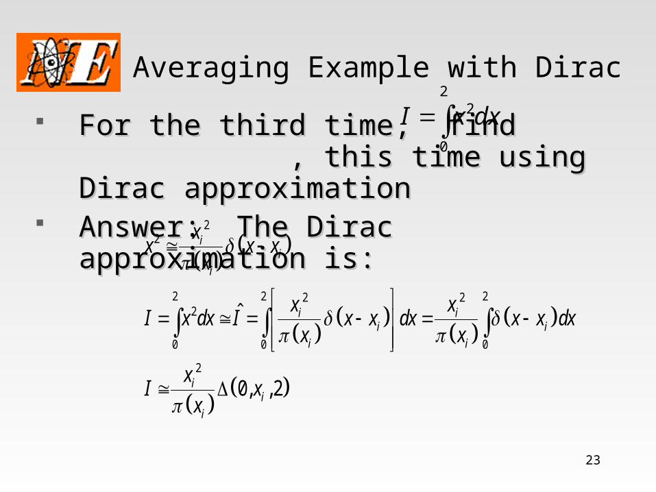
Averaging Example with DiracAveraging Example with Dirac

For the third time, find , this For the third time, find , this time using Dirac approximationtime using Dirac approximation

Answer: The Dirac approximation is:Answer: The Dirac approximation is:

2

0

2dxxI

22

2 2 22 22

0 0 0

2

ˆ

0, , 2

ii

i

i ii i

i i

ii

i

xx x x

x

x xI x dx I x x dx x x dx

x x

xI x

x

24

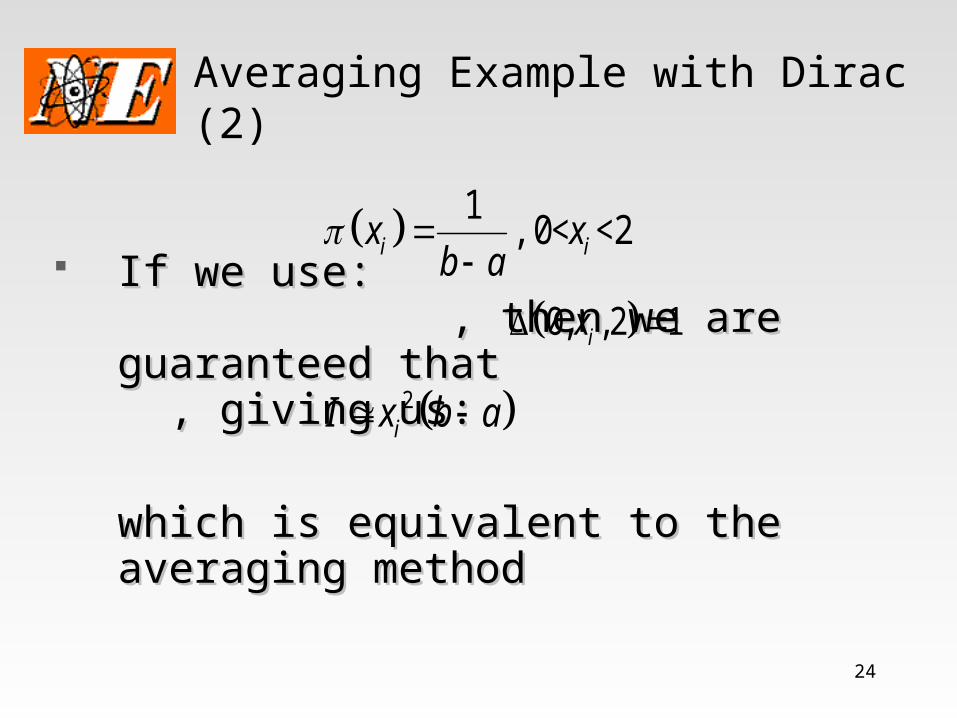
Averaging Example with Dirac (2)Averaging Example with Dirac (2)

If we use: , then we If we use: , then we are guaranteed that , giving are guaranteed that , giving us:us:

which is equivalent to the averaging which is equivalent to the averaging methodmethod

0, , 2 1ix

1, 0< <2i ix x

b a

2iI x b a

25

Averaging Example with Dirac (3)Averaging Example with Dirac (3)

If we use:If we use:

then plugging in gives us the importance then plugging in gives us the importance sampling result:sampling result:

or , 0< <2i

i i i ih

h xx h x x x

I

2

i ih h

i i

f x xI I I

h x h x

26

Rejection methodRejection method

Backing up to the rejection method, the procedure was:Backing up to the rejection method, the procedure was:1. Choose a value of uniformly between a and b. 1. Choose a value of uniformly between a and b.

2. Choose a value of uniformly between 0 and 2. Choose a value of uniformly between 0 and

3. Score if 3. Score if

and score otherwise. and score otherwise.

• In terms of our mathematical framework, this is In terms of our mathematical framework, this is equivalent to using: equivalent to using:

(for a uniform distribution between a and b) and …(for a uniform distribution between a and b) and …

ab

xx

1ˆˆ

x̂

f̂ maxf

xff ˆˆ abfI maxˆ

0ˆ I

27

Rejection method (2)Rejection method (2)

scoring with a scoring with a probability mixingprobability mixing strategy of: strategy of:

with probability with probability

or scoring or scoring

0 with probability 0 with probability

This mixed scoring strategy obviously has the This mixed scoring strategy obviously has the desired expected value ofdesired expected value of

xf

x ˆˆ

max

xxf

Ix ˆ

ˆ

ˆ

max

ˆ

f

xf

max

ˆ1

f

xf

28

Control variates methodControl variates method

The procedure for this method is to: The procedure for this method is to: 1.1. Choose a value of uniformly between a and b. Choose a value of uniformly between a and b. 2.2. Score Score

• where, where, h(x)h(x) is chosen as an easily integrated is chosen as an easily integrated approximation of approximation of f(x)+constantf(x)+constant

hIabxhxfI ˆˆˆ

x̂

29

Control variates method (2)Control variates method (2) In terms of our mathematical framework, this In terms of our mathematical framework, this

again uses a flat distribution and score with:again uses a flat distribution and score with:

h

h

b

a

b

a

Iabxhxf

xab

Ixhxf

x

dx

dxxh

xhxf

x

xhExhxfI

ˆˆ

ˆ

ˆˆ

ˆ

ˆˆ

ˆ

ˆˆˆˆ

30

Importance sampling methodImportance sampling method

The procedure for this method is to: The procedure for this method is to: 1.1. Choose a value of between a and b using a Choose a value of between a and b using a

probability distribution probability distribution h(x)h(x) that is “shaped like” that is “shaped like” f(x).f(x). 2.2. Score Score

In terms of our mathematical framework, this is a simple In terms of our mathematical framework, this is a simple replacement of the flat distribution of the averaging replacement of the flat distribution of the averaging method with the “better” distribution method with the “better” distribution h(x)h(x) (with allowance (with allowance for the fact that for the fact that h(x)h(x) is probably unnormalized): is probably unnormalized):

hIxh

xfI

ˆ

ˆˆ

x̂

31

Importance sampling method(2)Importance sampling method(2)

Giving us:Giving us:

h

N

i i

i

N

b

a

b

a

I

xhx

N

xxf

dxxx

xfdxxfI

where

,lim)( 1

,lim1

N

Ixhxf

I

N

ih

i

i

N

32

Solution of Integral EquationsSolution of Integral Equations

Application of our integration techniques to Application of our integration techniques to integral equationsintegral equations

• Introduction of Dirac notationIntroduction of Dirac notation• Conversion of differential equations to Conversion of differential equations to

integral equationsintegral equations• Solution of integral equationsSolution of integral equations• Solution of linked equationsSolution of linked equations

33

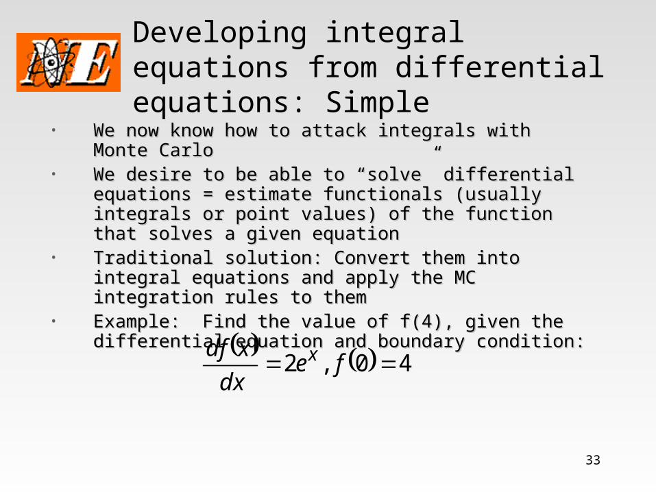
Developing integral equations from differential equations: SimpleDeveloping integral equations from differential equations: Simple

• We now know how to attack integrals with Monte CarloWe now know how to attack integrals with Monte Carlo• We desire to be able to “solve” differential equations = We desire to be able to “solve” differential equations =

estimate functionals (usually integrals or point values) of the estimate functionals (usually integrals or point values) of the function that solves a given equationfunction that solves a given equation

• Traditional solution: Convert them into integral equations and Traditional solution: Convert them into integral equations and apply the MC integration rules to themapply the MC integration rules to them

• Example: Find the value of f(4), given the differential Example: Find the value of f(4), given the differential equation and boundary condition:equation and boundary condition:

40,2 fedx

xdf x

34

Simple integral equations (2)Simple integral equations (2)

• Answer: We can integrate from 0 (the Answer: We can integrate from 0 (the known value) to the desired value to get:known value) to the desired value to get:

• Now we apply one of the four integration Now we apply one of the four integration methods to the integral in the equation:methods to the integral in the equation:

duedu

du

udf u 4

0

4

0

2 dueff u4

0

204

duef u4

0

244

35


4

41 0

0

1 1

4 4 2 4 2lim

4 2 0, ,4 lim lim

iuu

i u ii

N

u iiu

N

N N

u i ii i

N N

ee u u w u u

u

w u u du

f e duN

w u w

N N

• NOTE: From now on, I will skip the summation and NOTE: From now on, I will skip the summation and division by N and just write the formula for ONE division by N and just write the formula for ONE sample:sample:

24 4 2 0, ,4 4 0, ,4

iu

i u i ii

ef w w u u

u

36


The normal procedure for this method is to: The normal procedure for this method is to: 1.1. Choose a value of between a and b using a Choose a value of between a and b using a

probability distribution probability distribution (x)(x) (of YOUR choosing). (of YOUR choosing). 2.2. Score Score

So, let’s do it.So, let’s do it. What PDF should we use?What PDF should we use?

Lazy man’s PDF: uniformLazy man’s PDF: uniform Optimum PDF: ? (You tell me…)Optimum PDF: ? (You tell me…)

ˆ2

4 4ˆ

x

i

ef

x

w

x̂

37

Linked equationsLinked equations

• When you are faced with linked equation sets, When you are faced with linked equation sets, the principles are the same, put you have to be the principles are the same, put you have to be more careful:more careful:

• Putting in multiple boundary conditionsPutting in multiple boundary conditions• Keeping up with multiple sampled variables (each Keeping up with multiple sampled variables (each

equation will have one)equation will have one)• Most tricky: Realizing and adapting to CHANGING Most tricky: Realizing and adapting to CHANGING

LIMITS on the integrals (after the first)LIMITS on the integrals (after the first)• MUCH more difficult to optimize the choice of the MUCH more difficult to optimize the choice of the

PDFs usedPDFs used

38

Linked equation exampleLinked equation example• Example: Find Example: Find f(2)f(2) for the second order differential for the second order differential

equation:equation:

• In order to make it fit the category, we will start be re-In order to make it fit the category, we will start be re-writing as the linked set:writing as the linked set:

20,10 ,42

2

ffxdx

xfd

10 ,

20,4

fxgdx

xdf

gxdx

xdg

39

Linked equation example (2)Linked equation example (2)

• Applying our tools to the second equation first, we begin Applying our tools to the second equation first, we begin by transforming it into an integral equation for the value by transforming it into an integral equation for the value at x=2:at x=2:

• Using our MC integration approximation, we get:Using our MC integration approximation, we get:

• How do we get the ? Answer: We estimate it from How do we get the ? Answer: We estimate it from the other equation.the other equation.

2

0

12 dxxgf

ˆˆ2 1 where 0 2

ˆ f

g xf w x

x

xg ˆ

40


• Applying our tools to the first equation first, we begin by Applying our tools to the first equation first, we begin by transforming it into an integral equation for the value attransforming it into an integral equation for the value at

::

• The resulting procedure is:The resulting procedure is:1.1. Choose a value of usingChoose a value of using

2.2. Choose a value of usingChoose a value of using

3.3. Score:Score:

ˆ 4

4

0

ˆˆ ˆ ˆ2 2 where 0

ˆ

x

g

ug x u du w u x

u

4ˆ2

ˆ2 1 =1

ˆ ˆg

f

uwu

f wx x

4,0ˆx

xx ˆ

xx ˆˆ xu ˆ,0ˆ uu ˆˆ

41


• Now let’s do it.Now let’s do it.• What PDF’s to use?What PDF’s to use?

• FlatFlat• Better than flatBetter than flat

42

HWHW

43

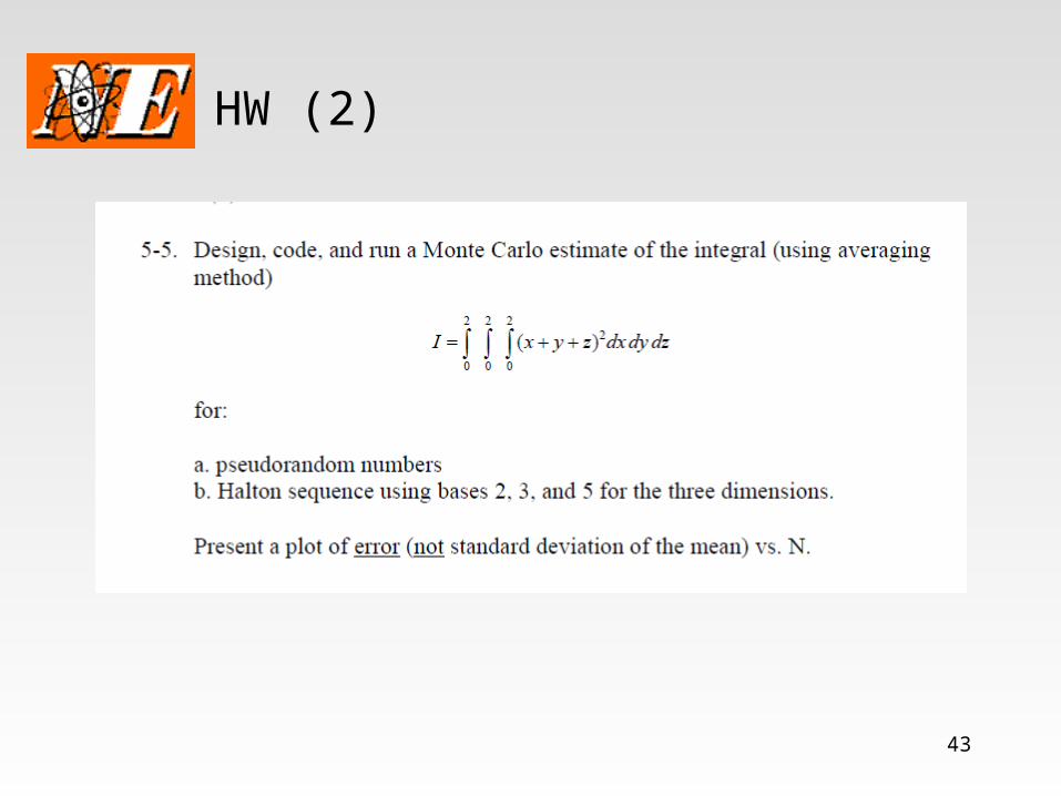
HW (2)HW (2)

1 lesson 8: basic monte carlo integration we begin the 2 nd phase of our course: study of general...

Documents