1 lecture on wireless measurements & modeling prof. maria papadopouli university of crete...
Post on 22-Dec-2015
213 views
TRANSCRIPT

1
Lecture on Wireless Measurements & Modeling
Prof. Maria PapadopouliUniversity of Crete
ICS-FORTHhttp://www.ics.forth.gr/mobile

Agenda
• Introduction on Mobile Computing & Wireless Networks• Wireless Networks - Physical Layer• IEEE 802.11 MAC• Wireless Network Measurements & Modeling • Location Sensing• Performance of VoIP over wireless networks• Mobile Peer-to-Peer computing
2

Empirical measurements• Can be beneficial in revealing
– deficiencies of a wireless technology – different phenomena of the wireless access & workload
• Impel modelling efforts to produce more realistic models & synthetic traces
• Enable meaningful performance analysis studies using such empirical, synthetic traces and models
Highlight the ability of empirical-based models to capture the characteristics of the user-workload and provide a flexible framework for using them in performance analysis
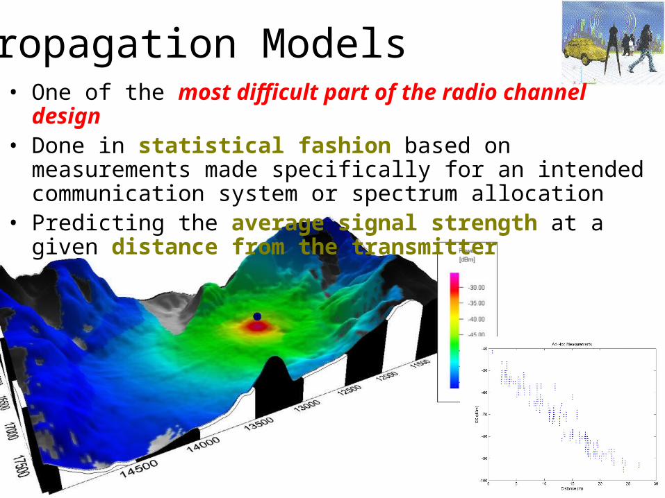
Propagation Models• One of the most difficult part of the radio channel design• Done in statistical fashion based on measurements made specifically
for an intended communication system or spectrum allocation• Predicting the average signal strength at a given distance from the
transmitter
4

Signal Power Decay with Distance
• A signal traveling from one node to another experiences fast (multipath) fading, shadowing & path loss
• Ideally, averaging RSS over sufficiently long time interval excludes the effects of multipath fading & shadowing general path-loss model:
P(d) = P0 – 10n log10 (d/do)
n: path loss exponent P(d): the average received power in dB at distance d P0 is the received power in dB at a short distance d0
5
_
_

7
Monitoring
• Depending on type of conditions that need to be measured, monitoring needs to be performed at
• Certain layers • Spatio-temporal granularities
• Monitoring tools – Are not without flaws – Several issues arise when they are used in parallel for
thousands devices of different types & manufacturers:• Fine-grain data sampling• Time synchronization• Incomplete information• Data consistency

8
Monitoring & Data Collection
• Fine spatio-temporal detail monitoring can Improve the accuracy of the performance estimates but also Increase the energy spendings and detection delay
Network interfaces may need to • Monitor the channel in finer & longer time scales• Exchange this information with other devices

9
Challenges in Monitoring (1/2)
• Identification of the dominant parameters through – sensitivity analysis studies
• Strategic placement of monitors at – Routers– APs, clients, and other devices
• Automation of the monitoring process to reduce human intervention in managing the
• Monitors • Collecting data

10
Challenges in Monitoring (2/2)
• Aggregation of data collected from distributed monitors to improve the accuracy while maintaining low overhead in terms of
• Communication • Energy
• Cross-layer measurements, collected data spanning from the physical layer up to the application layer, are required
11
Wireless Networks
– Are extremely complex – Have been used for many different purposes– Have their own distinct characteristics due to radio
propagation characteristics & mobility e.g., wireless channels can be highly asymmetric and time varying
Note: Interaction of different layers & technologies creates many situations
that cannot be foreseen during design & testing stages of technology development

12
Empirically-based Measurements
• Real-life measurement studies can be particularly beneficial in revealing– deficiencies of a wireless technology – different phenomena of the wireless access and the workload
• Rich sets of data can – Impel modeling efforts to produce more realistic models– Enable more meaningful performance analysis studies

13
Unrealistic Assumptions
– Models & analysis of wired networks are valid for wireless networks
– Wireless links are symmetric– Link conditions are static– The density of devices in an area is uniform– The communication pairs are fixed – Users move based on random-walk models

14
Wireless Access Parameters
• Traffic workload– In different time-scales– In different spatial scales (e.g., AP, client, infrastructure)– In bytes, number of packets, number of flows, application-mix
• Delays – Jitter and delay per flow– Statistics at an AP and/or channel
• User mobility patterns• Link conditions• Network topology

15
Traffic Load Analysis
• As the wireless user population increases, the characterization of traffic workload can facilitate
• More efficient network management • Better utilization of users’ scarce resources
• Application-based traffic characterization

16
Hourly Session arrival rates
17
Traffic Load at APs
• Wide range of workloads that log-normality is prevalent
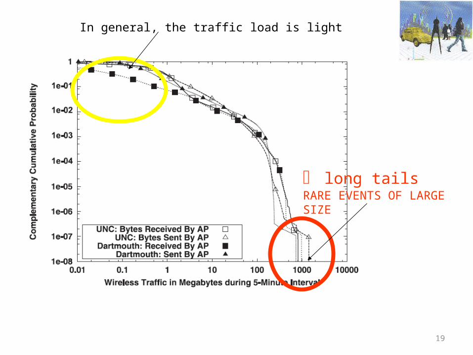
• In general, traffic load is light, despite the long tails
• No clear dependency with type of building the AP is located exists– Although some stochastic ordering is present in
• Tail of the distributions
• Dichotomy among APs is prominent in both infrastructures:
APs dominated by uploaders APs dominated by downloaders
• As the total received traffic at an AP ↑– There is also ↑ in its total traffic sent – ↓ in the sent-to-received ratio

18
Traffic load at APs
• Substantial number of non-unicast packets• Number of unicast received packets strongly correlated with
number of unicast sent packets (in log-log scale)• Most of APs send & receive packets of relatively small size• Significant number of APs show rather asymmetric packet sizes
– APs with large sent & small receive packets– APs with small sent & large receive packets
• Distributions of the number of associations & roaming operations are heavy-tailed
• Correlation between the traffic load & number of associations in log-log scale
19
In general, the traffic load is light
long tailsRARE EVENTS OF LARGESIZE

20
Wide-range of workloads
As total received traffic at an AP ↑ its total traffic sent ↑
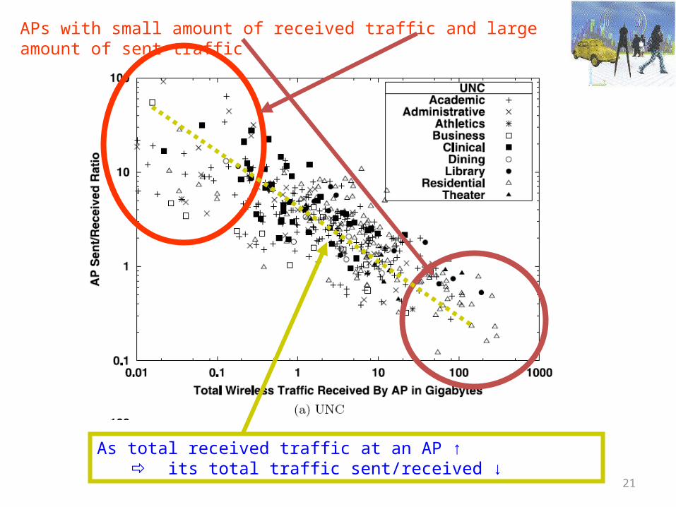
21
APs with small amount of received traffic and large amount of sent traffic
As total received traffic at an AP ↑ its total traffic sent/received ↓

22
The number of unicast received packets strongly correlated with the number of unicast sent packets (in log-log scale)

23
Asymmetry in the sizes of sent & received packets at an AP
Majority of APs with small sent and received packet sizes

24
Correlation between traffic load & # of associations

25
Application-based Traffic Characterization
Using port numbers to classify flows may lead to significant amounts of misclassified traffic due to:– Dynamic port usage– Overlapping port ranges– Traffic masquerading
• Often peer-to-peer & streaming applications:– Use dynamic ports to communicate– Port ranges of different applications may overlap– May try to masquerade their traffic under well-known “non-
suspicious” ports, such as port 80

26
Desirable Properties for Models
– Accuracy– Tractability– Scalability– Reusability– “Easy” interpretation

Related work• Rich literature in traffic characterization in wired networks
– Willinger, Taqqu, Leland, Park on self-similarity of Ethernet LAN traffic– Crovela, Barford on Web traffic– Feldmann, Paxson on TCP– Paxson, Floyd on WAN– Jeffay, Hernandez-Campos, Smith on HTTP
• Traffic generators for wired traffic– Hernandez-Campos, Vahdat, Barford, Ammar, Pescape, …
• P2P traffic– Saroiu, Sen, Gummadi, He, Leibowitz, …
• On-line games– Pescape, Zander, Lang, Chen, …
• Modelling of wireless traffic– Meng et al.

Dimensions in Modeling Wireless Access
• Intended user demand• User mobility patterns
– Arrival at APs– Roaming across APs
• Channel conditions• Network topology
Mobility models
• Group or individual mobility• Spontaneous or controlled• Pedestrian or vehicular• Known a priori or dynamic
• Random-walk based models– Randway model in ns-2
• Markov-based model

A Very Simple Channel Model
Idle BusyPii
Pbb
Pbi
Pib
• A channel can be in the idle or busy state• Markov-based model allows us to determine:
• How much time the system spends in each state• Probability of being in a particular state
In real rife, there is non-stationarity due dynamic phenomena
Compute stationary probabilities
Gilbert model
Main approaches for traffic generation
• Packet-level replay– An exact reproduction of a collected trace in terms of packet
arrival times, size, source, destination, content type Reflects specific traffic conditions
– Suffers from arbitrary delays e.g., interrupts, service mechanisms, scheduling processes difficult to incorporate feedback-loop characteristics
• Source-level generation Allows the underlying network, protocol, & application layer to
specify & control the packet arrival process– Simplest example: infinite source model

Our approach
Inspired by the source-level (or network independent) modelling
Assumptions:1. Client arrivals at an infrastructure (initiated by humans) at a large extent are not affected by the underlying network technology
2. Very low % of packet loss at the network layer flow arrivals & sizes approximate intended user traffic demand

1 2 3 0Session
Wired Network
Wireless Network
Router
Internet
User A
User B
AP 1 AP 2
AP3Switch
disconnection
Flow
time
Events
Arrivals
t1 t2 t3 t7t6t5t4

Traffic Demand Parameters
• Session– arrival process– starting AP
• Flow within session– arrival process– number of flows– size (in bytes)
Captures interaction between clients & network
Above packet-level analysis
Wireless infrastructure & acquisition
• 26,000 students, 3,000 faculty, 9,000 staff in over 729-acre campus• 488 APs (April 2005), 741 APs (April 2006)• SNMP data collected every 5 minutes• Several months of SNMP & SYSLOG data from all APs• Packet-header traces:
– Two weeks (in April 2005 and April 2006)– Captured on the link between UNC & rest of Internet via a high-
precision monitoring card

Related modeling approaches
Flow-level modeling by Meng [mobicom ‘04] No session concept Weibull for flow interarrivals Lognormal for flow sizes AP-level over hourly intervals
Hierarchical modeling by Papadopouli [wicon ‘06] Time-varying Poisson process for session arrivals
BiPareto for in-session flow numbers & flow sizes Lognormal for in-session flow interarrivals
Sessions capture the non-stationarity of traffic workload

Modeling methodology
1. Selection of models (e.g., various distributions)2. Fitting parameters using empirical traces3. Evaluation and comparison of models• Visual inspection e.g., CCDFs & QQ plots of models vs. empirical data• Statistical-based criteria e.g., QQ/simulation envelopes, Kullback-Liebler divergence• Systems-based criteria e.g., throughput, delay, jitter, queue size
4. Validation of models5. Generalization of models

Synthetic trace generation

Synthetic traces based on empirical ones
Generate session arrivals within each session: generate number of flows for each flow: generate flow arrivals & sizes based on specific models
• Session arrivals: using hourly, building-specific empirical traces• Flow-related data: using empirical traces of different spatial scales
original data from the real-life infrastructureProduced by this process:
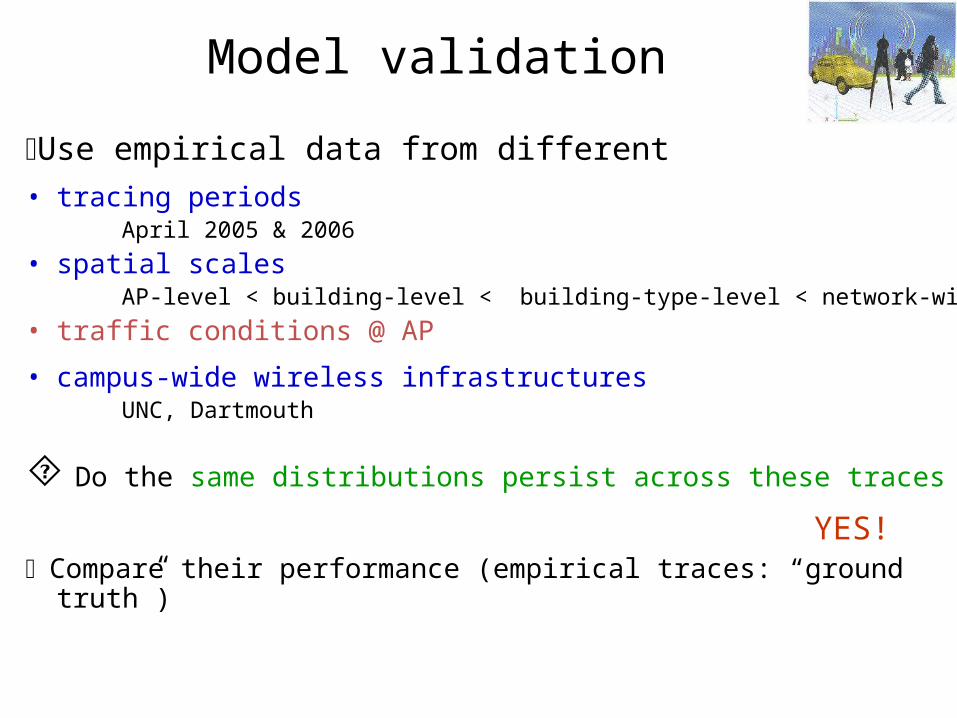
Model validation
Use empirical data from different• tracing periods
April 2005 & 2006• spatial scales
AP-level < building-level < building-type-level < network-wide• traffic conditions @ AP
• campus-wide wireless infrastructures UNC, Dartmouth
Do the same distributions persist across these traces ?
Compare their performance (empirical traces: “ground truth”)
YES!

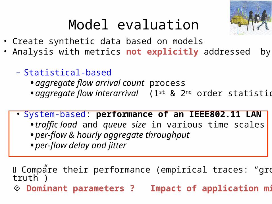
Model evaluation• Create synthetic data based on models• Analysis with metrics not explicitly addressed by the models
– Statistical-based• aggregate flow arrival count process• aggregate flow interarrival (1st & 2nd order statistics)
• System-based: performance of an IEEE802.11 LAN• traffic load and queue size in various time scales• per-flow & hourly aggregate throughput• per-flow delay and jitter
Compare their performance (empirical traces: “ground truth”)

Modeling in Various Spatio-temporal Scales
Sufficient spatial detail Scalable Amenable to analysis
Hourly period @ AP
Network-wide
ObjectiveScales
Tradeoff with respect to accuracy, scalability & reusability

Scalability vs. Accuracy: Flow Interarrivals
EMPIRICAL
BDLG(DAY)
BDLGTYPE(DAY)NETWORK(TRACE)
Spatial /Temporal Scales

Scalability vs. Accuracy: Number of Flow Arrivals in an Hour
EMPIRICAL
BDLG(DAY)
NETWORK(TRACE)
BDLGTYPE(TRACE)
Model evaluation• Create synthetic data based on models• Analysis with metrics not explicitly addressed by the models
– Statistical-based• aggregate flow arrival count process• aggregate flow interarrival (1st & 2nd order statistics)
• System-based: performance of an IEEE802.11 LAN• traffic load and queue size in various time scales• per-flow & hourly aggregate throughput• per-flow delay and jitter
Compare their performance (empirical traces: “ground truth”) Dominant parameters ? Impact of application mix?

Wireless Networks
RouterInternet
User A AP
AP
Switch
User B
Scenario
User C
Varioustraffic, channelconditions
Network monitor
Collected traces
StatisticalAnalysis
TestbedDeploymen
t
Monitoring &Data collection
CertainProtocol
Evaluationat AP
Iterative process
Networkmonitor
Select testbed Protocol evaluation Cross validation
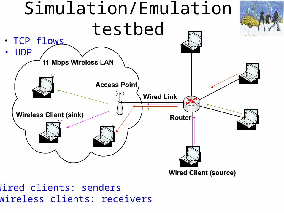
Simulation/Emulation testbed• TCP flows• UDP
• Wired clients: senders• Wireless clients: receivers
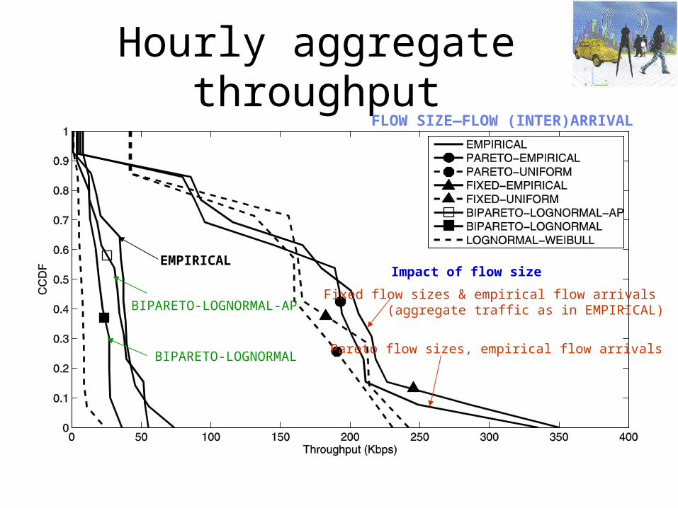
Hourly aggregate throughput
EMPIRICAL
BIPARETO-LOGNORMAL
Fixed flow sizes & empirical flow arrivals (aggregate traffic as in EMPIRICAL)
Pareto flow sizes, empirical flow arrivals
FLOW SIZE—FLOW (INTER)ARRIVAL
BIPARETO-LOGNORMAL-AP
Impact of flow size

Per-flow throughput
EMPIRICALBIPARETO-LOGNORMAL-AP
BIPARETO-LOGNORMAL
Fixed flow sizes & empirical number of flows
FLOWSIZE—FLOWARRIVAL
Pareto flow sizes & uniform flow arrivals
Pareto flow sizesdue to large % of small size flows (= MSS)

Impact of application mix on per-flow throughput
AP with 85% web traffic
AP with 50% web & 40% p2p traffic
AP with 80% p2p traffic
TCP-based scenario

UDP traffic scenario Wireless hotspot AP Wireless clients downloading Wired traffic transmit at 25Kbps Total aggregate traffic sent in CBR & in empirical is the same
Empirical: 1.4 KbpsBipareto-Lognormal-AP: 2.4 KbpsBipareto-Lognormal: 2.6 Kbps
Large differences in the distributions

ConclusionsModel validation
over two different periods (2005 and 2006)
over two different campus-wide infrastructures (UNC & Dartmouth)BiPareto captures well the flow sizes
over heavy & normal traffic conditions @ AP
using statistical-based metrics
using system-based metrics hourly aggregate throughput per-flow delay per-flow throughput

Conclusions (con’t)
Accuracy:
• our models perform very close to the empirical traces
• popular models deviate substantially from the empirical traces
Scalability:
• same distributions at various spatial & temporal scales• group of APs per bldg addresses scalability-accuracy tradeoffs
Accurate and scalable models of wireless demand
Conclusions (con’t)
Application mix of AP traffic mostly web: very accurate models both web & p2p : models are ok mostly p2p: large deviations from empirical data
Modelling P2P traffic is challenging due to the increased number, diversity, complexity & unpredictability in user interaction
Both flow size and flow interarrivals
Impact of various parameters

Revisiting modelling approach• Physical meaning of the models and their parameters• Client profile
– e.g., depending on the application-mix, amount of traffic • Group mobility• Multiple network interfaces• Cooperative client models• Dependencies among traffic demand & network conditions
– Impact of underlying network conditions on application & usage patterns

UNC/FORTH web archive
Online repository of models, tools, and traces– Packet header, SNMP, SYSLOG, synthetic traces, …http://netserver.ics.forth.gr/datatraces/ Free login/ password to access it
Simulation & emulation testbeds that replay synthetic traces for various traffic conditions
Mobile Computing Group @ University of Crete/FORTH http://www.ics.forth.gr/mobile/
57
Application-based traffic characterization
• Most popular applications: web browsing and peer-to-peer (81% of the total traffic). Most users are also dominated by these two applications.
• Network management & scanning: responsible for 17% of the total flows.• While building-aggregated traffic application usage patterns appear similar, the application cross-section
varies within APs of the same building.• Most wireless clients appear to use the wireless network for one specific application that dominates
their traffic share.• File transfer flows (e.g., ftp and peer-to-peer) are heavier in the wired network than in the wireless one.• There is a dichotomy among APs, in terms of their dominant application type and downloading and
uploading behavior.