1 lecture notes
TRANSCRIPT
1
Lecture Notes
Applied Mathematics for Business, Economics, and the Social Sciences (4th Edition);
by Frank S. Budnick

2
Chapter 2: Linear Equations
Definition: Linear equations are first degree equations. Each variable in the equation is raised to the first power.
Definition: A linear equation involving two variables x and y has the standard form
ax + by= c where a, b and c are constants and a and b cannot both equal zero.
Note: The presence of terms having power other than 1 or
product of variables, e.g. (xy) would exclude an equation from
being linear. Name of the variables may be different from x and
y.
Examples:
1. 3𝑥 + 4𝑦 = 7 is linear equation, where 𝑎 = 3, 𝑏 = 4, 𝑐 = 7
2. √𝑥 = 5 + 𝑦 is non-liner equation as power of 𝑥 is not 1. Solution set of an equation Given a linear equation ax + by= c, the solution set for the equation (2.1) is the set of all ordered pairs (x, y) which satisfy the equation.
𝑆 = {(𝑥, 𝑦)|𝑎𝑥 + 𝑏𝑦 = 𝑐} For any linear equation, S consists of an infinite number of elements. Method
1. Assume a value of one variable

3
2. Substitute this into the equation 3. Solve for the other variable
Example
Given 2𝑥 + 4𝑦 = 16 , determine the pair of values which satisfy the equation when x=-2 Solution: Put x=-2 in given equation gives us 4y=16-4, i.e y=3. So the pair (-2,3) is a pair of values satisfying the given equation. Linear equation with n variables Definition A linear equation involving n variables x1, x2, . . . , xn has the general form
a1 x1 + a2 x2+ . . . + an xn = b
where 𝑎 , 𝑎 , ⋯ , 𝑎 are non-zero. Definition: The solution set S of a linear equation with n variables as
defined above is the collection of n-tuples (𝑥 , 𝑥 , ⋯ , 𝑥 ) such
that 𝑆 = {(𝑥 ,⋯ , 𝑥 )| 𝑎 𝑥 + ⋯+ 𝑎 𝑥 = 𝑏}.
As in the case of two variables, there are infinitely many values in the solution set. Example
Given an equation 4𝑥 − 2𝑥 + 6𝑥 = 0, what values satisfy
the equation when 𝑥 = 2 and 𝑥 = 1.

4
Solution: Put the given values of 𝑥 and 𝑥 in the above
equation gives 𝑥 = 7. Thus (2,7,1) is a solution of the above
equation.
Graphing two variable equations A linear equation involving two variables graphs as a straight line in two dimensions. Method:
1. Set one variable equal to zero 2. Solve for the value of other variable 3. Set second variable equal to zero 4. Solve for the value of first variable 5. The ordered pairs (0, y) and (x, 0) lie on the line 6. Connect these points and extend the line in both
directions. Example
Graph the linear equation 2𝑥 + 4𝑦 = 16
Solution: In lectures
x-intercept The x-intercept of an equation is the point where the graph of the equation crosses the x-axis, i.e. y=0. y-intercept The y-intercept of an equation is the point where the graph of the equation crosses the y-axis, i.e. x=0 Note: Equations of the form x=k has no y-intercept and equations of the form y=k has no x-intercept

5
Slope Any straight line with the exception of vertical lines can be
characterized by its slope. Slope represents the inclination of a
line or equivalently it shows the rate at which the line raises
and fall or how steep the line is.
Explanation: The slope of a line may be positive, negative, zero or undefined. The line with slope
1. Positive then the line rises from left to right 2. Negative then the line falls from left to right 3. Zero then the line is horizontal line 4. Undefined if the line is vertical line
Note: The sign of the slope represents whether the line falling or raising. Its magnitude shows the steepness of the line. Two point formula (slope) Given any two point which lie on a (non-vertical) straight line, the slope can be computed as the ratio of change in the value of y to the change in the value of x.
Slope = =
Δ𝑦 = change in the value of y
Δ𝑥 = change in the vale of x Two point formula (mathematically) The slope m of a straight line connecting two points (x1, y 1) and (x 2, y 2) is given by the formula

6
Slope= 2− 1
2− 1
Example
Compute the slope of the line segment connecting the two
points (−2, 3) and (1, −9).
Solution: Here we have (𝑥 , 𝑦 ) = (−2,3) and (𝑥 , 𝑦 ) = (1,−9)
so using the above formula we get
Slope=− −
−(− )= −4
Note: Along any straight line the slope is constant. The line connecting any two points will have the same slope. Slope Intercept form Consider the general form of two variable equation as
𝑎𝑥 + 𝑏𝑦 = 𝑐 We can write it as
𝑦 = −𝑎
𝑏𝑥 +
𝑐
𝑎
The above equation is called the slope-intercept form. Generally, it is written as:
𝑦 = 𝑚𝑥 + 𝑘 𝑚 = slope, 𝑘 = y-intercept Example Rewrite the equation
−𝑥 + 2𝑦
4= 3𝑥 − 𝑦
and find the slope and 𝑦 -intercept.

7
Solution: Rewriting the above we get 𝑦 =
𝑥 + 0. Thus slope
is
and y-intercept is zero.
Determining the equation of a straight line Slope and Intercept
This is the easiest situation to find an equation of line, if slope
of a line is -5 and y-intercept is (0, 15) then we have
m= -5, k = 15. We can write down
𝑦 = −5𝑥 + 15
as an equation of line, i.e. 5𝑥 + 𝑦 = 15.
Slope and one point
If we are given the slope of a line and some point that lies on
the line, we can substitute the know slope m and coordinates of
the given point into 𝑦 = 𝑚𝑥 + 𝑘 and solve for 𝑘.
Given a non-vertical straight line with slope m and containing the point (x1, y1), the slope of the line connecting (x1, y1) with any other point (x, y) is given by
𝑚 =𝑦 − 𝑦
𝑥 − 𝑥
Rearranging gives: 𝑦 − 𝑦 = 𝑚(𝑥 − 𝑥 )
Example

8
Find the equation of line having slope m = −2 and passing
through the point (2, 8).
Solution: Here (𝑥 , 𝑦 ) = (2,8) and 𝑚 = −2, so putting the
values in the above equation yields
𝑦 − 8 = −2(𝑥 − 2) 2𝑥 + 𝑦 = 12.
Parallel and perpendicular lines Two lines are parallel if they have the same slope, i.e.
𝑚 = 𝑚 .
Two lines are perpendicular if their slopes are equal to the
negative reciprocal of each other, i.e. 𝑚 𝑚 = −1. Example
Find an equation of line through the point (2, −4) and parallel to
the line 8𝑥 − 4𝑦 = 20.
Solution: From the given equation we have 𝑦 = 2𝑥 − 5. Let
𝑚 = 2 is the slope of the line. Then slope of the required line
is same, i.e. 𝑚 = 2. Thus required equation of line is
𝑦 − (−4) = 2(𝑥 − 2)
2𝑥 − 𝑦 = 8.

9
Lecture 2,3
Chapter 3:Systems of Linear Equations Definition A System of Equations is a set consisting of more than one equation. Dimension: One way to characterize a system of equations is by its dimensions. If system of equations has ‘m’ equations and ‘n’ variables, then the system is called an “m by n system”. In other
words, it has 𝑚 × 𝑛 dimensions. In solving systems of equations, we are interested in identifying values of the variables that satisfy all equations in the system simultaneously. Definition The solution set for a system of linear equations may be a Null
set, a finite set or an infinite set. Methods to find the solutions set 1. Graphical analysis method 2. Elimination method 3. Gaussian elimination method Graphical Analysis (2 x 2 system) We discuss three possible outcomes of the solution of 2 x 2 system. 1. Unique solution:
We draw the two lines and If two lines intersect at only one
point, say (𝑥 , 𝑦 ), then the coordinates of intersection point
(𝑥 , 𝑦 ), represent the solution for the system of equations. The system is said to have a unique solution.

10
2. No solution:
If two lines are parallel (recall that parallel lines have same slope but different y-intercept) then such a system has no solution. The equations in such a system are called inconsistent. 3. Infinitely many solutions:
If both equations graph on the same line, an infinite number of points are common in two lines. Such a system is said to have infinitely many solutions.
Graphical analysis by slope-Intercept relationships Given a (2 × 2) system of linear equations (in slope-intercept
form)
𝑦 = 𝑚 𝑥 + 𝑘
𝑦 = 𝑚 𝑥 + 𝑘
where 𝑚 and 𝑚 represent the two slopes and 𝑘 and 𝑘 denote the two y-intercepts then it has
I. Unique solution if 𝑚 𝑚 .
II. No Solution if 𝑚 = 𝑚 but 𝑘 𝑘 .
III. Infinitely many solutions if 𝑚 = 𝑚 and 𝑘 = 𝑘 .
Graphical solutions Limitations:
I. Good for two variable system of equations II. Not good for non-integer values
III. Algebraic solution is preferred The Elimination Procedure (2 x 2 system)

11
Given a (2 × 2) system of equations I. Eliminate one of the variable by multiplying or adding the
two equations II. Solve the remaining equation in terms of remaining variable
III. Substitute back into one of the given equation to find the value of the eliminated variable
Example Solve the system of equations
2𝑥 + 4𝑦 = 20
3𝑥 + 𝑦 = 10 Solution: Page 90 in Book or in Lectures Example
Solve the system of equations
3𝑥 − 2𝑦 = 6
−15𝑥 + 10𝑦 = −30 Solution: Page 91 in Book/in Lectures
Gaussian Elimination Method
This method can be used to solve systems of any size. The method begins with the original system of equations. Using row operations, it transforms the original system into an equivalent system from which the solution may be obtained easily. Recall that an equivalent system is one which has the same solution as the original system. In contrast to the Elimination procedure, the
transformed system maintain 𝑚 × 𝑛 dimension Basic Row Operations 1. Both sides of an equation may be multiplied by a nonzero
constant. 2. Equations or non-zero multiples of equations may be added or

12
subtracted to another equation. 3. The order of equations may be interchanged. Example Determine the solution set for the given system of equations, using Gaussian elimination method.
3𝑥 − 2𝑦 = 7
2𝑥 + 4𝑦 = 10 Solution: In Lectures
(m × 2) systems, m >2 When there are more than two equations involving only two variables then
1. We solve two equations first to get a point (𝑥, 𝑦) 2. Put the values in the rest of the equations 3. If all equations are satisfied then system has unique solution
(𝑥, 𝑦). 4. If we get no solution at (1) then system has no solution. 5. If there are infinitely many solutions at step (1), then we select
two different equations and repeat (1). Example
Determine the solution set for the given (4 × 2) system of equations,
𝑥 + 2𝑦 = 8
2𝑥 − 3𝑦 = −5
−5𝑥 + 6𝑦 = 8
𝑥 + 𝑦 = 7
Solution: In Lectures or on Page 94 in reference book.
Gaussian elimination procedure for 3 x 3 system

13
The procedure of Gaussian elimination method for the 3 x 3 system is same as for 2 x 2 system. First we will form coefficient transformation for 3 x 3 system, then convert it to transformed system.
Example1 Determine the solution set for the following system of equations
5𝑥 − 4𝑥 + 6𝑥 = 24
3𝑥 − 3𝑥 + 𝑥 = 54
−2𝑥 + 𝑥 − 5𝑥 = 30
Solution: The coefficient matrix of the above system is
[5 −4 6 243 −3 1 54
−2 1 −5 30]
Applying the row operations 3 − 5 , 2 + 5 , + , we get
the following form of the above system.
[5 −4 6 240 3 13 −1980 0 0 0
]
As one whole row is equal to zero, hence the system of equations
has infinitely many solutions.
Example2 Determine the solution set for the following system of equations
𝑥 − 𝑥 + 𝑥 = −5
3𝑥 + 𝑥 − 𝑥 = 25
2𝑥 + 𝑥 + 3𝑥 = 20
Solution: The coefficient matrix of the above system is
[1 −1 1 −53 1 −1 252 1 3 20
]

14
Applying the row operations 3 − ,
, 2 − , −
, 3 − , 4 − , −
,
, we get the following form of
the above system,
[1 0 0 50 1 0 100 0 1 0
].
Thus we have a unique solution 𝑥 = 5, 𝑥 = 10, 𝑥 = 0.
Example3 Determine the solution set for the following system of equations
−2𝑥 + 𝑥 + 3𝑥 = 10
10𝑥 − 5𝑥 − 15𝑥 = 30
𝑥 + 𝑥 − 3𝑥 = 25
Solution: The coefficient matrix of the above system is
[−2 1 3 1010 −5 −15 301 1 −3 25
]
Applying the row operations 5 + , + 2 ,
, −
, −
, we get the following form of the above system.
[1 0 −2 50 0 0 600 1 −1 20
]
From row 2 we get 0 = 60, hence the above system of linear
equations has no solution.
Application

15
Product mix problem: A variety of applications are concerned
with determining the quantitates of different products which satisfy
specific requirements
Example
A company produces three products. Each needs to be
processed through 3 different departments, with following data.
Department Products
1 2 3
Hours
available/week
A 2 2.5 3 1200
B 3 2.5 2 1150
C 4 3 2 1400
Determine whether there are any combination of three products
which would exhaust the weekly capacities of the three
departments?
Solution: Let 𝑥 , 𝑥 , 𝑥 be the number of units produced per
week of product 1, 2 and 3. The conditions to be specified are
expressed by the following system of equations.
2𝑥 + 3.5𝑥 + 3𝑥 = 1200 (Department A)
3𝑥 + 2.5𝑥 + 2𝑥 = 1150 (Department B)
4𝑥 + 3𝑥 + 2𝑥 = 1400 (Department C)

16
Now solving the above system by Gaussian elimination method
we will get 𝑥 = 200, 𝑥 = 100 and 𝑥 = 150.

17
Lecture 04,05
Chapter 4: Mathematical Functions Definition: A function is a mathematical rule that assigns to each input value one and only one output value.
Definition: The domain of a function is the set consisting of all possible input values.
Definition: The range of a function is the set of all possible output values. Notation The assigning of output values to corresponding input values is often called as mapping. The notation
𝑓(𝑥) = 𝑦
represents the mapping of the set of input values of 𝑥 into the
set of output values 𝑦, using the mapping rule 𝑓.
The equation
𝑦 = 𝑓(𝑥) denotes a functional relationship between the variables 𝑥 and
𝑦. Here 𝑥 means the input variable and 𝑦 means the output
variable, i.e. the value of 𝑦 depends upon and uniquely
determined by the values of 𝑥.
The input variable is called the independent variable and the output variable is called the dependent variable. Some examples
1. The fare of taxi depends upon the distance and the day of the week.
2. The fee structure depends upon the program and the type of education (on campus/off campus) you are admitting in.

18
3. The house prices depend on the location of the house.
Note: The variable 𝑥 is not always the independent variable, 𝑦 is
not always the dependent variable and 𝑓 is not always the rule
relating 𝑥 and 𝑦. Once the notation of function is clear then, from the given notation, we can easily identify the input variable, output
variable and the rule relating them, for example 𝑢 = 𝑔(𝑣) has
input variable 𝑣, output variable 𝑢 and 𝑔 is the rule relating 𝑢 and
𝑣. Example (Weekly Salary Function) A person gets a job as a salesperson and his salary depends upon the number of units he sells each week. Then, dependency of weekly salary on the units sold per week can be represented as
𝑦 = 𝑓(𝑥), where 𝑓 is the name of the salary function. Suppose your employer has given you the following equation for
determining your weekly salary: 𝑦 = 100 𝑥 + 5000
Given any value of x will result in the value of y with respect to the
function f. If x = 5, then y = 5500. We write this as, y = f(5) =5500. Example Given the functional relationship
f(x) = 5x − 10, Find f(0), f(−2) and f(a + b).
Solution: As 𝑓(𝑥) = 5𝑥 − 10, so
𝑓(0) = 5(0) − 10 = −10
𝑓(−2) = 5(−2) − 10 = −20
𝑓(𝑎 + 𝑏) = 5𝑎 + 5𝑏 − 10.

19
Domain and Range Recall that the set of all possible input values is called the domain of a function. Domain consists of all real values of the independent variable for which the dependent variable is defined and real. Example
Determine the domain of the function 𝑓(𝑥) =
− 2.
Solution: 𝑓(𝑥) is undefined at 4 − 𝑥 = 0, which gives that give
function is not defined at 𝑥 = ±2. Thus
Domain(f) = {𝑥|𝑥 𝑎 𝑎𝑛 𝑥 ±2}
Restricted domain and range
Up to now we have solved mathematically to find the domains of some types of functions. But for some real world problems, there may be more restriction on the domain e.g. in the weekly salary equation:
𝑦 = 100 𝑥 + 5000 Clearly, the number of units sold per week can not be negative. Also, they can not be in fractions, so the domain in this case will
be all positive natural numbers {1,2,3, … }. Further, the employer can also put the condition on the maximum number of units sold per week. In this case, the domain will be defined as:
D = {1,2, … , u} where u is the maximum number of units sold. Multivariate Functions
For many mathematical functions, the value of the dependent variable depends upon more than one independent variable.

20
Definition: A functions which contain more than one independent variable are called multivariate function.
Definition: A function having two independent variables is called bivariate function.
They are denoted by 𝑧 = 𝑓(𝑥, 𝑦), where 𝑥 and 𝑦 are the
independent variables and 𝑧 is the dependent variable e.g.
𝑧 = 2𝑥 + 5𝑦. In general the notation for a function 𝑓 where the value of
dependent variable depends on the values of 𝑛 independent
variables is 𝑧 = 𝑓(𝑥 ,⋯ , 𝑥 ). For example,
𝑧 = 2𝑥 + 5𝑥 + 4𝑥 − 4𝑥 + 𝑥 .
Types of Functions Constant Functions A constant function has the general form
𝑦 = 𝑓(𝑥) = 𝑎 Here, domain is the set of all real numbers and range is the single
value 𝑎 , e.g. 𝑓(𝑥) = 20. Linear Functions A linear function has the general (slope-intercept) form
𝑦 = 𝑓(𝑥) = 𝑎 𝑥 + 𝑎
where 𝑎 is slope and 𝑎 is 𝑦-intercept. For example 𝑦 = 2𝑥 + 3
is represented by a straight line with slope 2 and y-intercept 3.

21
The weekly salary function is also an example of linear function. Quadratic Function
A quadratic function has the general form 𝑦 = 𝑓(𝑥) = 𝑎 𝑥
+ 𝑎 𝑥 + 𝑎
provided that 𝑎 0, e.g. 𝑦 = 2𝑥 + 3. Cubic Function
A cubic function has the general form
𝑦 = 𝑓(𝑥) = 𝑎 𝑥 + 𝑎 𝑥
+ 𝑎 𝑥 + 𝑎
provided that 𝑎 0, e.g. 𝑦 = 𝑓(𝑥) = 𝑥 − 50𝑥 + 10𝑥 − 1. Polynomial Functions
A polynomial function of degree 𝑛 has the general form
𝑦 = 𝑓(𝑥) = 𝑎 𝑥 + ⋯+ 𝑎 𝑥 + 𝑎
Where 𝑎 , ⋯ , 𝑎 and 𝑎 are real constants such that 𝑎 0. All the previous types of functions are polynomial functions. Rational Functions A rational function has the general form
𝑦 = 𝑓(𝑥) =𝑔(𝑥)
(𝑥)
Where 𝑔(𝑥) and (𝑥) are both polynomial functions, e.g.
22
𝑦 = 𝑓(𝑥) =2𝑥
5𝑥 − 2𝑥 + 3.
Composite functions A composite function exists when one function can be viewed as
a function of the values of another function. If 𝑦 = 𝑔(𝑢) and
𝑢 = (𝑥) then composite function
𝑦 = 𝑓(𝑥) = 𝑔( (𝑥)).
Here 𝑥 must be in the domain of and (𝑥) must be in the
domain of 𝑔. For example, if 𝑦 = 𝑔(𝑢) = 3𝑢 + 4𝑢 and 𝑢 = (𝑥) =
𝑥 + 8, then 𝑔( (−2)) = 132.
Graphical Representation of Functions
The function of one or two variables (independent) can be represented graphically. The functions of one independent variable are graphed in two dimensions, 2-space. The functions in two independent variables are graphed in three dimension, 3-space.
Method of graphing 1) To graph a mathematical function, one can simply assign
different values from the domain of the independent variable and compute the values of dependent variable.
2) Locate the resulting order pairs on the co-ordinate axes, the
vertical axis (𝑦-axis) is used to denote the dependent variable
and the horizontal axis (𝑥-axis) is used to denote the independent variable.
3) Connect all the points approximately. Vertical Line Test By definition of a function, to each element in the domain there
23
should correspond only one element in the range. This allows a simple graphical check to determine whether a graph represents a function or not. If a vertical line is drawn through any value in the domain, it will intersect the graph of the function at one point only. If the vertical line intersects at more than one point then, the graph depicts a relation and not a function.

24
Lecture 05,06
Chapter 5:Linear functions, Applications
Recall that a linear function f involving one independent variable x
and a dependent variable y has the general form
𝑦 = 𝑓(𝑥) = 𝑎 𝑥 + 𝑎 ,
where 𝑎 0 and 𝑎 are constants. Example Consider the weekly salary function
𝑦 = 𝑓(𝑥) = 300𝑥 + 2500 where y is defined as the weekly salary and x is the number of units sold per week.
Clearly, this is a weekly function in one independent variable 𝑥. 1. 2500 represents the base salary, i.e. when no units are sold per
week and 300 is the commission of each unit sold. 2. The change in weekly salary is directly proportional to the
change in the no. of units sold. 3. Slope of 3 indicates the increase in weekly salary associated
with each additional unit sold.
In general, a linear function having the form 𝑦 = 𝑓(𝑥) = 𝑎 𝑥 + 𝑎
a change in the value of 𝑦 is directly proportional to a change in
the variable 𝑥. Linear function in two independent variables
A linear function f involving two independent variables x and x_2
and a dependent variable y has the general form
y = f(x , x ) = a x + a x + a
where a and a are non-zero constants and a is any constant.
1. This equation tells us that the variable 𝑦 depends jointly on the
values of 𝑥 and 𝑥 .

25
2. The value of 𝑦 is directly proportional to the changes in the
values of 𝑥 and 𝑥 . Example Assume that a salesperson salary depends on the number of units sold of each of two products, i.e. the salary function is given as
y = 300x + 500 x + 2500 where 𝑦 = weekly salary, 𝑥 is number of units sold of product 1
and 𝑥 is number of units sold of product 2. This salary function gives a base salary of 2500, commission of 300 on each unit sold of product 1 and 500 on each unit sold of product 2. Linear cost function
The organizations are concerned with the costs as they reflect the money flowing out of the organisation. The total cost usually consists of two components: total variable cost and total fixed cost. These two components determine the total cost of the organisation. Example A firm which produces a single product is interested in
determining the functions that expresses annual total cost 𝑦 as a
function of the number of units produced 𝑥. Accountants indicate
that the fixed expenditure each year are 50,000. They also have
estimated that raw material costs for each unit produced are 5.50,
labour costs per unit are 1.50 in the assembly department, 0.75 in
the finishing room, and 1.25 in the packaging and shipping
department. Find the total cost function.

26
Solution Total cost function = total variable cost + total fixed cost
Total fixed cost = 50,000 Total variable cost = total raw material cost + total labour cost
𝑦 = 𝑓(𝑥) = 5.5 𝑥 + (1.5 𝑥 + 0.75𝑥 + 1.25𝑥) + 50,000
= 9𝑥 + 50,000.
The 9 represents the combined variable cost per unit of $9. That
is, for each additional unit produced, total cost will increase by $9.
Linear Revenue function Revenue: The money which flows out into an organisation from
either selling or providing services is often referred to as revenue.
Total Revenue = Price × Quantity sold
Suppose a firm sells product. Let and x be the price of the
product and number of units per product respectively. Then the
revenue = x + ⋯+ x .
Linear Profit function
Profit: The profit of an organisation is the difference between total
revenue and total cost. In equation form if total revenue is
denoted by (x) and Total cost is (x), where x is quantity
produced and sold, then profit (x) is defined as
𝑃(𝑥) = (𝑥) − 𝐶(𝑥). 1. If total revenue exceeds total cost the profit is positive 2. In such case, profit is referred as net gain or net profit 3. On the other hand the negative profit is referred to as a net loss
or net deficit.

27
Example A firm sells single product for $65 per unit. Variable costs per unit are $20 for materials and $27.5 for labour. Annual fixed costs are
$100,000. Construct the profit function stated in terms of 𝑥, which is the number of units produced and sold. How much profit is earned if annual sales are 20,000 units.
Solution: Here (𝑥) = 65𝑥 and total annual cost is made up for
material costs, labour costs, and fixed cost.
𝐶(𝑥) = 20𝑥 + 27.5 𝑥 + 100,000 = 47.5 𝑥 + 100,000.
Thus
𝑃(𝑥) = (𝑥) − 𝐶(𝑥) = 17.5𝑥 − 100,000.
As 𝑥 = 20,000, so 𝑃(20,000) = 250,000.
Straight Line Depreciation When organizations purchase an item, usually cost is allocated for the item over the period the item is used. Example A company purchases a vehicle costing $20,000 having a useful life of 5 years, then accountants might allocate $4,000 per year as a cost of owning the vehicle. The cost allocated to any given period is called depreciation. The value of the truck at the limp of purchase is $20,000 but, after 1 year the price will be $20000- $4000 = $ 16000 and so forth. In this case, depreciation can also be thought of as an amount by which the book value of an asset has decreased over the period of time.
Thus, the book value declines as a linear function over time. If 𝑉

28
equals the book value of an asset and t equals time (in years) measured from the purchase date for the previously
mentioned truck, then V = f(t). Linear demand function A demand function is a mathematical relationship expressing the way in which the quantity demanded of an item varies with the price charged for it. The relationship between these two variables, quantity demanded and price per unit, is usually inversely proportional, i.e. a decrease in price results in increase in demand. Most demand functions are nonlinear, but there are situations in which the demand relationship either is, or can be approximated by a linear function.
𝑢𝑎𝑛 𝑦 𝑚𝑎𝑛 = = 𝑓( 𝑐 𝑢𝑛 )
Linear Supply Function A supply function relates market price to the quantities that suppliers are willing to produce or sell. The supply function implicates that what is brought to the market depends upon the price people are willing to pay. In contrast to the demand function, the quantity which suppliers are willing to supply usually varies directly with the market price. The higher the market price, the more a supplier would like to produce and sell. The lower the price, the less a supplier would like to produce and sell.
𝑢𝑎𝑛 𝑦 𝑢 = = 𝑓(𝑚𝑎 𝑘 𝑐 )
Break-Even Models Break-even model is a set of planning tools which can be useful in managing organizations. One significant indication of the

29
performance of a company is reflected by how much profit is earned. Break-even analysis focuses upon the profitability of a firm and identifies the level of operation or level of output that would result in a zero profit. The level of operations or output is called the break-even point. The break-even point represents the level of operation at which total revenue equals total cost. Any changes from the level of operations will result in either a profit or a loss. Break-even analysis is mostly used when:
1. Firms are offering new products or services. 2. Evaluating the pros and cons of starting a new business.
Assumption Total cost function and total revenue function are linear. Break-even Analysis
In break-even analysis the main goal is to determine the break-even point.
The break-even point may be expressed in terms of i. Volume of output (or level of activity) ii. Total sale in dollars iii. Percentage of production capacity e.g. a firm will break-even at 1000 units of output, when total
sales equal 2 million dollars or when the firm is operating 60% of its plant capacity.
Method of performing break-even analysis
1. Formulate total cost as a function of 𝑥 , the level of output.
2. Formulate total revenue as a function of 𝑥. 3. As break-even conditions exist when total revenue equals
total cost, so we set 𝐶(𝑥) equals (𝑥) and solve for 𝑥. The
resulting value of 𝑥 is the break-even level of output and

30
denoted by 𝑥 .
An alternate, to step 3 is to construct the profit function 𝑃(𝑥) = (𝑥) − 𝐶(𝑥), set 𝑃(𝑥) equal to zero and solve to find 𝑥 .
Example A Group of engineers is interested in forming a company to produce smoke detectors. They have developed a design and estimated that variable costs per unit, including materials, labor, and marketing costs are $22.50. Fixed costs associated with the formation, operation, management of the company and purchase of the machinery costs $250,000. They estimated that the selling price will be 30 dollars per detector.
a) Determine the number of smoke detectors which must be sold in order for the firm to break-even on the venture.
b) Preliminary marketing data indicate that the firm can expect to sell approximately 30,000 smoke detectors over the life of the project, if the detectors are sold at $30 per unit. Determine expected profits at this level of output.
Solution:
a) If 𝑥 equals the number of smoke detectors produced and
sold, the total revenue function (𝑥) = 30𝑥. The total cost
function is 𝐶(𝑥) = 22.5 𝑥 + 250,000. We put (𝑥) = 𝐶(𝑥) to
get 𝑥 = 33333.3 units.
b) 𝑃(𝑥) = (𝑥) − 𝐶(𝑥) = 7.5 𝑥 − 250,000. Now at 𝑥 = 30,000,
we have 𝑃(30,000) = −25,000. Thus the expected loss is
$25,000.
Market Equilibrium Given supply and demand functions of a product, market equilibrium exits if there is a price at which the quantity demanded equals the quantity supplied.

31
Example
Suppose demand and supply functions have been estimated for
two competing products.
1= 100 − 2 + 3 (Demand, Product 1)
2= 150 + 4 − (Demand, Product 2)
1= 2 − 4(Supply, Product 1)
2= 3 − 6(Supply, Product 2)
Determine the price for which the market equilibrium would
exist.
Solution: The demand and supply functions are linear. The
quantity demanded of a given product depends on the price of the
product and also on the price of the competing product and the
quantity supplied of a product depends only on the price of that
product.
Market equilibrium would exist in this two-product market place if
prices existed and were offered such that 1= 1
and 2= 2
,
solving we get = 221 and = 260. Putting the values in above
equations we get 1= 1
= 438 and 2= 2
= 774.

32
Lecture 07
Chapter 6: Quadratic and Polynomial Functions We focused on linear and non-linear mathematics and linear mathematics is very useful and convenient. There are many phenomena which do not behave in a linear manner and can not be approximated by using linear functions. We need to introduce nonlinear functions. One of the more common nonlinear function is the quadratic function.
Definition: A quadratic function involving the independent
variable 𝑥 and the dependent variable 𝑦 has the general form
𝑦 = 𝑓(𝑥) = 𝑎𝑥 + 𝑏𝑥 + 𝑐,
where 𝑎, 𝑏, 𝑐 are constants and 𝑎 0.
Graphical Representation All quadratic functions have graphs as curves called parabolas.
Consider the function 𝑦 = 𝑥 then we have
The graph of the function is given in the figure given below.

33
Properties of Parabolas
a) A parabola which opens “upward” is said to be concave up. The above parabola is concave up.
b) A parabola which opens “downward” is said to be concave down.
c) The point at which a parabola either concaves up or down is called the vertex of the parabola.
Note: A quadratic function of the form
𝑦 = 𝑎𝑥 + 𝑏𝑥 + 𝑐
has the vertex coordinates (−
, − 2
).
As we have discussed earlier, here are the results about
concavity.
1. If 𝑎 > 0; the function will graph as parabola which is concave up.
2. If 𝑎 < 0; the function will graph as parabola which is concave down.
Sketching of Parabola
Parabolas can be sketched by using the method of chapter 4. But, there are certain things which can make the sketching relative easy. These include,

34
1. Concavity of the parabola 2. Y-intercept, where graph meets y-axis. 3. X-intercept, where graph meets x-axis 4. Vertex
How to find intercepts
1) Algebraically, 𝑦-intercept is obtained when the value of 𝑥 is equal to zero in the given function.
2) Algebraically, 𝑥-intercept is obtained when the value of 𝑦 is set equal to zero
Methods to find the x-intercept
The 𝑥-intercept of a quadratic equation is determined by finding the roots of an equation.
1) Finding roots by factorisation:
If a quadratic can be factored, it is an easy way to find the roots,
e.g. 𝑥 − 3𝑥 + 2 = 0 can be written as (𝑥 − 1)(𝑥 − 2) = 0, which gives 𝑥 = 1,2 as its roots..
2) Finding roots by using the quadratic formula
The quadratic formula will always identify the real roots of an equation if any exist.
The quadratic formula of an equation which has the general form
𝑎𝑥 + 𝑏𝑥 + 𝑐
will be 𝑥 =− ±√ 2−
.
Taking the same example we get
𝑥 =−(−3) ± √(−3) + 4(1)(2)
2

35
𝑥 =3 ± 1
2
So we get 𝑥 = 1,2 as solutions of the equation. Quadratic functions; Applications Quadratic Revenue Function
Suppose that the demand function for the product is q = f( ). Here q is the quantity demanded and is the price in dollars. The
total revenue from selling q units of price is stated as the
product of and q or = q.
Since the demand function is stated in terms of price , total revenue can be stated as a function of price,
= . 𝑓( ) = . .
If we let = 1500 − 50 , then = 1500 − 50 . Quadratic supply function
Example
Market surveys of suppliers of a particular product have resulted
in the conclusion that the supply function is approximately
quadratic in form. Suppliers were asked what quantities they
would be willing to supply at different market prices. The results of
the survey indicated that at market prices of $25, $30 and $ 40,
the quantities which suppliers would be willing to offer to the
market were 112.5, 250 and 600 (thousands) units, respectively.
Determine the equation of the quadratic supply function?
Solution: We determine the solution by substituting the three
price-quantity combinations into the general equation

36
= 𝑎 + 𝑏 + 𝑐.
The resulting system of equations is
625𝑎 + 25𝑏 + 𝑐 = 112.5
900𝑎 + 30𝑏 + 𝑐 = 250
1600𝑎 + 40𝑏 + 𝑐 = 600
By solving the above system of equations, we get 𝑎 = 0.5, 𝑏 = 0,
and 𝑐 = −200. Thus the quadratic supply function is represented
by = 𝑓( ) = 0.5 − 200.
Quadratic demand function
Example
A consumer survey was conducted to determine the demand function for the same product as in the previous example discussed for supply function. The researchers asked consumers if they would purchase the product at various prices and from their responses constructed estimates of market demand at various market prices. After sample data points were plotted, it was concluded that the demand relationship was estimated best by a quadratic function. The researchers concluded that the quadratic representation was valid for prices between $5 and $45. Three data points chosen for fitting the curve were (5, 2025), (10, 1600) and (20, 900). Just like last example, substituting these data points into the general equation for a quadratic function and solving the resulting system simultaneously gives the demand function
= − 100 + 2500.

37
Here is the demand stated in thousands of units and equals
the selling price in dollars.
Polynomial functions A polynomial function of degree n involving the independent
variable x and the dependent variable y has the general form
𝑦 = 𝑎 𝑥 + ⋯+ 𝑎 𝑥 + 𝑎 , where 𝑎 0, and 𝑎 , ⋯ , 𝑎 are constants. The degree of a polynomial is the exponent of the highest
powered term in the expression.
Rational Functions
Rational functions are the ratios of two polynomial functions with
the general form as:
𝑓(𝑥) =𝑔(𝑥)
(𝑥)=
𝑎 𝑥 + ⋯+ 𝑎 𝑥 + 𝑎
𝑏 𝑥 + ⋯+ 𝑏 𝑥 + 𝑏 .
Here is n-th degree polynomial function and is m-th degree
polynomial function.

38
Lecture 08
Chapter 7:Exponential and Logarithmic Functions
Properties of exponents and radicals
If 𝑎, 𝑏 are positive numbers and 𝑚, 𝑛 are real numbers then:
1. 𝑏 . 𝑏 = 𝑏
2.
= 𝑏 − , 𝑏 0
3. 𝑏 = 𝑏 .
4. 𝑎 . 𝑏 = (𝑎𝑏)
5. 𝑏
= √𝑏 = ( √𝑏
)
6. 𝑏 = 1
7. 𝑏− =
Exponential Function
Definition: A function of the form b , where b > 0, b 1 and x is any real number is called an exponential function to the base
x. e.g. f(x) = 10 .
Characteristics of function 𝒇(𝒙) = 𝒃𝒙, 𝒃 > 𝟏
1. Each function 𝑓 is defined for all values of 𝑥. The domain of
𝑓 is the set of real numbers.
2. The graph of 𝑓 is entirely above the x-axis. The range of 𝑓 is the set of positive real numbers.
3. The 𝑦-intercept occurs at (0,1). There is no 𝑥-intercept.
4. The value of 𝑦 approaches but never reaches zero as 𝑥

39
approaches negative infinity.
5. Function 𝑦 is an increasing function of 𝑥, i.e. for
𝑥 < 𝑥 , 𝑓(𝑥 ) < 𝑓(𝑥 ). 6. The larger the magnitude of the base 𝑏, the greater the rate
of increase in 𝑦 as 𝑥 increases in value.
Characteristics of function 𝒇(𝒙) = 𝒃𝒙, 𝒃 < 𝟏
1. Each function 𝑓 is defined for all values of 𝑥. The domain of
𝑓 is the set of real numbers.
2. The graph of 𝑓 is entirely above the x-axis. The range of 𝑓 is the set of positive real numbers.
3. The 𝑦-intercept occurs at (0,1). There is no 𝑥-intercept.
4. The value of 𝑦 approaches but never reaches zero as 𝑥 approaches positive infinity.
5. Function 𝑦 is a decreasing function of 𝑥, i.e. for
𝑥 < 𝑥 , 𝑓(𝑥 ) > 𝑓(𝑥 ). 6. The smaller the magnitude of the base 𝑏, the greater the rate
of decrease in 𝑦 as 𝑥 increases in value.
Base 𝒆 exponential functions
A special class of exponential functions is of the form y = a ,
where is an irrational number approximately equal to 2.7183.
1. Base exponential functions also called as natural exponential functions and are particularly appropriate in modelling continuous growth and decay process, continuous compounding of interest.
2. Base exponential functions are more widely applied than any other class of functions.
The two special exponential functions are and − . The graph
of is given by the following figure.

40
Conversion to base 𝒆 There are instances where base e exponential functions are preferred to those having another base. Exponential functions
having a base other than can be transformed into equivalent
base functions. For example, if we take = 3 , then we have
. = 3. Thus . = 3 = 𝑓(𝑥). Any positive number 𝑥 can be expressed equivalently as some
power of the base , or we can find an exponent 𝑛 such that
= 𝑥. Applications of exponential functions
1. When a growth process is characterized by a constant per cent increase in value, it is referred as an exponential growth process.
2. Decay processes: When a growth process is characterized by a constant per cent decrease in value, it is referred as an exponential decay process.
Exponential functions have particular application to growth processes and decay processes. Growth processes include population growth, appreciation in the value of assets, inflation, growth in the rate at which some resources (like energy) are used. Decay processes include declining value of certain assets such as machinery, decline in the efficiency of machine, decline in

41
the rate of incidence of certain diseases with the improvement of medical research and technology. Both process are usually stated in terms of time. Example(population growth process) This function characterized by a constant percentage of increase in the value over time. Such process may be describe by the
general function; 𝑉 = 𝑓( ) = 𝑉 , where
𝑉 = value of function at time , 𝑉 =value of function at time = 0, 𝑘 = percentage rate of growth,
= time measured in the appropriate units (hours, days, weeks, years, etc). The population of a country was 100 million in 1990 and is growing at the constant rate of 4 per cent per year. The size of populations is
𝑃 = 𝑓( ) = 100 . . The projected population for 2015, will be
𝑃 = 𝑓(25) = 100 . ( ) = 271.83 Million.
Example(Decay functions: price of a machinery)
The general form of the exponential decay function is
𝑉 = 𝑓( ) = 𝑉 − .
The resale value 𝑉 of certain type of industrial equipment has been found to behave according to the function
𝑉 = 𝑓( ) = 100,000 − . then
a) Find original value of the price of equipment. b) its value after 5 years.

42
Solution: a) We need to find 𝑓 at = 0, so
𝑓(0) = 100,000 = 100,000.
Thus the original price is $100,000.
b) After 5 years the value will be
𝑓(5) = 100,000 . ( ) = 60,650.

43
Lecture 09,10,11
Chapter 8:Mathematics of Finance Definition: The Interest is a fee which is paid for having the use
of money. We pay interest on loans for having the use of bank’s money. Similarly, the bank pay us interest on money invested in savings accounts because the bank has temporary access to our money.
1. Interest is usually paid in proportion to the principal amount and the period of time over which the money is used.
2. The interest rate specifies the rate at which the interest accumulates.
3. It is typically stated as a percentage of the principal amount per period of time, e.g. 18 % per year, 12 % quarterly or 13.5 % per month.
Definition: The amount of money that is lent or invested is called
the principal. Simple Interest Definition: Interest that is paid solely on the amount of the
principal is called simple interest. Simple interest is usually associated with loans or investments which are short-term in nature, computed as
𝐼 = 𝑃 𝑛.
𝐼 = simple interest
𝑃 = principal
= interest rate per time period
𝑛 = number of time periods
While calculating the interest 𝐼, it should be noted that both and
𝑛 are consistent with each other, i.e. expressed in same duration. Example A credit union has issued a 3 year loan of $ 5000. Simple interest

44
is charged at the rate of 10% per year. The principal plus interest is to be repaid at the end of the third year. Compute the interest for the 3 year period. What amount will be repaid at the end of the third year?
Solution: Here 𝑃 = 5,000, = 0.1, 𝑛 = 3. Then by using the above
formula, we get the simple interest
𝐼 = (5,000)(0.1)(3) = 1,500.
Compound Interest In compound interest, the interest earned each period is reinvested, i.e. added to the principal for purposes of computing interest for the next period. The amount of interest computed using this procedure is called the compound interest. Example Assume that we have deposited $ 8000 in a credit union which pays interest of 8% per year compounded quarterly. The amount of interest at the end of 1 quarter would be:
𝐼 = 8000(0.08)(0.25) = 160. Here n=0.25 year, with interest left in the account, the principal on
which interest is earned in the second quarter is the original
principal plus $160 earned during the first quarter
𝑃 = 𝑃 + 𝐼 = 8000 + 160 = 8160.
The interest earned during second quarter is
𝐼 = 8160(. 25)(. 08) = 163.2.
Continuing this way, after the year the total interest earned would
be 659.46. At the end of one year, the compound amount would
be 8659.49.
The simple interest after 1 year would be: 𝐼 = 800(.08)(1) = 640

45
The difference between simple and compound interest is
659.49 − 640 = 19.46. Continuous compounding The continuous compounding can be thought of as occurring infinite number of times. It can be computed by the following formula. Continuous compounding
𝑆 = 𝑃 , where
= Rate of interest, = Time period, 𝑃 = Principal.
Example Compute the growth in a $ 10,000 investment which earns interest at 10 per cent per year over the period of 10 years.
Solution: Here = 0.1, = 10, and 𝑃 = 10,000. Hence
𝑆 = (10,000) . ( ) = 27,183.
Note: The value of an investment increases with increased frequency of compounding. If we compute the interest by using different frequency, we get the following.
1. Simple interest in 10 years will raise the amount to 20,000.
2. Annual compounding in 10 years will raise the amount to
25,937.
3. Semi-annual compounding in 10 years will raise the amount
to 26,533.
4. Quarterly compounding in 10 years will raise the amount to
26,830.

46
Single-Payment computations Suppose we have invested a sum of money and we wish to know that: “what will be the value of money at some time in the future?” In knowing this, we assume that any interest is computed on compounding basis. Recall that the amount of money invested is called the principal and the interest earned is called (after some period of time) the compound amount. Given any principal invested at the beginning of a time period, the compound amount at the end of the period is calculated as:
𝑆 = 𝑃 + 𝑃, where
𝑃 = principal,
= interest rate in per cent,
𝑆 = compound amount. A period may be any unit of time, e.g. annually, quarterly. Compound amount formula
To get a general formula, we let
𝑃 = principal , = interest rate per compounding period
𝑛= number of compounding periods (number of periods in which the principal has earned interest)
𝑆= compound amount after 1 period= 𝑆 = 𝑃(1 + ). Compound amount after 2 periods
= 𝑃(1 + ) + 𝑃(1 + ) = 𝑃(1 + )
Similarly, compound amount after 3 periods = 𝑃(1 + ) .
Thus after 𝑛 periods the compound amount 𝑆 = 𝑃(1 + ) .
Note: The compound amount 𝑆 is an exponential function of the
number of compounding periods 𝑛, so 𝑆 = 𝑓(𝑛).
Definition: The expression (1 + ) is called a compound

47
amount factor. Example Suppose that $ 1000 is invested in a saving bank which earns interest at the rate of 8 % per year compounded annually. If all interest is left in the account, what will be the account balance after 10 years?
Solution: Using 𝑆 = 𝑃(1 + ) , we get
𝑆 = 1000(1 + 0.08) = 2158.92.
Present value computation The compound amount formula
𝑆 = 𝑃(1 + )
is an equation involving four variables, .i.e. 𝑆, 𝑃, , 𝑛. Thus knowing the values of any of the 3 variables, we can easily
find the 4th one.
Rewriting the formula as: 𝑃 =
( )
𝑃 denotes the present value of the compound amount. Example A person can invest money in saving account at the rate of 10 % per year compounded quarterly. The person wishes to deposit a lump sum at the beginning of the year and have that sum grow to $ 20,000 over the next 10 years. How much money should be deposited? How much amount of money should be invested at the rate of 10 % per year compounded quarterly, if the compound amount is $ 20000 after 10 years? Solution: As
𝑃 =𝑆
(1 + )
𝑃 =20000
(1 + 0.025) = 7448.62.

48
Definition: The factor
( ) is called the present value factor.
Other applications of compound amount formula 1. The following examples will illustrate the other applications
of the compound amount formula, when and 𝑛 are unknown.
2. When a sum of money is invested, there may be a desire to know that how long it will take for the principal to grow by certain percentage.
Example A person wishes to invest $ 10000 and wants the investment to grow to $ 20000 over the next 10 years. At what annual interest rate the required amount is obtained assuming annual compounding? Solution: Page number 315 in book or in Lectures
Effective Interest Rates The stated annual interest rate is usually called nominal rate. We know that when interest is compounded more frequently then interest earned is greater than earned when compounded annually. When compounding is done more frequently than annually, then effective annual interest rates can be determined. Two rates would be considered equivalent if both results in the same compound amount.
Let equals the effective annual interest rate, is the nominal
annual interest rate and 𝑚 is the number of compounding periods per year. The equivalence between the two rates suggests that if
a principal 𝑃 is invested for 𝑛 years, the two compound amounts would be the same, or
𝑃(1 + ) = 𝑃 (1 +
𝑚)
Solving for , we get

49
= (1 +
𝑚)
− 1.
Annuities and their Future value An annuity is a series of periodic payments, e.g. monthly car payment, regular deposits to savings accounts, insurance payments. We assume that an annuity involves a series of equal payments. All payments are made at the end of a compounding period, e.g.
a series of payments , each of which equals 1000 at the end of each period, earn full interest in the next period and does not qualify for the interest in the previous period. Example A person plans to deposit $ 1000 in a tax-exempt savings plan at the end of this year and an equal sum at the end of each year following year. If interest is expected to be earned 6 % per year compounded annually, to what sum will the investment grow at the time of the 4
th deposit?
Solution: We can determine the value of 𝑆 by applying the compound amount formula to each deposit, determining its value
at the time of the 4-th deposit. These compound amounts may be
summed for the four deposits to determine S . First deposit earns interest for 3 years, 4th deposit earns no interest. The interest earned on first 3 deposits is $ 374.62. Thus
S = 4374.62. Formula The procedure used in the above example is not practical when dealing with large number of payments. In general to compute the
sum 𝑆 , we use the following formula.

50
𝑆 = (1 + ) − 1
= 𝑆
The special symbol S , which is pronounced as “S sub n angle i”, is frequently used to abbreviate the series compound amount
factor ( ) −
.
Now we solve the last example by this formula. We have
𝑆 = 1000 𝑆 (. ) = 4374.62,
by using the table III at the page T-10 in book.
Example
A boy plans to deposit $ 50 in a savings account for the next 6
years. Interest is earned at the rate of 8% per year compounded
quarterly. What should her account balance be 6 years from now?
How much interest will he earn?
Solution: Here = 50, =.
= 0.02, 𝑛 = 6 × 4 = 24. We need to
find
𝑆 = 50 . 𝑆 ( . ) = 50(30.421) = 1521.09.
Determining the size of an annuity
The formula 𝑆 = 𝑆 has four variables. So like compound amount formula, if any three of them are know, we can find the fourth one. For example “if the rate of interest is known, what amount should be deposited each period in order to reach some
other specific amount?” We solve for ,
As 𝑆 = 𝑆 , so we have
=𝑆
𝑆 = 𝑆 [
1
𝑆 ]

51
The expression in brackets is the reciprocal of the series
compound amount factor. This factor is called sinking fund factor.
Because the series of deposits used to accumulate some future
sum of money is often called a sinking fund. The values for the
sinking fund factor [
] can be found in table IV, pages T15-T17
in the book.
Example A corporation wants to establish a sinking fund beginning at the end of this year. Annual deposits will be made at the end of this year and for the following 9 years. If deposits earn interest at the rate of 8 % per year compounded annually, how much money must be deposited each year in order to have $ 12 million at the time of the 10
th deposit.? How much interest will be earned?
Solution: Here 𝑆 = 12 𝑚 𝑜𝑛, = 0.08, 𝑛 = 10. Thus
= 𝑆 [1
𝑆 ( . )
] = 12,000,000 × 0.06903 = 828360.
10 deposits of $828360 will be made during this period, total deposits will equal to $8283600. Interest earned = 12 million – 8283600 = $3716400 Example Assume in the last example that the corporation is going to make quarterly deposits and that the interest is earned at the rate of 8 % per year compounded quarterly. How much money should be deposited each quarter? How much less will the company have to deposit over the 10 year period as compared with annual deposits and annual compounding?
52
Solution: Here 𝑆 = 12 𝑚 𝑜𝑛 , = .
= 0.02, 𝑛 = 40.
Thus
= 𝑆 [1
𝑆 ( . )
] = 12,000,000 × 0.01656 = 198720
Since there will be 40 deposits of $198720, total deposits over the 10 year period will equal $7948800. Comparing with annual deposits and annual compounding in the last example, total
deposit required to accumulate the $12million, will be 8283600 −7948800 = 334800 less under quarterly compounding. Annuities and their Present value There are applications which relate an annuity to its present value equivalent. e.g. we may be interested in knowing the size of a deposit which will generate a series of payments (an annuity) for college, retirement years, or given that a loan has been made, we may be interested in knowing the series of payments (annuity) necessary to repay the loan with interest. The present value of an annuity is an amount of money today which is equivalent to a series of equal payments in the future. An assumption is that: the final withdrawal would deplete the investment completely. Example A person recently won a state lottery. The terms of the lottery are that the winner will receive annual payments of $ 20,000 at the end of this year and each of the following 3 years. If the winner could invest money today at the rate of 8 % per year compounded annually, what is the present value of the four payments? Solution: If A defines the present value of the annuity, we might determine the value of A by computing the present value of each
20000 payment. Here 𝑆 = 20000, = 0.08 then using 𝑃 =
( )

53
For 𝑛 = 1 => 𝑃 = 18518.6
For 𝑛 = 2 => 𝑃 = 17146.8
For 𝑛 = 3 => 𝑃 = 15876.6
For 𝑛 = 4 => 𝑃 = 14700.6
Calculating the sum we get = 66242.6.
As with the future value of an annuity, we can find the general formula for the present value of an annuity. In case of large number of payments the method of example is not practical. Formula If
= Amount of an annuity
= Interest rate per compounding period
𝑛 = Number of annuity payments
= Present value of an annuity
then
= [(1 + ) − 1
( + 1) ] = 𝑎
The above equation is used to compute the present value of
an annuity consisting of 𝑛 equal payments, each made at the
end of 𝑛 periods.
Definition: The expression [( ) −
( ) ] is called the series
present worth factor. Its value can be found in table V in book.
54
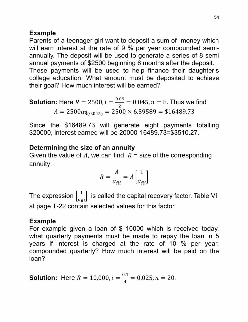
Example Parents of a teenager girl want to deposit a sum of money which will earn interest at the rate of 9 % per year compounded semi-annually. The deposit will be used to generate a series of 8 semi annual payments of $2500 beginning 6 months after the deposit. These payments will be used to help finance their daughter’s college education. What amount must be deposited to achieve their goal? How much interest will be earned?
Solution: Here = 2500, = .
= 0.045, 𝑛 = 8. Thus we find
= 2500𝑎 ( . ) = 2500 × 6.59589 = 16489.73
Since the $16489.73 will generate eight payments totalling $20000, interest earned will be 20000-16489.73=$3510.27. Determining the size of an annuity
Given the value of , we can find = size of the corresponding
annuity.
=
𝑎 = [
1
𝑎 ]
The expression [
] is called the capital recovery factor. Table VI
at page T-22 contain selected values for this factor. Example For example given a loan of $ 10000 which is received today, what quarterly payments must be made to repay the loan in 5 years if interest is charged at the rate of 10 % per year, compounded quarterly? How much interest will be paid on the loan?
Solution: Here = 10,000, = .
= 0.025, 𝑛 = 20.

55
Using the above formula
= 10000 [1
𝑎 ( . )] = 10000 × 0.06415 = 641.5.
There will be 20 payments totalling $12830, thus interest will be equal to $2830 on the loan.

56
Lecture 12,13
Chapter 10 Linear Programming:An Introduction
Basic concepts Linear Programming (LP) is a mathematical optimization technique. By “optimization” we mean a method or procedure which attempts to maximize or minimize some objective, e.g., maximize profit or minimize cost. In any LP problem certain decisions need to be made, these are represented by decision
variables 𝑥. The basic structure of a LP problem is either to maximize or minimize an objective function while satisfying a set of constraints.
1. Objective function is the mathematical representation of
overall goal stated as a function of decision variables 𝑥, examples are profit levels, total revenue, total cost, pollution levels, market share etc.
2. The Constraints, also stated in terms of 𝑥 , are conditions that must be satisfied when determining levels for the decision variables. They can be represented by equations or by inequalities (≤ and/or ≥ types).
The term Linear is due to the fact that all functions and constraints in the problem are linear. Example A simple linear programming problem is
Maximize 𝑧 = 4𝑥 + 2𝑥
Subject to 2𝑥 + 2𝑥 24
4𝑥 + 3𝑥 30.
The objective is to maximize 𝑧, which is stated as a linear function
of two decision variables 𝑥 and 𝑥 . In choosing values for 𝑥 and
𝑥 two constraints must be satisfied. The constraints are

57
represented by the two linear inequalities. A Scenario (a LP example) A firm manufactures two products, each of which must be
processed through two departments 1 and 2.
Product A Product B Weekly Labor Capacity
Department 1 3 h per unit 2 h per unit 120 h
Department 2 4 h per unit 6 h per unit 260 h
Profit Margins
$5 per unit $6 per unit
If 𝑥 and 𝑦 are the number of units produced and sold, respectively
of product A and B, then the total profit ‘𝑧’ is
𝑧 = 5𝑥 + 6𝑦 The restrictions in deciding the units produced are given by the inequalities:
3𝑥 + 2𝑦 120 (Department 1)
4𝑥 + 6𝑦 260 (Department 1)
We also know that 𝑥 and 𝑦 can not be negative. So the LP model which represents the stated problem is:
Maximize 𝑧 = 5𝑥 + 6𝑦
Subject to 3𝑥 + 2𝑦 120 (1)
4𝑦 + 6𝑦 260 (2)
𝑥 0 (3)
𝑦 0 (4) Inequalities (1) and (2) are called structural constraints, while (3) and (4) are non-negativity constraints.
58
Notably, the function 𝑧 is our objective function that needs to be maximized. Graphical Solutions When a LP model is stated in terms of 2 decision variables, it can be solved by graphical methods. Before discussing the graphical solution method, we will discuss the graphics of linear inequalities. Graphics of Linear Inequalities Linear inequalities which involve two variables can be represented graphically in two dimensions by a closed half space of a certain type of the certain plane. The half space consists of the boundary line representing the equality part of the inequality and all points on one side of the boundary line (representing the strict inequality). Graph the boundary which represents the equation. Determine the side that satisfy the strict inequality. System of Linear Inequalities In LP problems we will be dealing with system of linear inequalities. We will be interested to determine the solution set which satisfies all the inequalities in the system of constraints. Region of feasible solution The first step in graphical procedure is to identify the solution set for the system constraints. This solution set is called region of feasible solution. It includes all combinations of decision variables which satisfy the structural and non-negativity constraints. Corner point solution Given a linear objective function in a linear programming problem, the optimal solution will always include a corner point on the region of feasible solution. This will hold, irrespective of the slope of objective function and for either maximization or minimization

59
problems. We can use a method, called corner point method, to solve the linear programming problems. The corner point method for solving LP problems is as follows.
1. Graphically identify the region of feasible solutions. 2. Determine the coordinates of each corner point on the region
of feasible solution. 3. Substitute the coordinates of the corner points into the
objective function 𝑧 to determine the corresponding value of
𝑧. 4. The required solution occur at the corner point yielding,
(highest value of 𝑧 in maximization problems)/ (lowest value
of 𝑧 in minimization problems). Alternative Optimal Solutions There is a possibility of more than one optimal solutions in LP problem. Alternative optimal solution exists if the following two conditions are satisfied.
1. The objective function must be parallel to the constraint which forms an edge or boundary on the feasible region
2. The constraint must form a boundary on the feasible region in the direction of optimal movement of the objective function
Example (Page 437 in Book) Use corner-point method to solve:
Maximize 𝑧 = 20𝑥 + 15𝑥
Subject to 3𝑥 + 4𝑥 60 (1) 4𝑥 + 3𝑥 60 (2) 𝑥 10 (3) 𝑥 12 (4) 𝑥 , 𝑥 0 (5) Solution: The figure shows all the corner points of the given LP problem.
Corner point
𝑂(0,0) (0,12) 𝐵(10,0) 𝐶(4,12) 𝐷(10,
20
3 ) 𝐸(
60
7,60
7)
Value
of 𝑧 0 180 200 260 300 300

60
Optimal Solution occurs at the point D and E. In fact, any point along the line DE will give this optimal solution. Both the conditions for alternative optimal solutions were satisfied in this example. The objective function was parallel to the constraint (2) and the constraint (2) was a boundary line in the direction of the optimal movement of objective function.
No Feasible Solutions The system of constraints in an LP problem may have no points which satisfy all constraints. In such cases, there are no points in the solution set and hence the LP problem is said to have no feasible solution. Applications of Linear Programming
Diet Mix Model A dietician is planning the menu for the evening meal at a university dining hall. Three main items will be served, all having different nutritional content. The dietician is interested in providing at least the minimum daily requirement of each of three vitamins in this one meal. Following table summarizes the vitamin contents
61
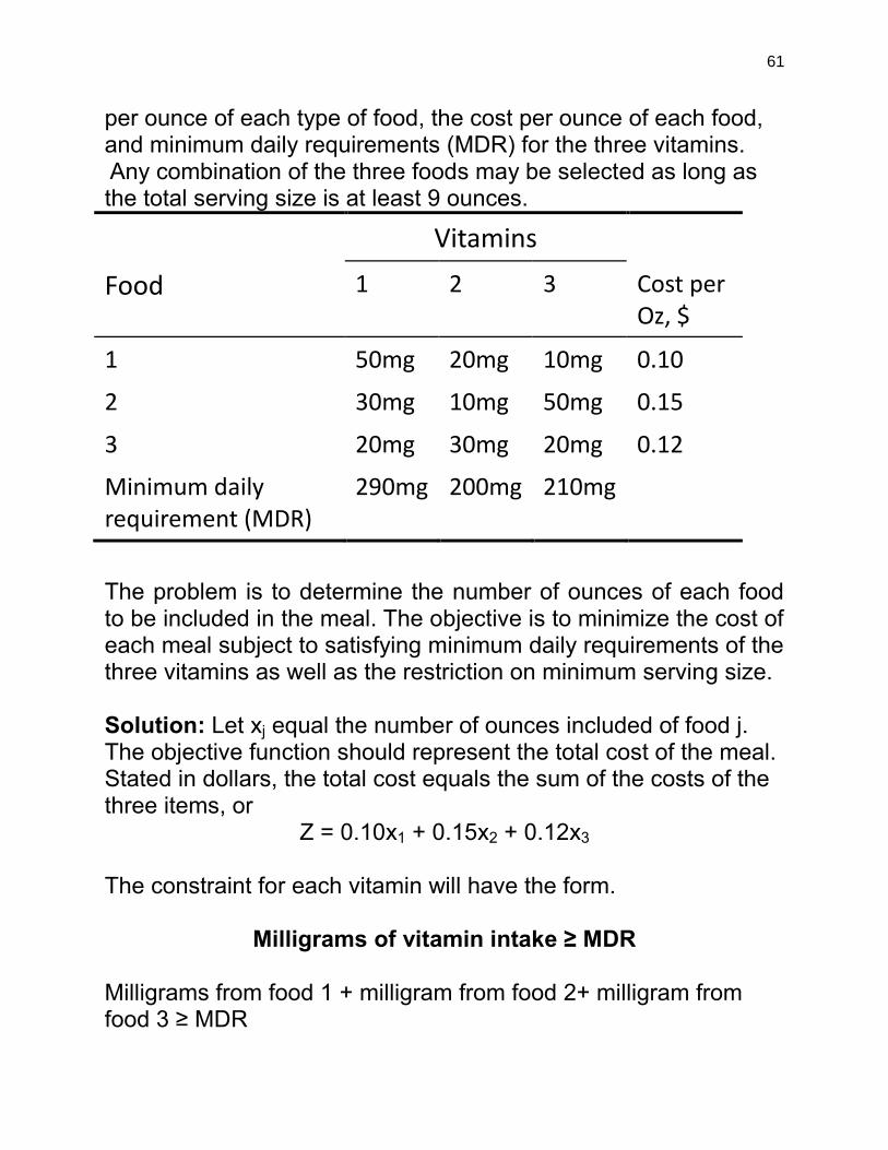
per ounce of each type of food, the cost per ounce of each food, and minimum daily requirements (MDR) for the three vitamins. Any combination of the three foods may be selected as long as the total serving size is at least 9 ounces.
Vitamins
Food 1 2 3 Cost per Oz, $
1 50mg 20mg 10mg 0.10
2 30mg 10mg 50mg 0.15
3 20mg 30mg 20mg 0.12
Minimum daily requirement (MDR)
290mg 200mg 210mg
The problem is to determine the number of ounces of each food to be included in the meal. The objective is to minimize the cost of each meal subject to satisfying minimum daily requirements of the three vitamins as well as the restriction on minimum serving size. Solution: Let xj equal the number of ounces included of food j. The objective function should represent the total cost of the meal. Stated in dollars, the total cost equals the sum of the costs of the three items, or
Z = 0.10x1 + 0.15x2 + 0.12x3
The constraint for each vitamin will have the form.
Milligrams of vitamin intake ≥ MDR
Milligrams from food 1 + milligram from food 2+ milligram from food 3 ≥ MDR
62
The constraints are, respectively, 50x1 + 30x2 + 20x3 ≥ 290 (vitamin 1) 20x1 + 10x2 + 30x3 ≥ 200 (vitamin 2) 10x1 + 50x2 + 20x3 ≥ 210 (vitamin 3) The restriction that the serving size be at least 9 ounces is stated as
x1 + x2+ x3 ≥ 9 (minimum serving size)
The complete formulation of the problem is as follows: Minimize z = 0.10x1 + 0.15x2 + 0.12x3
subject to 50x1 + 30x2 + 20x3 ≥ 290 20x1 + 10x2 + 30x3 ≥ 200 10x1 + 50x2 + 20x3 ≥ 210 x1 + x2 + x3 ≥ 9 x1 , x2, x3 ≥ 0 Transportation Model Transportation models are possibly the most widely used linear programming models. Oil companies commit tremendous resources to the implementation of such models. The classic example of a transportation problem involves the shipment of some homogeneous commodity from m sources of supply, or origins, to n points of demand, or destinations. By homogeneous we mean that there are no significant differences in the quality of the item provided by the different sources of supply. The item characteristics are essentially the same. Example (Highway Maintenance) A medium-size city has two locations in the city at which salt and sand stockpiles are maintained for use during winter icing and

63
snowstorms. During a storm, salt and sand are distributed from these two locations to four different city zones. Occasionally additional salt and sand are needed. However, it is usually impossible to get additional supplies during a storm since they are stockpiled at a central location some distance outside the city. City officials hope that there will not be back-to-back storms. The director of public works is interested in determining the minimum cost of allocating salt and sand supplies during a storm. Following table summarizes the cost of supplying 1 ton of salt or sand from each stockpile to each city zone. In addition, stockpile capacities and normal levels of demand for each zone are indicated (in tons) Solution: In formulating the linear programming model for this problem, there are eight decisions to make-how many tons should be shipped from each stockpile to each zone. Let xij equal the number of tons supplied from stockpile i to zone j. For example, x11 equals the number of tons supplied by stockpile 1 to zone 1. Similarly, x23 equals the number of tons supplied by stockpile 2 to zone 3. This double-subscripted variable conveys more information than the variables x1, x2,…, x8. Give this definition of the decision variables, the total cost of distributing salt and sand has the form:
Total Cost = 2x11 + 3x12 + 1.5x13 + 2.5x14 +4x21 + 3.5x22 +2.5x23 +3x24
This is the objective function that we wish to minimize. For stockpile 1, the sum of the shipments to all zones cannot exceed 900 tons, or
x11 + x12 + x13 + x14 ≤ 900 (stockpile 1)
The same constraint for stockpile 2 is

64
x21 + x22 + x23 + x24 ≤ 750 (stockpile 2) The final class of constraints should guarantee that each zone receives the quantity demanded. For zone 1, the sum of the shipments from stockpiles 1 and 2 should equal 300 tons, or
x11 + x21 = 300 (zone 1)
The same constraints for the other three zones are, respectively,
x12 + x22 = 450 (zone 2) x13 + x23 = 500 (zone 3) x14 + x24 = 350 (zone 4)
The complete formulation of the linear programming model is as follows: Minimize z = 2x11 + 3x12 + 1.5x13 + 2.5x14 + 4x11 + 3.5x22 +2.5x23 +3x24
Subject to x11 + x12 + x13 + x14 ≤ 900 x21 + x22 + x23 + x24 ≤ 750 x11 + x21 = 300 x12 + x22 = 450 x13 + x23 = 500 x14 + x24 = 350 x11 , x12 , x13 , x14 , x11 , x22 , x23 , x24 ≥ 0

65
Lecture 14,15,16,17
Chapter 11:The Simplex and Computer Solution
Methods
Simplex Preliminaries
Graphical solution methods are applicable to LP problems involving two variables. The geometry of three variable problems is very complicated, and beyond three variables, there is no geometric frame of reference, so we need some nongraphic Method. The most popular non-graphical procedure is called The Simplex Method. This is an algebraic procedure for solving system of equations where an objective function needs to be optimized. It is an iterative process, which identifies a feasible starting solution. The procedure then searches to see whether there exists a better solution. “Better” is measured by whether the value of the objective function can be improved. If better solution is signaled, the search resumes. The generation of each successive solution requires solving a system of linear equations. The search continues until no further improvement is possible in the objective function Requirements of the Simplex Method
1. All constraints must be stated as equations. 2. The right side of the constraint cannot be negative. 3. All variables are restricted to nonnegative values.
Most linear programming problems contain constraints which are inequalities. Before we solve by the simplex method, these inequalities must be restated as equations. The transformation

66
from inequalities to equations varies, depending on the nature of the constraints.
Transformation procedure for ≤ constraints For each “less than or equal to” constraint, a non-negative variable, called a slack variable, is added to the left side of the constraint. Note that the slack variables become additional variables in the problem and must be treated like any other variables. That means they are also subject to Requirement 3 that is, they cannot assume negative values.
For example 3𝑥 − 2𝑥 4 will be transformed as
3𝑥 + 2𝑥 + 𝑆 = 4. Transformation procedure for ≥ constraints For each “greater than or equal to” constraint, a non-negative variable E, called a surplus variable, is subtracted from the left side of the constraint. In addition, a non-negative variable A, called an artificial variable, is added to the left of side of the constraint. The artificial variable has no real meaning in the problem; its only function is to provide a convenient starting point (initial guess) for the simplex.
For example 𝑥 + 𝑥 10 will be transformed to
𝑥 + 𝑥 − 𝐸 + = 10. Transformation procedure for = constraints
For each “equal to” constraint, an artificial variable, is added to
the left of side of the constraint. For example 3𝑥 + 𝑥 = 10 will be
transformed to 3𝑥 + 𝑥 + = 10. Example Transform the following constraint set into the standard form required by the simplex method x1 + x2 ≤ 100, 2x1 + 3x2 ≥ 40, x1 – x2 = 25, x1, x2 ≥ 0

67
Solution: The transformed constraint set is x1 + x2 + S1 ≥ 100
2x1 + 3x2 – E2 + A2 ≤ 40 x1 – x2 + A3 = 25
x1, x2, S1, E2, A2, A3 ≥ 0
Note that each supplemental variable (slack, surplus, artificial) is assigned a subscript which corresponds to the constraint number. Also, the non-negativity restriction (requirement 3) applies to all supplemental variables. Example An LP problem has 5 decision variables; 10 (≤) constraints; 8 (≥) constraints; and 2 (=) constraints. When this problem is restated to comply with requirement 1 of the simplex method, how many variables will there be and of what types? Solution: There will be 33 variables: 5 decision variables, 10 slack variables associated with the 10 (≤) constraints, 8 surplus variables associated with the 8 (≥) constraints, and 10 artificial variables associated with the (≥) and (=) constraints.
5 + 10 + 8 + 10 = 33 Basic Feasible Solutions Let’s state some definitions which are significant to our coming discussions. Assume the standard form of an LP problem which has m structural constraints and a total of n’ decision and supplemental variables. Definition: A feasible solution is any set of values for the n’ variables which satisfies both the structural and non-negativity constraints.

68
Definition: A basic solution is any solution obtained by setting (n’–m) variables equal to 0 and solving the system of equations for the values of the remaining m variables. Definition: The (n’–m) variables which have been assigned values of 0, are called non-basic variables. The rest of the variables are called basic variables. Definition: A basic feasible solution is a basic solution which also satisfies the non-negativity constraints. Thus optimal solution can be found by performing a search of the basic feasible solution. The Simplex Method Before we begin our discussions of the simplex method, let’s provide a generalized statement of an LP model. Given the definitions xj = j-th decision variable cj = coefficient on j-th decision variable in the objective function. aij = coefficient in the i-th constraint for the j-th variable. bi = right-hand-side constant for the i-th constraint The generalized LP model can be stated as follows: Optimize (maximize or minimize) z = c1x1 + c2x2 + ... + cnxn
subject to a11x1 + a12x2 + ... + a1nxn (≤ , ≥ , =) b1 (1) a21x1 + a22x2 + ... + a2nxn (≤ , ≥ , =) b2 (2) ... am1x1 + am2x2 + ... + amnxn (≤ , ≥ , =)bm (m) x1 ≥ 0 x2 ≥ 0 ... xn ≥ 0

69
Solution by Enumeration Consider a problem having m (≤) constraints and n variables. Prior to solving by the simplex method, the m constraints would be changed into equations by adding m slack variables. This restatement results in a constraint set consisting of m equations and m + n variables. Example Solve the following LP problem. Maximize z = 5x1 + 6x2
subject to 3x1 + 2x2 ≤ 120 (1) 4x1 + 6x2 ≤ 260 (2) x1 , x2 ≥ 0 Solution: The constraint set must be transformed into the equivalent set. 3x1 + 2x2 + S1 = 120 4x1 + 6x2 + S2 = 260 x1 , x2 , S1 , S2 ≥ 0 The constraint set involves two equations and four variables. Of all the possible solutions to the constraint set, an optimal solution occurs when two of the four variables in this problem are set equal to zero and the system is solved for the other two variables. The question is, which two variables should be set equal to 0 (should be non-basic variables)? Let’s enumerate the different possibilities.
1. If S1 and S2 are set equal to 0, the constraint equations become
3x1 + 2x2 = 120 4x1 + 6x2 = 260 Solving for the corresponding basic variable x1 and x2 results in x1= 20 and x2 = 30
2. If S1 and x1 are set equal to 0, the system becomes 2x2 = 120

70
6x2 + S2 = 260 Solving for the corresponding basic variables x2 and S2 results in x2 = 60 and S2 = – 100
Following table summarizes the basic solutions, that is, all the solution possibilities given that two of the four variables are assigned 0 values.
Notice that solutions 2 and 5 are not feasible. They each contain
a variable which has a negative value, violating the non-negativity
restriction. However, solutions 1, 3, 4 and 6 are basic feasible
solutions to the linear programming problem and are candidates
for the optimal solution.
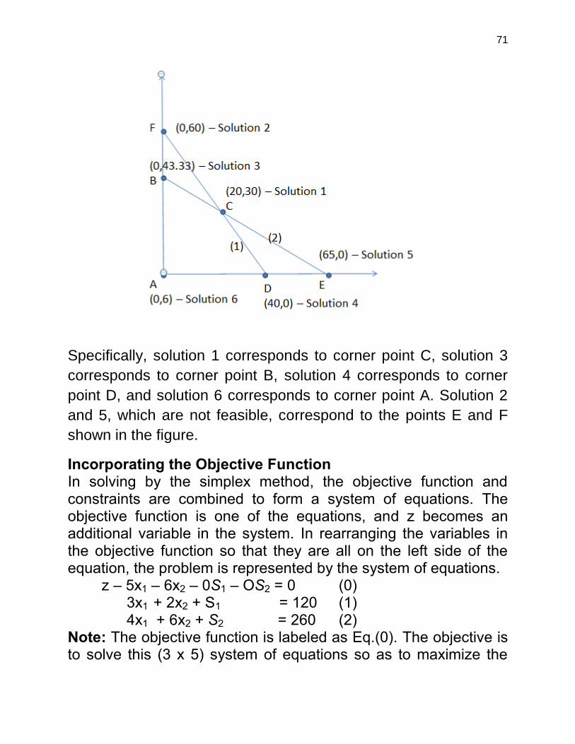
The following figure is the graphical representation of the set of constraints.
71
Specifically, solution 1 corresponds to corner point C, solution 3
corresponds to corner point B, solution 4 corresponds to corner
point D, and solution 6 corresponds to corner point A. Solution 2
and 5, which are not feasible, correspond to the points E and F
shown in the figure.
Incorporating the Objective Function In solving by the simplex method, the objective function and constraints are combined to form a system of equations. The objective function is one of the equations, and z becomes an additional variable in the system. In rearranging the variables in the objective function so that they are all on the left side of the equation, the problem is represented by the system of equations. z – 5x1 – 6x2 – 0S1 – OS2 = 0 (0) 3x1 + 2x2 + S1 = 120 (1) 4x1 + 6x2 + S2 = 260 (2) Note: The objective function is labeled as Eq.(0). The objective is to solve this (3 x 5) system of equations so as to maximize the
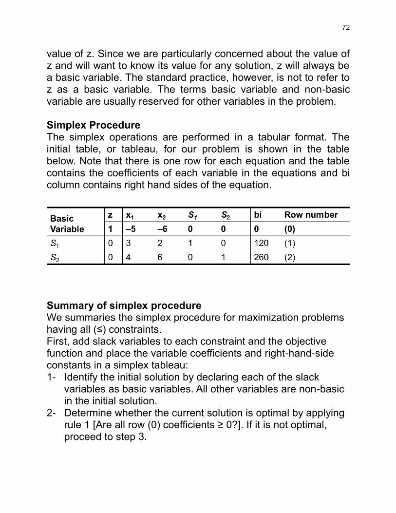
72
value of z. Since we are particularly concerned about the value of z and will want to know its value for any solution, z will always be a basic variable. The standard practice, however, is not to refer to z as a basic variable. The terms basic variable and non-basic variable are usually reserved for other variables in the problem. Simplex Procedure The simplex operations are performed in a tabular format. The initial table, or tableau, for our problem is shown in the table below. Note that there is one row for each equation and the table contains the coefficients of each variable in the equations and bi column contains right hand sides of the equation.
Summary of simplex procedure We summaries the simplex procedure for maximization problems having all (≤) constraints. First, add slack variables to each constraint and the objective function and place the variable coefficients and right-hand-side constants in a simplex tableau: 1- Identify the initial solution by declaring each of the slack
variables as basic variables. All other variables are non-basic in the initial solution.
2- Determine whether the current solution is optimal by applying rule 1 [Are all row (0) coefficients ≥ 0?]. If it is not optimal, proceed to step 3.

73
3- Determine the non-basic variable which should become a
basic variable in the next solution by applying rule 2 [most negative row (0) coefficient].
4- Determine the basic variable which should be replaced in the next solution by applying rule 3 (min bi/aik ratio where aik > 0)
5- Applying the Gaussian elimination operations to generate the new solution (or new tableau). Go to step 2.
Example(Page 488 in Book) Solve the following linear programming problem using the simplex method. Maximize z = 2x1 + 12x2 + 8x3
subject to 2x1 + 2x2 + x3 ≤ 100 x1 – 2x2 + 5x3 ≤ 80 10x1 + 5x2 + 4x3 ≤ 300 x1 , x2 , x3 ≥ 0 Solution: Detailed solution is in Book/Lectures. Maximization Problems with Mixed Constraints For a maximization problem having a mix of (≤, ≥, and =) constraints the simplex method itself does not change. The only change is in transforming constraints to the standard equation form with appropriate supplemental variables. Recall that for each (≥) constraint, a surplus variable is subtracted and an artificial variable is added to the left side of the constraint. For each (=) constraint, an artificial variable is added to the left side. An additional column is added to the simplex tableau for each supplemental variable. Also, surplus and artificial variables must be assigned appropriate objective function coefficients (c, values) Surplus variables usually re-assigned an objective function coefficient of 0. Artificial variables are assigned objective function coefficient of –M, where |M| is a very large number. This is to make the artificial variables unattractive in the problem.

74
In any linear programming problem, the initial set of basic variables will consist of all the slack variables and all the artificial variables which appear in the problem. Example (Page 491 in Book) Maximize z = 8x1 + 6x2
subject to 2x1 + x2 ≥ 10 3x1 + 8x2 ≤ 96 x1, x2 ≥ 0 We have a maximization problem which has a mix of a (≤) constraint and a (≥) constraint. Solution: (In Book/ Lectures)
Minimization Problems The simplex procedure is slightly different when minimization problems are solved. Aside from assigning artificial variables objective function coefficients of +M, the only difference relates to the interpretation of row (0) coefficients. The following two rules are modifications of rule 1 and rule 2. These apply for minimization problems. Rule 1A: Optimality Check in Minimization Problem. In a minimization problem, the optimal solution has been found if all row (0) coefficients for the variables are less than or equal to 0. If any row (0) coefficients are positive for non-basic variables, a better solution can be found by assigning a positive quantity to these variables. Rule 2A: New basic variable in minimization problem. In a minimization problem, the non-basic variable which will replace a current basic variable is the one having the largest positive row (0) coefficient. Ties may be broken arbitrarily.

75
Example (page 493 in Book) Solve the following linear programming problem using the simplex method. Minimize z = 5x1 + 6x2
subject to x1 + x2 ≥ 10 2x1 + 4x2 ≥ 24 x1 , x2 ≥ 0 Solution: This problem is first rewritten with the constraints expressed as equations, as follows: Minimize z = 5x1 + 6x2 + 0E1 + 0E2 + MA1 + MA2
subject to x1 + x2 – E1 + A1 = 10 2x1 + 4x2 – E2 + A2 = 24 x1, x2, E1, E2, A1, A2 ≥ 0
Basic Variables
z x1 x2 E1 E2 A1 A2
Need to Be Transformed to Zero bi Row
Number
1 –5 –6 0 0 –M –M 0 (0)
A1 0 1 1 –1 0 1 0 10 (1)
A2 0 2 4 0 –1 0 1 24 (2)
The initial tableau for this problem appears in above table. Note that the artificial variables are the basic variables in this initial solution. These –M coefficient in row (0) must be changed to 0 using row operations if the value of z is to be read from row (0).

76
In this initial solution the non-basic variables are x1, x2, E1, and E2. The basic variables are the two artificial variables with A1 = 10, A2 = 24, and z = 34M. Applying rule 1A, we conclude that this solution is not optimal. The x2 column becomes the new key column.
Applying rule 1A, we conclude that this solution is optimal. Therefore, z is minimized at a value of 52 when x1 = 8 and x2 = 2. Special Phenomena In Chapter 10, certain phenomena which can arise when solving LP problems were discussed. Specifically, the phenomena of alternative optimal solutions, no feasible solution, and unbounded solutions were presented. In this section we discuss the manner in which these phenomena occur when solving by the simplex method. Alternative Optimal Solutions An Alternative optimal solution results when the objective function is parallel to a constraint which binds in the direction of optimization. In two-variable problems we are made aware of alternative optimal solutions with the corner-point method when a “tie” occurs for the optimal corner point.

77
When using the simplex methods, alternative optimal solutions are indicated when 1- an optimal solution has been identified, 2- the row (0) coefficient for a non-basic variable equals zero. The first condition confirms that there is no better solution than the present solution. The presence of a 0 in row (0) for a non-basic variable indicates that the non-basic variable can become a basic variable (can become positive) and the current value of the objective function (known to be optimal) will not change. Example (page 491 in Book) Maximum z = 6x1 + 4x2
subject to x1 + x2 ≤ 5 3x1 + 2x2 ≤ 12 x1, x2 ≥ 0 Solution (In Lectures/Book)
No Feasible Solutions A problem has no feasible solution if there are no values for the variables which satisfy all the constraints. The condition of no feasible solution is signaled in the simplex method when an artificial variable appears in an optimal basis at a positive value. Let’s solve the following LP problem, which, by inspection, has no feasible solution.
Example (Page 499 in Book ) Maximize z = 10x1 + 20x2
subject to x + x2 ≤ 5 x1 + x2 ≥ 20 x1 , x2 ≥ 0 Solution: (In Lectures/Book)
Unbounded Solutions Unbounded solutions exist when there is an unbounded solution space. Improvement in the objective function occurs with

78
movement in the direction of the unbounded portion of the solution space. If at any iteration of the simplex method the aik
values are all 0 or negative for the variable selected to become the new basic variable, there is an unbounded solution for the LP problem. Example (Page 500-Book ) Maximize z = –2x1 + 3x2
subject to x1 ≤ 10 2x1 – x2 ≤ 30 x1, x2 ≥ 0 Solution: (In Lectures/Book) The Dual Problem Every LP problem has a related problem called the dual problem or, simply, the dual. Given an original LP problem, referred to as the primal problem, or primal, the dual can be formulated from information contained in the primal. Given an LP problem, its solution can be determined by solving either the original problem or its dual. Formulation of the Dual The parameters and structure of the primal provide all the information necessary to formulate the dual. The following problem illustrates the formulation of a maximization problem and the dual of the problem. 1- The primal is a maximization problem and the dual is a
minimization problem. The sense of optimization is always opposite for corresponding primal and dual problems.
2- The primal consists of two variables and three constraints and the dual consists of three variables and two constraints. The number of variables in the primal always equals the number of constraints in the dual. The number of constraints in the primal always equals the number of variables in the
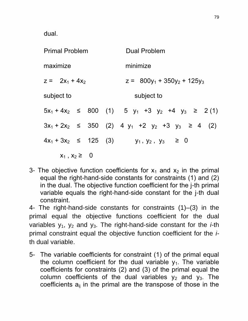
79
dual.
Primal Problem Dual Problem maximize minimize z = 2x1 + 4x2 z = 800y1 + 350y2 + 125y3
subject to subject to 5x1 + 4x2 ≤ 800 (1) 5 y1 +3 y2 +4 y3 ≥ 2 (1) 3x1 + 2x2 ≤ 350 (2) 4 y1 +2 y2 +3 y3 ≥ 4 (2)
4x1 + 3x2 ≤ 125 (3) y1 , y2 , y3 ≥ 0 x1 , x2 ≥ 0 3- The objective function coefficients for x1 and x2 in the primal
equal the right-hand-side constants for constraints (1) and (2) in the dual. The objective function coefficient for the j-th primal variable equals the right-hand-side constant for the j-th dual constraint.
4- The right-hand-side constants for constraints (1)–(3) in the
primal equal the objective functions coefficient for the dual
variables y1, y2 and y3. The right-hand-side constant for the i-th
primal constraint equal the objective function coefficient for the i-
th dual variable.
5- The variable coefficients for constraint (1) of the primal equal the column coefficient for the dual variable y1. The variable coefficients for constraints (2) and (3) of the primal equal the column coefficients of the dual variables y2 and y3. The coefficients aij in the primal are the transpose of those in the

80
dual. That is, the row coefficients in the primal become column coefficients in the dual, and vice versa.
The following table summarizes the symmetry of the two types of problems and their relationships.
Relationship 4 and 8 indicate that an equality constraint in one problem corresponds to an unrestricted variable in the other problem. An unrestricted variable can assume a value which is positive, negative, or 0. Similarly, relationship 3 and 7 indicate that a problem may have non-positive variables (for example xj = 0). Unrestricted and non-positive variables appear to violate the third requirement of the simplex method, the non-negativity restriction. There are methods which allow us to adjust the formulation to

81
satisfy the third requirement. Example Given the primal problem find the corresponding dual problem. Maximize z = 10x1 + 20x2 + 15x3 + 12x4
subject to x1 + x2 + x3 + x4 ≥ 100 (1)
2x1 – x3 + 3x4 ≤ 140 (2)
x1 + 4x2 – 2x4 = 50 (3)
x1, x3, x4 ≥ 0
x2 unrestricted
Solution: The corresponding dual is
Maximize z = 100y1 + 140y2 + 50y3
subject to y1 + 2y2 + y3 ≤ 10
y1 + 4y3 = 20
y1 – y2 – ≤ 15
y1 + 3y2 – 2y3 ≤ 12
y1 ≥ 0
y2 ≤ 0
y3 unrestricted
Primal-Dual Solutions It was indicated earlier that the solution to the primal problem can be obtained from the solution to the dual problem and vice versa. Let’s illustrate this by example. Consider the primal problem.

82
Maximize z = 5x1 + 6x2
subject to 3x1 + 2x2 ≤ 120 (1)
4x1 + 6x2 ≤ 260 (2)
x1 , x2 ≥ 0
The corresponding dual is Minimize z = 120y1 + 260y2 Subject to 3y1 + 4y2 ≥ 5 2y1 + 6y2 ≥ 6 y1 , y2 ≥ 0
The following table presents the final (optimal) tableau for the primal and dual problem.
83
Note from this tableau that z is minimized at a value of 280 when y1 =
3/5 and y2 =
4/5. Let’s illustrate how the solution to each
problem can be read from the optimal tableau of the corresponding dual problem. Primal-Dual Property 1
1. If feasible solutions exist for both the primal and dual problems, then both problems have an optimal solution for which the objective function values are equal.
2. A peripheral relation-ship is that if one problem has an unbounded solution, its dual has no feasible solution.
Primal-Dual Property 2 The optimal values for decision variables in one problem are read from row (0) of the optimal tableau for the other problem.
1. The optimal values y1 = 3/5 and y2 =
4/5 are read from above
table as the row (0) coefficients for the slack variables S1 and S2.
2. The optimal values x1 = 20 and x2 = 30 are read from above table as the negatives of the row (0) coefficients for the surplus variables E1 and E2.
3. These values can be read, alternatively, under the respective artificial variables, as the portion (term) of the row (0) coefficient not involving M.

84
Lecture 18,19,20
Chapter12: Transportation and Assignment Models
The aim of this chapter is to provide an overview of several extensions of the basic linear programming model. It will Include a discussion of the assumptions, distinguishing characteristics, methods of solution, and applications of the transportation model and the assignment model. The transportation model The classic transportation model involves the shipment of some homogeneous commodity from a set of origins to a set of destinations. Each origin represents a source of supply for the commodity; each destination represents a point of demand for the commodity. Assumption-1 The standard model assumes a homogeneous commodity. This first assumption implies that there are no significant differences in the characteristics of the commodity available at each origin. This suggests that unless other restrictions exist, each origin can supply units to any of the destinations. Assumption-2 The standard model assumes that total supply and total demand are equal. This second assumption is required by a special solution algorithm for this type of model. Let’s state the generalized transportation model associated with the structure shown in the figure given below.

85
If xij = number of units distributed from origin i to destination j cij = contribution to the objective function from distributing one unit
from origin i to destination j Si = number of units available at origin i dj = number of units demanded at destination j m = number of origins n = number of destinations

86
the generalized model can be stated as follows: Minimize z = c11x11 + c12x12 + . . . + c1nx1n + c21x21 + c22x22 + . . . (or maximize) . . . + c2nx2n + . . . + cmnxmn
Subject to x11 + x12 + . . . +x1n = S1
x21 + x22 + . . . + x2n = S2 supply
. . . Constraints . . . xm1 + xm2 + . . . + xmn = Sm
x11 + x21 . . . + xm1 = d1
x12 + x22 + . . . + xm2 = d2
. . . demand . . . constraints x1n + x2n + . . . + xmn = dn
xij ≥ 0 for all i and j Implicit in the model is the balance between supply and demand.
S1 + S2 + . . . + Sm = d1 + d2 + . . . + dn
The transportation model is a very flexible model which can be applied to the problems that have nothing to do with the distribution of commodities. Example (Job Placement Screening) A job placement agency works on a contract basis with employers. A computer manufacturer is opening a new plant and has contracted with the placement agency to process job applications for prospective employees. Because of the uneven demands in workload at the agency, it often uses part-time personnel for the purpose of processing applications. For this particular contract, five placement analysts must be hired. Each
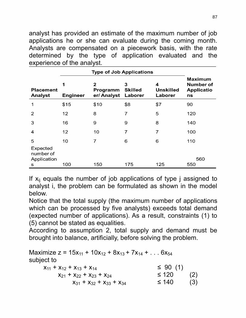
87
analyst has provided an estimate of the maximum number of job applications he or she can evaluate during the coming month. Analysts are compensated on a piecework basis, with the rate determined by the type of application evaluated and the experience of the analyst.
If xij equals the number of job applications of type j assigned to analyst i, the problem can be formulated as shown in the model below. Notice that the total supply (the maximum number of applications which can be processed by five analysts) exceeds total demand (expected number of applications). As a result, constraints (1) to (5) cannot be stated as equalities. According to assumption 2, total supply and demand must be brought into balance, artificially, before solving the problem. Maximize z = 15x11 + 10x12 + 8x13 + 7x14 + . . . 6x54
subject to x11 + x12 + x13 + x14 ≤ 90 (1)
x21 + x22 + x23 + x24 ≤ 120 (2)
x31 + x32 + x33 + x34 ≤ 140 (3)

88
x41 + x42 + x43 + x44 ≤ 100 (4)
x51 + x52 + x53 + x54 ≤ 110 (5)
x11 +x21 +x31 +x41 +x51 = 100 (6)
x12 +x22 +x32 +x42 +x52 = 150 (7)
x13 +x23 +x33 +x43 +x53 = 175 (8)
x14 +x24 +x34 + x44 +x54 = 125 (9) xij ≥ 0 for all
i and j Solutions to transportation models The simplex method can be used to solve transportation models. However, methods such as the stepping stone algorithm and a dual-based enhancement called the MODI method prove much more efficient.
Initial solutions The increased efficiency can occur during two different phases of solution:
1. Determination of the initial solution 2. Progress from the initial solution to the optimal
solution With the simplex method the initial solution is predetermined by the constraint structure. The initial set of basic variables will always consist of the slack and artificial variable in the problem. With transportation models the stepping stone algorithm (or the MODI method) will accept any feasible solution as a starting point. Consequently, various approaches to finding a good starting solution have been proposed. These include the northwest corner method, the least cost method, and Vogel’s approximation method.
Example Consider the data contained in the table for a transportation problem involving three origins and three destinations.

89
Assume that the elements in the body of the table represent the costs of shipping a unit from each origin to each destination. Also shown are the supply capacities of the three origins and the demands at each destination. Conveniently, the total supply and total demand are equal to one another. The problem is to determine how many units to ship from each origin to each destination so as to satisfy the demands at the three destinations while not violating the capacities of the three origins. The objective is to make these allocations in such a way as to minimize total transportation costs. Solution: We will solve this problem using two special algorithms. We will illustrate the northwest corner method, which can be used to determine an initial (starting) solution. Next, we illustrate the stepping stone algorithm, which can be used to solve these types of models. Before we begin these examples, let’s discuss come requirements of the stepping stone algorithm. Requirements of stepping stone algorithm 1- Total supply = Total demand
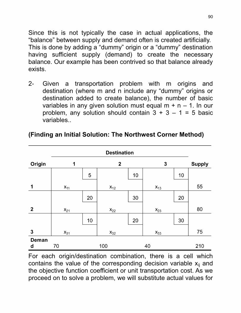
90
Since this is not typically the case in actual applications, the “balance” between supply and demand often is created artificially. This is done by adding a “dummy” origin or a “dummy” destination having sufficient supply (demand) to create the necessary balance. Our example has been contrived so that balance already exists. 2- Given a transportation problem with m origins and
destination (where m and n include any “dummy” origins or destination added to create balance), the number of basic variables in any given solution must equal m + n – 1. In our problem, any solution should contain 3 + 3 – 1 = 5 basic variables..
(Finding an Initial Solution: The Northwest Corner Method)
For each origin/destination combination, there is a cell which contains the value of the corresponding decision variable xij and the objective function coefficient or unit transportation cost. As we proceed on to solve a problem, we will substitute actual values for

91
the xij’s in the table as we try different allocations. The northwest corner method is a popular technique for arriving at an initial solution. The technique starts in the upper left-hand cell (northwest corner) of a transportation table and assigns units from origin 1 to destination 1. Assignments are continued in such a way that the supply at origin 1 is completely allocated before moving on to origin 2. The supply at origin 2 is completely allocated before moving to origin 3, and so on. Similarly, a sequential allocation to the destinations assures that the demand at destination 1 is satisfied before making allocations to destination 2; and so forth. The following table indicates the initial solution to our problem as derived using the northwest corner method.
Table 1

92
1- Starting in the northwest corner, the supply at origin 1 is 55
and the demand at destination 1 is 70. Thus, we allocate supply at origin 1 in an attempt to satisfy the demand at destination 1 (x11 = 55).
2- When the complete supply at origin 1 has been allocated,
the next allocation will be from origin 2. The allocation in cell (1, 1) did not satisfy the demand at destination 1 completely. Fifteen additional units are demanded. Comparing the supply at origin 2 with the remaining demand at destination 1, we allocate 15 units from origin 2 to destination 1 (x21 = 15). This allocation completes the needs of destination 1, and the demand at destination 2 will be addressed next.
3- The last allocation left origin 2 with 65 units. The demand at
destination 2 is 100 units. Thus, we allocate the remaining supply of 65 units to destination 2 (x22 = 65). The next allocation will come from origin 3.
4- The allocation of 65 units from origin 2 left destination 2 with
unfulfilled demand of 35 units. Since origin 3 has a supply of 75 units, 35 units are allocated to complete the demand for that destination (x32 = 35). Thus, the next allocation will be destination 3.
5- The allocation of 35 units from origin 3 leaves that origin with 40 remaining units. The demand at destination 3 also equals 40; thus, the final allocation of 40 units is made from origin 3 to destination 3 (x33 = 40).
Notice in the above table that all allocations are circled in the appropriate cells. These represent the basic variables for this solution. There could be five basic variables (m + n – 1) to satisfy

93
the requirement of the stepping stone algorithm. The recommended allocations and associated costs for this initial solution are summarized in the following table.
Stepping Stone Algorithm
Step 1: Determine the improvement index for each non-basic variable (cell). As we examine the effects of introducing one unit of a non-basic variable, we focus upon two marginal effects:
1. What adjustments must be made to the values of the current basic variables (in order to continue satisfying all supply and demand constraints)?
2. What is the resulting change in the value of the objective function?

94
1) To illustrate, focus upon the above table. Cell (1,2) has no allocation in the initial solution and is a non-basic cell. The question we want to ask is what trade-offs (or adjustments) with the existing basic variables would be required if 1 unit is shipped from origin 1 to destination 2?
2) Summarizing, to compensate for adding a unit to cell (1, 2), shipments in cell (1, 1) must be decreased by 1 unit, shipments in cell (2, 1) must be increased by 1 unit, and shipments in cell (2,2) must be decreased by 1 unit.
3) The next question is, What is the marginal effect on the
value of the objective function? 4) For each cell (i, j) receiving an increased allocation of 1 unit,
costs increase by the corresponding cost coefficient (cij). 5) Similarly, costs decrease by the value of the cost coefficient
wherever allocations have been reduced by 1 unit. 6) These effects are summarized in the following table.

95
The net (marginal) effect associated with allocating 1 unit from origin 1 to destination 2 is to reduce total cost by $5.00. This marginal change in the objective function is called the improvement index for cell (1, 2). Trace a “closed path” which begins at the unoccupied cell of interest; moves alternately in horizontal and vertical directions, pivoting only on occupied cells, and terminates on the unoccupied cell. The pluses and minuses indicate the necessary adjustments for satisfying the row (supply) and column (demand) requirements. Note: The direction in which the path is traced is not important. Tracking the path clockwise or counter-clockwise will result in the same path and identical adjustments. Once the closed path has been identified for a non-basic cell, the improvement index for that cell is calculated by adding all objective function coefficient for cells in plus positions on the path

96
and subtracting corresponding objective function coefficients for cells in negative positions on the path.

97
We can also make the above table for cell (3,1) and cell (2,3). (See Lectures)
• The above table summarizes the closed paths and improvement indices for all non-basic cells in the initial solution.
• Verify these path and values for the improvement indices to make sure you understand what we have been discussing.
Step 2: If a better solution exists, determine which variable (cell) should enter the basis. An examination of the improvement indices in the above table indicates that the introduction of three of the four non-basic variables would lead to a reduction in total costs. For minimization problems, a better solution exists if there are any negative improvement indices. An optimal solution has been found when all improvement indices are non-negative. For maximization problems a better solution has been found when all improvement indices are non-positive.

98
As in the simplex method, we select the variable (cell) which leads to the greatest marginal improvement in the objective function.
Entering Variable
• For minimization problems, the entering variable is identified
as the cell having the largest negative improvement index
(ties may be broken arbitrarily).
• For maximization problems, the entering variable is the cell
having the largest positive improvement index.
In our example, cell (2, 3) or x23, is selected as the entering
variable.

99
Step 3: Determine the departing variable and the number of units to assign the entering variable.
This step is performed by returning to the closed path associated with the incoming cell.
The above table shows the closed path for cell (2, 3).
The stepping stone algorithm parallels the simplex exactly, we need to determine the number of units we can assign to cell (2, 3) such that the value of one of the current basic variables is driven to 0.
From the above table we see that only two basic variables decrease in values additional units are allocated to cell (2, 3): cells (2, 2) and (3, 3), both of which are in minus positions on the closed path.
The question is which of these will go to 0 first as more units are added to cell (2, 3).
We can reason that when the 40th
unit is added to cell (2, 3), the value for cell (2, 2) reduces to 25, the value for cell (3, 2) increases to 75, and the value of cell (3, 3) goes to 0.
Departing variable The departing variable is identified as the smallest basic variable in a minus position on the closed path for the entering variable.
Number of units to assign entering variable The number of units equals the size of the departing variable (the smallest value in a minus position). Step 4: Develop the new solution and return to step 1. Again referring to the closed path for the incoming cell (2, 3), add

100
he quantity determined in step 3 to all cells in plus positions and subtract this quantity from those in minus positions. Thus, given that the entering variable x23 = 40 from step 3, the cells on the closed path are adjusted, leading to the second solution shown in the following table. When you determine a new solution you should check the allocations along each row and column to make sure that they add to the respective supply and demand values. Also, make sure that there are m + n – 1 basic variables. It can be seen in the following table that both of the above requirements are satisfied.
One other piece of information which is of interest is the new value of the objective function. We can multiply the value of each basic variable times its corresponding objective function coefficient and sum, as we did in the above table.

101
Given that the original value of the objective function was $4,425 and that each unit introduced to cell (2, 3) decreases the value of the objective by $20, introducing 40 units to cell (2, 3) results in a new value for total cost of.
z = $4,425 – (40) ($20) = $4,425 – $800 = $3,625
The following tables summarize the remaining steps in solving this problem. See whether you can verify these steps and the final result.
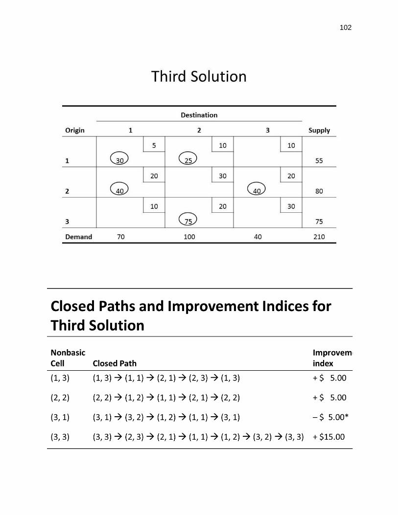
102

103
Since all improvement indices are nonnegative in the above table, we conclude that the solution in the above table is optimal. That

104
is, total cost will be minimized at a value of $3,350 if 55 units are shipped from origin 1 to destination 2 40 units from origin 2 to destination 1 40 units from origin 2 to destination 3 350 units from origin 3 to destination 1 45 units from origin 3 to destination 2
Alternative optimal solution Given that an optimal solution has been identified for a transportation model, alternative optimal solutions exist if any improvement indices equal 0. If the conditions for optimality exist, allocation of units to cells having improvement indices of 0 results is no change in the (optimal) value for the objective function. In our optimal solution, the above table indicates that allocation of units to cell (2, 2) would result in no change in the total cost.
The Assignment Model and Methods of Solution A special case of the transportation model is the assignment model. This model is appropriate in problems which involve the assignment of resources to tasks (e.g, assign n persons to n different tasks or jobs). As the special structures of the transportation model allows for solution procedures which are more efficient than the simplex method, the structure of the assignment model allows for solution methods more efficient than the transportation method. General Form and Assumptions The general assignment problem involves the assignment of n resources (origins) to n tasks (destinations).Typical examples of assignment problems include the assignment of salespersons to sales territories, airline crews to flights, ambulance units to calls for service, referees and official to sports events, and lawyers within a law firm to cases or clients. The objective in making assignment can be one of minimization or maximization (e.g., minimization of total time required to complete n tasks or

105
maximization of total profit from assigning salespersons to sales territories). The following assumptions are significant in formulating assignment models. Assumption 1 Each resource is assigned exclusively to one task. Assumption 2 Each task is assigned exactly one resource. Assumption 3 For purposes of solution, the number of resources available for assignment must equal the number of tasks to be performed. General Form
If
𝑥 = 1 if resource i is assigned to task j
𝑥 = 0 if resource i is not assigned to task j
cij = Objective function contribution if resource i is assigned to
task j n = number of resources and number of tasks. The generalized assignment model is shown as follows.

106
Notice for this model that the variables are restricted to the two values of 0 (non-assignment of the resource) or 1 (assignment of the resource). This restriction on the values of the variables is quite different from the other linear programming models we have examined. Constraints (1) to (n) ensure that each resource is assigned to one task only. Constraints (n + 1) to (n + n) ensure that each task is assigned exactly to one resource. According to assumption 3, the number of resources must equal the number of tasks for purposes of solving the problem. This condition might have to be artificially imposed for a given problem. Finally, notice that all right-hand-side constants, which are equivalent to si and dj values in the transportation model, equal 1. The supply of each resource is 1 unit and the demand for each task is 1 unit.

107
Example (NCAA Referee Assignments)
This problem can be formulated as an assignment model. Let
𝑥 = 1 if team i is assigned to tournament j
0 if team i is not assigned to tournament j The problem formulation is as follows:

108
Constraints (1) to (4) assure that each team of officials is assigned to one tourney site only; constraints (5) to (8) assure that each site is assigned exactly one team of officials. Solution Methods Assignment models can be solved using various procedures. These include total enumeration of all solutions, 0 – 1 programming methods, the simplex method, transportation methods (stepping stone), and special-purpose algorithms. These techniques are listed in an order reflecting increasing efficiency. One of the most popular methods is the Hungarian method. The Hungarian Method The Hungarian method is based on the concept of opportunity

109
costs. There are three steps in implementing the method.
1) An opportunity cost table is constructed from the table of assignment costs.
2) It is determined whether an optimal assignment can be made. 3) If an optimal assignment cannot be made, the third step
involves a revision of the opportunity cost table. Let’s illustrate the algorithm with the following example. Example (Court Scheduling) A court administration is in the process of scheduling four court dockets. Four judge are available to be assigned, one judge to each docket. The court administration has information regarding the type of cases on each of the dockets as well as data, indicating the relative efficiently of each of the judges in processing different types of court cases.
Estimated Days to Clear Docket
Based upon this information, the court administrator has
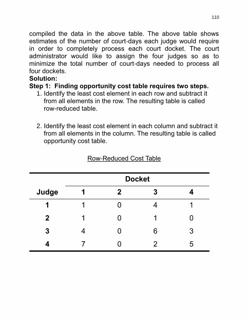
110
compiled the data in the above table. The above table shows estimates of the number of court-days each judge would require in order to completely process each court docket. The court administrator would like to assign the four judges so as to minimize the total number of court-days needed to process all four dockets. Solution: Step 1: Finding opportunity cost table requires two steps.
1. Identify the least cost element in each row and subtract it from all elements in the row. The resulting table is called row-reduced table.
2. Identify the least cost element in each column and subtract it from all elements in the column. The resulting table is called opportunity cost table.
Row-Reduced Cost Table

111
Opportunity Cost Table
Step 2: Determine whether an optimal assignment can be
made:
• Draw the straight lines (horizontally and vertically) through opportunity cost table in such a way as to minimize the number of lines necessary to cover all zero entries.
• If number of lines equals either the number of rows or number of columns in the table, an optimal solution can be found.
• Otherwise, opportunity cost table must be revisited. Step 3: Revise the opportunity cost table.
• Identify the smallest number in the table not covered by straight lines.
• Subtract this number from all the numbers not covered by straight lines and add this number to all numbers lying at the intersection of any two lines.

112
Revised Opportunity Cost Table
Step 2: Determine whether an optimal assignment can be
made:
As number of lines now of rows, optimal assignment is possible. How to make optimal assignment?
• Select a row or column in which is only one zero and make an assignment to that cell.
• Cross out that row and column and repeat step 1.

113
Optimal Assignments
• Select a row/column in which there is only one zero.
• Make an assignment to that cell.
• There is only one zero in column 4, thus first assignment is judge 2 to docket 4.
• Since no further assignment is possible in row 2 or column 4, we cross them off.
• Again find the row or column in which there is only one zero and repeat the steps above.
• Continue until all the judges are assigned to respective dockets.
Summary of the Hungarian Method Step 1: Determine the opportunity cost table.

114
a- Determine the row-reduced cost table by subtracting the least cost element in each row from all elements in the same row.
b- Using the row-reduced cost table, identify the least cost
element in each column, and subtract from all elements in that column.
Step 2: Determine whether or not an optimal assignment can be
made. Draw the minimum number of straight lines necessary to cover all zero elements in the opportunity cost table. If the number of straight lines is less than the number of rows (or columns) in the table, the optimal assignment cannot be made. Go to step 3. If the number of straight lines equals the number of rows (columns), the optimal assignments can be identified.
Step 3: Revise the opportunity cost table. Identify the smallest
element in the opportunity cost table not covered by a straight line.
a- Subtract this element from every element not covered
by a straight line. b- Add this element to any element(s) found at the
intersection of two straight lines. c- Go to step 2. The Hungarian method can be used when the objective function is to be maximized. Two alternative approaches can be used in this situation. The signs on the objective function coefficients can be changed, and the objective function can be minimized, or opportunity costs can be determined by subtracting the largest element (e.g., profit) in a row or column rather than the smallest element.

115
Lecture 21,22
Chapter 15: Differentiation This is the first of six chapters which examine the calculus and its application to business, economics, and other areas of problem solving. Two major areas of study within the calculus are differential calculus and integral calculus. Differential calculus focuses on rates of change in analyzing a situation. Graphically, differential calculus solves of following problem: Given a function whose graph is a smooth curve and given a point in the domain of the function, what is the slope of the line tangent to the curve at this point.
Limits
Two concepts which are important in the theory of differential and integral calculus are the limit of a function and continuity. Limits of Functions In the calculus there is often an interest in the limiting value of a function as the independent variable approaches some specific real number. This limiting value, when it exists, is called limit. The notation
lim
𝑓(𝑥) = 𝐿
is used to express the limiting value of a function. When
investigating a limit, one is asking whether 𝑓(𝑥) approaches a
specific value 𝐿 as the value of 𝑥 gets closer and closer to 𝑎. Notation of Limits The notation
lim
𝑓(𝑥) = 𝐿
represents the limit of 𝑓(𝑥) as 𝑥 approaches ‘𝑎’ from the left (left-hand limit). The notation

116
lim
𝑓(𝑥) = 𝐿
represents the limit of 𝑓(𝑥) as 𝑥 approaches ‘𝑎’ from the right (right-hand limit).
If the value of the function approaches the same number 𝐿 as 𝑥
approaches ‘𝑎’ from either direction, then the limit is equal to 𝐿. Test For Existence Of Limit
If lim 𝑓(𝑥) = 𝐿=lim 𝑓(𝑥) then
lim 𝑓(𝑥) = 𝐿
If the limiting values of 𝑓(𝑥) are different when 𝑥 approaches 𝑎 from each direction, then the function does not approach a limit as
𝑥 approaches 𝑎. Example
Determine whether the lim 𝑥 exists or not? Solution: In order to determine the limit let’s construct a table of assumed value for x and corresponding values for f(x). The following table indicates these values.

117
Note that the value of x=2 has been approached from both the left and the right. From either direction, f(x) is approaching the same value, 8. Note: For more examples, consult lectures and book.
Properties Of Limits And Continuity
1. If 𝑓(𝑥) = 𝑐, where c is real, then lim 𝑓(𝑥) = 𝑐
2. If 𝑓(𝑥) = 𝑥 , where 𝑛 is a positive integer, then
lim 𝑥 = 𝑎
3. If f(x) has a limit as 𝑥 𝑎 and c is any real number, then
lim 𝑐. 𝑓(𝑥) = 𝑐. lim 𝑓(𝑥) 4. If lim 𝑓(𝑥)and lim 𝑔(𝑥) exist, then
lim 𝑓(𝑥) ± 𝑔(𝑥) = lim 𝑓(𝑥) ± lim 𝑔(𝑥) 5. If lim 𝑓(𝑥), lim 𝑔(𝑥)exist, then
lim 𝑓(𝑥). 𝑔(𝑥) = lim 𝑓(𝑥) . lim 𝑔(𝑥) 6. If lim 𝑓(𝑥) and lim 𝑔(𝑥) exist, then
lim
𝑓(𝑥)
𝑔(𝑥)=
lim
𝑓(𝑥)
lim
𝑔(𝑥)
Limits and Infinity Frequently there is an interest in the behavior of a function as the independent variable becomes large without limit (“approaching” either positive or negative infinity). Horizontal Asymptote The line y = a is a horizontal asymptote of the graph of f if and only if

118
lim
𝑓(𝑥) = 𝑎
Note: See detailed discussion and examples in books. Vertical Asymptote The line x = a is a vertical asymptote of the graph of f if and only if
lim
𝑓(𝑥) = ∞
Continuity In an informal sense, a function is described as continuous if it can be sketched without lifting your pen or pencil from the paper (i.e., it has no gaps, no jumps, and no breaks). A function that is not continuous is termed as discontinuous. Continuity at a Point A function f is said to be continuous at x = a if 1- the function is defined at x = a, and
2- lim 𝑓(𝑥) = 𝑓(𝑎) Examples
Determine that 𝑓(𝑥) = 𝑥 is continuous at 𝑥 = 2. Solution: Since
lim
𝑥 = 𝑓(2) = 8.
Thus 𝑓 is continuous at 𝑥 = 2. Average Rate of Change and the Slope The slope of a straight line can be determined by the two-point formula

119
12
12
xx
yy
x
ym
The slope provides an exact measure of the rate of change in the value of y with respect to a change in the value of x. With nonlinear functions the rate of change in the value of y with respect to a change in x is not constant. One way of describing nonlinear functions is by the average rate of change over some interval. In moving from point A to point B, the change in the value of x is (x + Δx) – x, or Δx. The associated change in the value of y is
Δy = f(x + Δx) – f(x)
The ratio of these changes is. Δ𝑦
Δ𝑥=
𝑓(𝑥 + Δ𝑥) − 𝑓(𝑥)
Δ𝑥
The above equation is sometimes referred to as the difference quotient. What Does The Difference Quotient Represent Given any two points on a function f having coordinates
𝑥, 𝑓(𝑥) and (𝑥 + 𝛥𝑥), 𝑓(𝑥 + 𝛥𝑥) , the difference quotient represents.
1. The average rate of change in the value of y with respect to the change in x while moving from
𝑥, 𝑓(𝑥) 𝑜 (𝑥 + 𝛥𝑥), 𝑓(𝑥 + 𝛥𝑥) 2. The slope of the secant line connecting the two points.
Examples Find the general expression for the difference quotient of the
function 𝑦 = 𝑓(𝑥) = 𝑥 . Find the slope of the line connecting (-2, 4) and (3, 9) using the two-point formula. Find the slope in part (b) using the expression for the difference quotient found in part (a). Solution (In Lectures)

120
The Derivative DEFINITION: Given a function of the form y = f(x), the derivative of the function is defined as
𝑦
𝑥= lim
Δ𝑦
Δ𝑥= lim
𝑓(𝑥 + Δ𝑥) − 𝑓(𝑥)
Δ𝑥
If this limit exists. Comments About The Derivative
i. The above equation is the general expression for the derivative of the function f.
ii. The derivative represents the instantaneous rate of change in the dependent variable given a change in the independent
variable. The notation 𝑦/ 𝑥 is used to represent the instantaneous rate of change in y with respect to a change in
𝑥. This notation is distinguished from 𝛥𝑦/𝛥𝑥 which represents the average rate of change.
iii. The derivative is a general expression for the slope of the
graph of 𝑓 at any point 𝑥 in the domain. iv. If the limit in the above figure does not exist, the derivative
does not exist. Finding The Derivative (Limit Approach) Step 1 Determine the difference quotient for the
given function. Step 2 Find the limit of the difference quotient as Δx
0. Example
Find the derivative of 𝑓(𝑥) = −𝑥 . Solution: (In Lectures) .
121
Using And Interpreting The Derivative To determine the instantaneous rate of change (or equivalently, the slope) at any point on the graph of a function f, substitute the
value of the independent variable into the expression for
. The
derivative, evaluated at 𝑥 = 𝑐, can be denoted by , 𝑦
𝑥|_𝑥 = 𝑐,
which is read as “the derivative of y with respect to 𝑥 evaluated at
𝑥 = 𝑐”.
Differentiation
The process of finding the derivative is called the differentiation. A set of rules of differentiation exists for finding the derivative of
many common functions. An alternate to
notation is to let 𝑓
represent the derivative of the function 𝑓 at 𝑥. Rules of Differentiation
Rule 1: Constant Function
If 𝑓(𝑥) = 𝑐, where 𝑐 is any constant then
𝑓’(𝑥) = 0. Rule 2: Power Rule
If 𝑓(𝑥) = 𝑥 , where 𝑛 is a real number
𝑓’(𝑥) = 𝑛𝑥 −
Algebra Flashback
Recall that
= 𝑥− , √𝑥 = 𝑥
.
Rule 3: Constant Times a Function
If 𝑓(𝑥) = 𝑐. 𝑔(𝑥), where 𝑐 is a constant and 𝑔 is a differentiable

122
function then
𝑓 (𝑥) = 𝑐. 𝑔 (𝑥)
Rule 4: Sum or Difference of Functions
If 𝑓(𝑥) = 𝑢(𝑥) ± 𝑣(𝑥), where 𝑢 and 𝑣 are differentiable,
𝑓′(𝑥) = 𝑢′(𝑥) ± 𝑣′(𝑥), Rule 5: Product Rule
If 𝑓(𝑥) = 𝑢(𝑥) . 𝑣(𝑥), where 𝑢 and 𝑣 are differentiable,
𝑓′(𝑥) = 𝑢′(𝑥). 𝑣(𝑥) + 𝑣′(𝑥). 𝑢(𝑥)
Rule 6: Quotient Rule
If 𝑓(𝑥) = ( )
( ), where u and v are differentiable and 𝑣(𝑥) 0, then
2)]([
)(').()(').()('
xv
xvxuxuxvxf
Rule 7: If 𝑓(𝑥) = 𝑢(𝑥) then
𝑓 (𝑥) = 𝑛 ∙ 𝑢(𝑥) − ∙ 𝑢′(𝑥) RULE 8: Base-e Exponential Functions
If 𝑓(𝑥) = ( ), where 𝑢 is differentiable, then
𝑓 (𝑥) = 𝑢 (𝑥) ( )
Rule 9: Natural Logarithm Functions
If𝑓(𝑥) = 𝑛 𝑢(𝑥) , where 𝑢 is differentiable, then
𝑓 (𝑥) =𝑢′(𝑥)
𝑢(𝑥)

123
Rule 10: Chain Rule
If 𝑦 = 𝑓(𝑢), is a differentiable function and 𝑢 = 𝑔(𝑥) is a differentiable function, then
𝑦
𝑥=
𝑦
𝑢∙ 𝑢
𝑥
Example:
An object is dropped from a cliff which is, 1,296 feet above the ground. The height of the object is described as a function of time. The function is
= 𝑓( ) = −16 + 1,296 where equals the height in feet and t equals the time
measured in seconds from the time the object is dropped. a) How far will the object drop in 2 seconds? b) What is the instantaneous velocity of the object at t = 2? c) What is the velocity of the object at the instant it hits the
ground? Solution:
a) ∆ = 𝑓(2) − 𝑓(0)
= 16(2)2 + 1,296 − −16(0)2 + 1,296 = (−64 + 1,296) − 1,296 = −64 Thus, the object drops 64 feet during the first 2 seconds.
b) Since 𝑓 (𝑥) = −32 , the object will have a velocity equal to
𝑓 (𝑥) = −32(2) = −64𝑓 / 𝑐𝑜𝑛 at t=2. the minus sign indicates the direction of velocity (down) c) In order to determine the velocity of the object when it hits
the ground, we must know when it will hit the ground. The
object will hit the ground when = 0, or when
−16 2 + 1,296 = 0

124
and = ±9.
Since a negative root is meaningless, we can conclude that the object will hit the ground after 9 seconds. The velocity at this time will be
𝑓 (9) = 32(9) = 288 feet/second.
Exponential Growth Processes
The exponential growth processes were introduced in Chap. 7. The generalized exponential growth function was presented as,
𝑉 = 𝑓( ) = 𝑉
We indicated that these processes are characterized by a constant percentage rate of growth. To verify this, let’s find the derivative.
𝑓 ( ) = 𝑉 (𝑘)
which can be written as
𝑓 ( ) = 𝑘𝑉
The derivative represents the instantaneous rate of change in
the value 𝑉 with respect to a change in . The percentage rate of change would be found by the ratio.
𝐼𝑛 𝑎𝑛 𝑎𝑛 𝑜𝑢 𝑎 𝑜𝑓 𝑐 𝑎𝑛𝑔
𝑉𝑎 𝑢 𝑜𝑓 𝑓𝑢𝑛𝑐 𝑜𝑛=
𝑓′( )
𝑓( )
For this function,
𝑓′( )
𝑓( )=
𝑘𝑉
𝑉

125
This confirms that for an exponential growth function of the form
of Eq. (7.9), 𝑘 represents the percentage rate of growth. Given
that 𝑘 is a constant, the percentage rate of growth is the same for
all values of . The Second Derivative: The second derivative f” of a function is the derivative of the first
derivative. At 𝑥 , it is denoted by either 2
2 or 𝑓"(𝑥).
The Second Derivative: As the first derivative is a measure of the instantaneous rate of
change in the value of 𝑦 with respect to a change in 𝑥, the second derivative is a measure of the instantaneous rate of change in the
value of the first derivative with respect to the change in 𝑥. Described differently, the second derivative is a measure of the instantaneous rate of change in the slope with respect to a
change in 𝑥.
Example
Consider the function 𝑓(𝑥) = −𝑥 . The first and second derivatives of this function are
𝑓 (𝑥) = −2𝑥 𝑓"(𝑥) = −2 Definition: nth-order Derivative
The n-th order derivative of 𝑓 , denoted by 𝑓 (𝑥) is found by
differentiating the derivative of order 𝑛–1. That is, at 𝑥 ,
𝑓( )(𝑥) =
𝑥 𝑓( − )(𝑥)

126
Lecture 23,24,25
Chapter 16: Optimization Methodology Derivatives: Additional Interpretations (The First Derivative)
Increasing Function
The function f is said to be an increasing function on an interval I if for any x1 and x2 within the interval, x1 < x2 implies that f (x1) < f(x2).
Increasing functions can be identified by slope conditions. If the first derivative of f is positive throughout an interval, then the slope is positive and f is an increasing function on the interval. Which mean that at any point within the interval, a slight increase in the value of x will be accompanied by an increase in the value of f(x). Decreasing Function The function f is said to be a decreasing function on an interval I if for any x1 and x2, within the interval, x1 < x2 implies that f(x1) > f(x2). As with increasing functions, decreasing functions can be identified by tangent slope conditions. If the first derivative of f is negative throughout an interval, then the slope is negative and f is a decreasing function on the interval. This means that, at any point within the interval a slight increase in the value of x will be accompanied by a decrease in the value of f(x). Note If a function is increasing (decreasing) on an interval, the function is increasing (decreasing) at every point within the interval.

127
Example
Given 𝑓(𝑥) = 5𝑥 − 2 𝑥 + 3, determine the intervals over which f can be described as (a) an increasing function, (b) a decreasing function, and (c) neither increasing nor decreasing. Solution: (In Lectures)
Note: a) If f”(x) is negative on an interval I of f, the first derivative is
decreasing on I. b) Graphically, the slope is decreasing in value, on the interval. c) If f”(x) is positive on an interval I of f, the first derivative is
increasing on I. d) Graphically, the slope is increasing in value, on the interval. Concavity The graph of a function f is concave up (down) on an interval if f’ increases (decreases) on the entire interval. Inflection Point A point at which the concavity changes is called an inflection point. Relationships Between The Second Derivative And Concavity I- If f”(x) < 0 on an interval a ≤ x ≤ b, the graph of f is concave
down over that interval. For any point x = c within the interval, f is said to be concave down at [c, f(c)].
II- If f”(x) > 0 on any interval a ≤ x ≤ b, the graph of f is concave up over that interval. For any point x = c within the interval, f is said to be concave up at [c, f(c)].
III- If f”(x) = 0 at any point x = c in the domain of f, no conclusion
can be drawn about the concavity at [c, f(c)]

128
Note: Please find examples in the lectures and book. Locating Inflection Points I- Find all points a where f”(a) = 0. II- If f”(x) change sign when passing through x = a, there is
an inflection point at x = a.
Relative Extrema
Relative Maximum
If 𝑓 is defined on an interval (𝑏, 𝑐) which contains 𝑥 = 𝑎, 𝑓 is said
to have a relative (local) maximum at 𝑥 = 𝑎 if 𝑓(𝑎) 𝑓(𝑥) for all 𝑥
within the interval (𝑏, 𝑐) close to 𝑥 = 𝑎.
Relative Minimum
If 𝑓 is defined on an interval (𝑏, 𝑐) which contains 𝑥 = 𝑎, 𝑓 is said
to have a relative (local) maximum at 𝑥 = 𝑎 if 𝑓(𝑎) 𝑓(𝑥) for all 𝑥
within the interval (𝑏, 𝑐) close to 𝑥 = 𝑎.
• Both definitions focus upon the value of (𝑥 ) within an interval.
• A relative maximum refers to a point where the value of f (x) is
greater than the values for any points which are nearby.
• A relative minimum refers to a point where the value of f (x) is
lower than the values for any points which are nearby.
• If we use these definitions and examine the above figure, f has relative maxima at x = a and x = c.
• Similarly, f has relative minima at x = b and x = d.

129
• Collectively, relative maxima and minima are called relative extrema.
Absolute Maximum A function f is said to reach an absolute maximum at x = a if f (a)
> f (x) for any other x in the domain of f.
Absolute Minimum A function f is said to reach an absolute minimum at x = a if f (a) <
f (x) for any other x in the domain of f.
Critical Points
Necessary Conditions For Relative Maxima (Minima)
Give the function f, necessary conditions for the existence of a
relative maximum or minimum at x = a (a contained in the domain
of f.
1.𝑓′(𝑎) = 0, or
2. 𝑓′(𝑎) is undefined
• Points which satisfy either of the conditions in this definition are candidates for relative maxima (minima).
• Such points are often referred to as critical points.
• Any critical point where f’(x) =0 will be a relative maximum, a relative minimum, or an inflection point.
• Points which satisfy condition 1 are those on the graph of f
where the slope equals 0.
130
• Points satisfying condition 2 are exemplified by discontinuities on f or points where f ’ (x) cannot be evaluated.
• Values of x in the domain of f which satisfy either condition 1
or condition 2 are called critical values.
• These are denoted with an asterisk (x*) in order to distinguish them from other values of x.
• Given a critical value for f, the corresponding critical point is (x*, f (x*)].
The First Derivative Test
After the locations of critical points are identified, the first-derivative test requires an examination of slope conditions to the left and right of the critical point. The First-Derivative Test
1. Locate all critical values x*. 2. For any critical value x*, determine the value of f’ (x) to the
left (xl) and right (xr) of x*. a. If f’ (xl) > 0 and f’ (xr) < 0, there is a relative maximum
for f at [x*,f(x*)]. b. If f’(xl) < 0 and f’ (xr) > 0, there is a relative minimum
for f at [x*,f(x*)]. c. If f’(x) has the same sign of both xl and xr, an inflection
point exists at [x*,f (x*)]. Example Determine the location(s) of any critical points on the graph of
𝑓 (𝑥) = 2𝑥 – 12𝑥– 10, and determine their nature. Solution: (In Lectures)
The Second-Derivative Test

131
For critical points, where f’(x)=0, the most expedient test in the
second-derivative test.
The Second-Derivative Test 1. Find all critical values x*, such that f’(x) = 0. 2. For any critical value x*, determine the value of f”(x*).
(a) If f”(x*) > 0, the function is concave up at x* and
there is a relative minimum for f at [x*, f(x*)] (b) If f”(x*) < 0, the function is concave down at x* and
there is a relative maximum for f at [x*, f(x*)]. (c) If f”(x*) = 0, no conclusions can be drawn about the
concavity at x* nor the nature of the critical point. Another test such as the first-derivative test is necessary.
Note: See detailed examples in Lectures.
When the Second-Derivative Test Fails If f”(x*)=0, the second derivative does not allow for any conclusion about the behavior of f at x*.
Curve Sketching Sketching functions is facilitated with the information we have acquired in this chapter. One can get a feeling for the general shape of the graph of a function without determining and plotting a large number of ordered pairs. Key Date Points In determining the general shapes of the graph of a function, the following attributes are the most significant.
1. Relative maxima and minima. 2. Inflection points. 3. x and y intercepts. 4. Ultimate direction
Note: See detailed example in lectures.

132
Restricted-domain Considerations In this section we will examine procedures for identifying absolute maxima and minima when the domain of a function is restricted. When the Domain is Restricted Very often in applied problems the domain is restricted. For example, if profit P is stated as a function of the number of units produced x, it is likely that x will be restricted to values such that
0≤𝑥 ≤𝑥 𝑢 . In this case x is restricted to nonnegative values (there is no production of negative quantities) which are less than or
equal to some upper limit 𝑥 𝑢 . The value of 𝑥 𝑢 may reflect production capacity, as defined by limited labor, limited raw materials, or by the physical capacity of the plant itself. In searching for the absolute maximum or absolute minimum of a function, consideration must be given not only to the relative maxima and minima of the function but also to the endpoints of the domain of the function. Identifying Absolute Maximum and Minimum Points
1. Locate all critical points [x*, f (x*)] which lie within the domain of the function and exclude from consideration any critical values x* which lie outside the domain.
2. Compute the values of f(x) at the two endpoints of the domain [f(x1) and f(xu).
3. Compare the values of f(x*) for all relevant critical points with (x1) and (xu). The absolute maximum in the largest of these values and the absolute minimum is the smallest of these values.
Note: See detailed example in lectures.

133
Lecture 26,27 Chapter 17:Optimization Applications
Revenue Applications The following applications focus on revenue maximization. The money which flows into an organization from, either selling products or providing services, is often referred to as revenue. The most fundamental way of computing total revenue from selling a product (or service) is Total revenue = (price per unit)(quantity sold) An assumption in this relationship is that the selling price is the same for all units sold. Example The demand for the product of a firm varies with the price that the firm charges for the product. The firm estimates that annual total revenue R (stated in $1,000s) is a function of the price p (stated in dollars). Specifically
= 𝑓( ) = −50 + 500
(a) Determine the price which should be charged in order to maximize total revenue.
(b) What is the maximum value of annual total revenue? Solution: (In Lectures) Cost Applications A common problem in organizations is determining how much of a needed item should be kept on hand. For retailers, the problem may relate to how many units of each product should be kept in stock. For producers, the problem may involve how much of each raw material should be kept available. This problem is identified with an area called inventory control, or inventory management. Concerning the question of how much “inventory” to keep on

134
hand, there may be costs associated with having too little or too much inventory on hand.
Example (Inventory Management) A retailer of motorized bicycles has examined cost data and has determined a cost function which expresses the annual cost of purchasing, owning, and maintaining inventory as a function of the size (number of units) of each other it places for the bicycles. The cost function is
𝐶 = 𝑓( ) =4,860
+ 15 + 750,000
where 𝐶 equals annual inventory cost, stated in dollars, and
equals the number of cycles ordered each time the retailer replenishes the supply. Determine the order size which minimizes annual inventory cost. What is minimum annual inventory cost expected to equal? Solution: (In Lectures)
Profit Applications Example( Solar Energy) A manufacturer has developed a new design for solar collection panels. Marketing studies have indicated that annual demand for the panels will depend on the price charged. The demand function for the panels has been estimated as
= 1000,000 − 200 , where equals the number of units demanded each year and equals the price in dollars.
Engineering studies indicate that the total cost of producing panels is estimated well by the function
𝐶 = 150,000 + 100 + 0.003
Formulate the profit function 𝑃 = 𝑓( ) which states the annual

135
profit 𝑃 as a function of the number of units which are produced and sold. Solution: We have been asked to develop a function which
states profit 𝑃 as a function of . We must construct the profit function. The total cost function the above figure is stated in terms
of . However, we need to formulate a total revenue function
stated in terms of . The basic structure for computing total revenue is
= .
As = 10000 − 220 , so = 50 − 0.005 . Thus
= 500 − 0.005 .
The profit function is 𝑃 = − 𝐶
`𝑃 = −0.008 + 400 − 150,000.
Example (Restricted Domain) Assume in the last example that the manufacturer’s annual production capacity is 20,000 units. Re-solve last example with this added restriction. Solution: (In Lectures) Marginal Approach to Profit Maximization An alternative approach to finding the profit maximization point involves marginal analysis. Popular among economists, marginal analysis examines incremental effects on profitability. Given that a firm is producing a certain number of units each year, marginal analysis would be concerned with the effect on profit if one additional unit is produced and sold. To utilize the marginal approach to profit maximization, the following conditions must hold.

136
Requirements for Using the Marginal Approach I It must be possible to identify the total revenue function and
the total cost function, separately. II The revenue and cost functions must be stated in terms of
the level of output or number of units produced and sold. Marginal Revenue One of the two important concepts in marginal analysis is marginal revenue. Marginal revenue is the additional revenue derived from selling one more unit of a product or service. For a total revenue function R(q), the derivative R’(q) represents the
instantaneous rate of change in total revenue given a change in the number of units sold. R’ also represents a general expression
for the slope of the graph of the total revenue function. For purposes of marginal analysis, the derivative is used to represent the marginal revenue, or
𝑀 = ’ ( ) Marginal Cost The other important concept in marginal analysis is marginal cost. Marginal cost is the additional cost incurred as a result of producing and selling one more unit of a product or service. For a total cost function C(q), the derivative C’(q) represents the
instantaneous rate of change in total cost given a change in the number of units produced. C’(q) also represents a general
expression for the slope of the graph of the total cost function. For purposes of marginal analysis, the derivative is used to represent the marginal cost, or
𝑀𝐶 = 𝐶’( ) Marginal Profit As indicated earlier, marginal profit analysis is concerned with the
effect of profit if one additional unit of a product is processes and
sold. As long as additional revenue brought in by the next unit
exceeds the cost of producing and selling that unit, there is a net

137
profit from producing and selling that unit and total profit
increases. If however the additional revenue from selling the next
unit is exceeded by the cost of producing and selling the
additional unit, there is a net loss from that next unit and total
profit decreases.
1. If 𝑀 > 𝑀𝐶, produce the next unit
2. If 𝑀 < 𝑀𝐶, do not produce the next unit.
Additional Applications Example (Read Estate) A large multinational conglomerate is interested in purchasing some prime boardwalk real estate at a major ocean resort. The conglomerate is interested in acquiring a rectangular lot which is located on the boardwalk. The only restriction is that the lot have an area of 100,000 square feet. Figure 17.11(book) presents a sketch of the layout with x equaling the boardwalk frontage for the lot and y equaling the depth of the lot (both measured in feet). The seller of the property is pricing the lots at $5,000 per foot of frontage along the boardwalk and $2,000 per foot of depth away from the boardwalk. The conglomerate is interested in determining the dimensions of the lot which will minimize the total purchase cost.
Solution: Total purchase cost for a lot having dimensions of 𝑥
feet by 𝑦 feet is
𝐶 = 5,000𝑥 + 2,000𝑦 where 𝐶 is cost in dollars.
The problem is to determine the values of 𝑥 and 𝑦 which
minimize 𝐶. However, 𝐶 is stated as a function of two variables, and we are unable, as yet, to handle functions which have two independent variables. Since the conglomerate has specified that the area of the lot must equal 100,000 square feet, a relationship which must exist

138
between 𝑥 and 𝑦 is 𝑥𝑦 = 100,000
Given this relationship, we can solve for either variable in terms of the other. For instance
𝑦 = ,
.
We can substitute the right side of this equation into the cost
function wherever the variable 𝑦 appears, or
𝐶 = 𝑓(𝑥) = 5,000𝑥 + 2,000100,000
𝑥
= 5,000𝑥 +200,000,000
𝑥
Now 𝐶 (𝑥) = 5000 − 200 000 000 𝑥− , put 𝐶 (𝑥) = 0, to get
𝑥 = ±200. As
𝐶 (200) = 50 > 0
Thus the minimum value of 𝐶, occur at 𝑥 = 200, which gives
𝑦 = 500. So (𝑥, 𝑦) = (200,500), i.e. if the lot is 200 feet by 500 feet, total cost will be minimized at a value of
𝐶 = 5000(200) + 2000(500) = 2000,000. Emergency Response: Location Model Three resort cities had agreed jointly to build and support an emergency response facility which would house rescue trucks and trained paramedics. The key question is to deal with the location of the facility. The criterion selected was to choose the location so as to minimize S. S is the sum of the products of the summer populations of each town and the square of the distance between the town and the facility.
139
The criterion function to be minimized was determined to be
𝑆 = 𝑓(𝑥) = 450𝑥 − 19,600𝑥 + 241,600, where x is the location of the facility relative to the zero point in Fig 17.12(Lectures/book). Given the criterion function, the first derivative is
𝑓 (𝑥) = 900𝑥 − 19,600 If f’ is set equal to 0, we get the critical value 𝑥 = 21.77. Checking the nature of the critical point, we find
𝑓"(𝑥) = 900 for 𝑥 > 0
In particular, 𝑓"(21.77) = 900 > 0. Thus, f is minimized when x = 21.77. The criterion S is minimized at x = 21.77.
Example (Welfare Management) A newly created state welfare agency is attempting to determine the number of analysts to hire to process welfare applications. Efficiency experts estimate that the average cost C of processing an application is a function of the number of analysts x. Specially, the cost function is
𝐶 = 𝑓(𝑥) = 0.001𝑥2 − 5 𝐼𝑛 𝑥 + 60 Determine the number of analysts who should be hired in order to minimize the average cost per application. Solution: The derivative of f is
𝑓 (𝑥) = 0.002𝑥 − 51
𝑥
= 0.002𝑥 −5
𝑥
We put 𝑓 (𝑥) = 0, to get 𝑥 = ±50. (The root x = -50 is
meaningless.) The value of 𝑓(𝑥) at the critical point is
𝑓(50) = 0.001(50)2 − 5 𝐼𝑛 50 + 60 = 0.001(2,500) − 5(3.912) + 60
= 2.5 − 19.56 + 60 = 42.94

140
We can check the nature of the critical point, as
𝑓 (50) = 0.004 > 0, We conclude 𝑓 is minimized at 𝑥 = 50. Example (Elasticity of Demand) An important concept in economics and price theory is the price elasticity of demand, or more simply, the elasticity of demand.
Given the demand function for a product = 𝑓( ) and a
particular point ( , ) on the function, the elasticity of demand is the ratio
𝑃 𝑐 𝑛 𝑎𝑛𝑔 𝑐 𝑎𝑛𝑔 𝑛 𝑢𝑎𝑛 𝑦 𝑚𝑎𝑛
𝑃 𝑐 𝑛 𝑎𝑔 𝑐 𝑎𝑛𝑔 𝑛 𝑐
This ratio is a measure of the relative response of demand to changes in price. The above equation can be expressed symbolically as
∆ ∆
We use the Greek letter 𝜂 (eta) to denote the point elasticity of demand. The point elasticity is the limit of the above ratio as ∆ →0, at a point (p, q).
Note: Detailed example is in lectures. Economists classify point elasticity values into three categories.
Case 1(|𝜼| > 𝟏): The percentage change in demand is greater than the percentage change in price (e.g., a 1 percent change in price results in a greater than 1 percent change in demand). In these regions of a demand

141
function, demand is said to be elastic.
Case 2(|𝜼| < 𝟏): The percentage change in demand is less than the percentage change in price. In these regions of a demand function, demand is said to be inelastic.
Case 3(|𝜼| = 𝟏): The percentage change in demand is equals the percentage change in price. In these regions of a demand function, demand is said to be unit elastic.

142
Lecture 28
Chapter 18- Integral Calculus: an Introduction
Antiderivatives
Given a function 𝑓, we are acquainted with how to find the
derivative 𝑓’. There may be occasions in which we are given the
derivative 𝑓’ and wish to determine the original function 𝑓. Since the process of finding the original function is the reverse of differentiation, 𝑓 is said to be an anti-derivative of 𝑓’. Example
Consider the derivative 𝑓 (𝑥) = 4 By using a trial-error approach, it is not very difficult to conclude that the function
𝑓(𝑥) = 4𝑥 has a derivative of the form above. Another function having the same derivative is
𝑓(𝑥) = 4𝑥 + 1 In fact, any function having the form
𝑓(𝑥) = 4𝑥 + 𝑐 Example
Find the antiderivative of 𝑓 (𝑥) = 2𝑥 − 5. Solution: Using a trial-and-error approach and working with each term separately, you should conclude that the antiderivative is
𝑓(𝑥) = 𝑥2 − 5𝑥 + 𝑐 Revenue and Cost Functions If we have an expression for either marginal revenue or marginal cost, the respective antiderivatives will be the total revenue and total cost functions.

143
Example (Marginal Cost) The function describing the marginal cost of producing a product is
𝑀𝐶 = 𝑥 + 100,
where 𝑥 equals the number of units produced. It is also known
that total cost equals 40,000 when 𝑥 = 100. Determine the total cost function. Solution: To determine the total cost function, we must first find the antiderivative of the marginal cost function,
𝐶(𝑥) =𝑥2
2= 100𝑥 + 𝑐
Given that 𝐶(100) = 40,000, we can solve for the value of 𝑐, which happens to represent the fixed cost. Example (Marginal Revenue) The marginal revenue function for a company’s product is
𝑀 = 50,000 − 𝑥
Where x equals the number of units produced and sold. If total revenue equals 0 when no units are sold, determine the total revenue function for the product. Solution: (In Lectures)
Rules Of Integration
Integration The process of finding antiderivatives is more frequently called integration. The family of functions obtained through this process is called the indefinite integral. The notation

144
∫𝑓(𝑥) 𝑥
is often used to indicate the indefinite integral of the function f.
The symbol ∫ is the integral sign; f is the integrand, and dx, as we will deal with it, indicates the variable with respect to which the integration process is performed. Two verbal descriptions of the process are: “integrate the function f with respect to the variable x” or “find the indefinite integral of f with respect to x”.
Indefinite Integral Given that f is a continuous function,
∫𝑓(𝑥) 𝑥 = 𝐹(𝑥) + 𝑐
if 𝐹 (𝑥) = 𝑓(𝑥). In this definition c is termed the constant of integration. Rule 1: Constant Functions
∫𝑘 𝑥 = 𝑘𝑥 + 𝑐
where k is any constant. Rule 2: Power Rule
∫𝑥 𝑥 =𝑥
𝑛 + 1+ 𝑐 , 𝑛 −1
For example 𝑥 𝑥 =
+ 𝑐.
Rule 3
∫𝑘𝑓 (𝑥) 𝑥 = 𝑘 ∫𝑓(𝑥) 𝑥

145
where k is any constant. For example
2𝑥 𝑥 = 2 𝑥 𝑥
Rule 4
If 𝑓(𝑥) 𝑥 and 𝑔(𝑥) 𝑥 exist, then
∫ 𝑓(𝑥) ± 𝑔(𝑥) 𝑥 = ∫𝑓(𝑥) 𝑥 ± ∫𝑔(𝑥) 𝑥
where k is any constant Rule 5: Power Rule, Exception
∫𝑥− 𝑥 = 1n 𝑥 + 𝑐
Rule 6
∫ 𝑥 = + 𝑐
Rule 7
∫ 𝑓(𝑥) 𝑓 (𝑥) 𝑥 = 𝑓(𝑥)
𝑛 + 1+ 𝑐 𝑛 −1
For example,
(3𝑥 + 2) (6𝑥) 𝑥 =(3𝑥 + 2)
4+ 𝑐
Rule 8
∫𝑓′(𝑥) ( ) 𝑥 = ( ) + 𝑐
For example, 2𝑥 2 𝑥 = 2
+ 𝑐
Rule 9
∫𝑓′(𝑥)
𝑓(𝑥) 𝑥 = ln 𝑓(𝑥) + 𝑐
For example (
2− ) 𝑥 = ln(3𝑥 − 10) + 𝑐.
146
Differential Equations A differential equation is an equation which involves derivatives and/or differentials. If a differential equation involves derivatives of a function of one independent variable, it is called an ordinary differential equation. The following equation is an example, where the independent
variable is 𝑥. 𝑦
𝑥= 5𝑥 − 2
Differential equations are also classified by their order, which is the order of the highest-order derivative appearing in the equation. Another way of classifying differential equations is by their degree. The degree is the power of the highest-order derivative in the differential equation. For example,
( 𝑦
𝑥)
− 10 = 𝑦
is an ordinary differential equation of first order and second degree. Solutions of Ordinary Differential Equations Solution to differential equations can be classified into general solutions and particular solutions. A general solution is one which contains arbitrary constants of integration. A particular solution is one which is obtained from the general solution. For particular solutions, specific values are assigned to the constants of integration based on initial conditions or boundary conditions.

147
Consider the differential equation
𝑦
𝑥= 3𝑥 − 2𝑥 + 5
The general solution to this differential equation is found by integrating the equation,
𝑦 = 𝑓(𝑥) =3𝑥
3−
2𝑥
2+ 5𝑥 + 𝑐
= 𝑥 − 𝑥 + 5𝑥 + 𝑐
If we are given the initial condition that 𝑓(0) = 15, the particular solution is derived by substituting these values into the general
solution and solving for 𝑐.
15 = 0 − 0 + 5(0) + 𝐶
15 = 𝐶
The particular solution to the differential equation is
𝑓(𝑥) = 𝑥 − 𝑥 + 5𝑥 + 15 Example Given the differential equation
𝑓"(𝑥) = 𝑦
𝑥 = 𝑥 − 5
and the boundary conditions 𝑓 (2) = 4 and 𝑓(0) = 10, determine the general solution and particular solution. Solution: (In Lectures) Application of Differential Equations In Chaps. 7 and 15 exponential growth and exponential decay functions were discussed. Exponential growth functions have the general form
𝑉 = 𝑉
where V0 equals the value of the function when t = 0 and 𝑘 is a

148
positive constant. It was demonstrated that these functions are characterized by a
constant percentage rate of growth k, and 𝑉
= 𝑘𝑉
or 𝑉
= 𝑘𝑉
Example (Species Growth) The population of a rare species of fish is believed to be growing exponentially. When first identified and classified, the population was estimated at 50,000. Five years later the population was estimated to equal 75,000.
If 𝑃 equals the population of this species at time , where t is measured in years, the population growth occurs at a rate described by the differential equation
𝑃
= 𝑘𝑃 = 𝑘𝑃
To determine the specific value of 𝑃 , we use the initial condition
𝑃 = 50,000 at = 0. At = 0, we get 𝑃 = 50,000.
Now we will find the value of 𝑘
75000 = 50000
which gives 𝑘 = 0.0811. Thus the particular function describing the growth of the population is
𝑃 = 50,000 .
149
Lecture 29,30
Chapter 19- Integral Calculus: Applications
The Definite Integral If f is a bounded function on the interval (a, b), then
∫ 𝑓(𝑥) 𝑥
is called definite integral of 𝑓.
The values 𝑎 and 𝑏 which appear, respectively, below and above the integral sign are called the limits of integration. The lower limit
of integration is 𝑎, and the upper limit of integration is 𝑏. The notation
∫ 𝑓(𝑥) 𝑥
can be described as “the definite integer of between a lower limit
𝑥 = 𝑎 and an upper limit 𝑥 = 𝑏,” or more simply “the integral of 𝑓
between 𝑎 and 𝑏.” Evaluating Definite Integrals The evaluation of definite integrals is facilitated by the following important theorem.
Fundamental Theorem of Integral Calculus
If a function 𝑓 is continuous over an interval and 𝐹 is any anti-
derivative of 𝑓, then for any points 𝑥 = 𝑎 and 𝑥 = 𝑏 on the
interval, where 𝑎 𝑏,
∫ 𝑓(𝑥) 𝑥
= 𝐹(𝑏) − 𝐹(𝑏)
According to the fundamental theorem of integral calculus, the definite integral can be evaluated by determining the indefinite
integral 𝐹(𝑥) + 𝑐 and Computing 𝐹(𝑏)– 𝐹(𝑎), sometimes denoted

150
by 𝐹(𝑥) . As you will see in the following example, there is no
need to include the constant of integration in evaluating definite integrals. Example
Evaluate 𝑥 𝑥
Solution:
𝐹(𝑥) = 𝑥 𝑥
=𝑥
3+ 𝑐
Applying limits, we obtain
∫ 𝑥 𝑥
=𝑥
3+ 𝑐|
=3
3+ 𝑐 − (
0
3+ 𝑐) = 9.
This implies that the constant of integration always drop out.
Properties of Definite Integrals Property-1
If 𝑓 is defined and continuous on the interval (𝑎, 𝑏), then
∫𝑓(𝑥) 𝑥 =
− ∫ 𝑓(𝑥) 𝑥
For example
∫4𝑥 𝑥 = 𝑥 |− = 1 − 16 = −15
−
And

151
∫ 4𝑥 𝑥 = 𝑥 | − = 16 − 1 = 15
−
Property-2
∫ 𝑓(𝑥) 𝑥 = 0
For example
∫ 𝑥 = − = 0
Property-3
If 𝑓 is continuous on the interval (𝑎, 𝑐) and 𝑎 < 𝑏 < 𝑐, then
∫𝑓(𝑥) 𝑥
+ ∫𝑓(𝑥) 𝑥 = ∫𝑓(𝑥) 𝑥
For example
∫3𝑥 𝑥 =
∫3𝑥 𝑥 +
∫3𝑥 𝑥
𝑥 | = 𝑥 |
+ 𝑥 |
4 = 2 + 4 − 2
. . S. = . . S.
Property-4
∫𝑐𝑓(𝑥) 𝑥
= 𝑐 ∫ 𝑓(𝑥) 𝑥
where 𝑐 is constant.

152
Property-5
If 𝑓(𝑥) 𝑥
exists and 𝑔(𝑥) 𝑥
exists, then
∫ 𝑓(𝑥)
± 𝑔(𝑥) 𝑥 = ∫ 𝑓(𝑥) 𝑥
± ∫𝑔(𝑥) 𝑥
Define Integrals and Areas Areas between a Function and x-axis Definite integrals can be used to compute the area between the curve representing a function and the x axis. Several different situations may occur. The treatment of each varies and is now discussed.
Case 1: (𝑓(𝑥) > 0) When the value of a continuous function 𝑓 is positive over the
interval 𝑥 𝑏 , that is, the graph of 𝑓 lies above the 𝑥-axis,
the area which is bounded by 𝑓, the 𝑥-axis, 𝑥 = 𝑎, and 𝑥 = 𝑏 is determined by
∫ 𝑓(𝑥) 𝑥
.
Example
Determine the area beneath 𝑓(𝑥) = 𝑥 and above the 𝑥-axis
between 𝑥 = 1 and 𝑥 = 3. Solution:
= ∫𝑥 𝑥
= 𝑥
3|
=3
3−
1
3=
27 − 1
3=
26
3
Case 2: (𝑓(𝑥) < 0) When the value of a continuous function 𝑓 is negative over the
interval 𝑎 𝑥 𝑏, that is, the graph of 𝑓 lies below the 𝑥-axis,

153
the area which is bounded by 𝑓, the 𝑥-axis, 𝑥 = 𝑎, and 𝑥 = 𝑏 is determined by
∫ 𝑓(𝑥) 𝑥
.
However, the definite integral evaluates the area as negative
when it lies below the 𝑥 axis, because area is absolute (or positive), the area will be computed as
− ∫𝑓(𝑥) 𝑥
.
Case 3: (𝑓(𝑥) < 0 𝑎𝑛 𝑓(𝑥) > 0) When the value of a continuous function 𝑓 is positive over part of
the interval 𝑎 𝑥 𝑏 and negative over the remainder of the
interval, part of the area between 𝑓 and the 𝑥-axis is above the 𝑥-
axis and part is below the 𝑥-axis then 𝑓(𝑥) 𝑥
calculates the
net area.
That is, area above the 𝑥-axis is evaluated as positive, and those below are evaluated as negative. The two are combined algebraically to yield the net value. Finding Areas between Curves The following examples illustrate procedures for determining areas between curves. Example
Find the area between the curves 𝑓(𝑥) = 𝑥 and 𝑔(𝑥) = −2𝑥 +
27 between 𝑥 = 0, 𝑥 = 3.
Solution: The net area is

154
= ∫𝑔(𝑥) 𝑥
− ∫𝑓(𝑥) 𝑥
Area between Two Curves
If the function 𝑦 = 𝑓 (𝑥) lies above the function 𝑦 = 𝑔 (𝑥) over
the interval 𝑎 𝑥 𝑏, the area between the two functions over the interval is
∫ 𝑓(𝑥) − 𝑔(𝑥) 𝑥
Example
Consider the functions 𝑓(𝑥) = 𝑥 and 𝑔(𝑥) = −𝑥. Suppose we want to determine the area between functions over the interval
0 𝑥 4, given in the figure. Solution: Using the above property
= ∫ 𝑥 − (−𝑥) 𝑥
= 𝑥 | = 4 = 16.
Applications of Integral Calculus Revenue: The total revenue function can be determined by integrating the marginal revenue function. As a simple extension of this concept, assume that the price of a product is constant at a value of $10 per unit, or the marginal revenue function is
𝑀 = 𝑓(𝑥)
= 10
where x equals the number of units sold. Total revenue from selling x units can be determined by integrating the marginal revenue function between 0 and x. For example, the total revenue from selling 1,500 units can be computed as

155
∫ 10 𝑥
= 10𝑥| = 10(1500 − 0) = 15000.
This is a rather elaborate procedure for calculating total revenue since we simply could have multiplied price by quantity sold to determine the same result. However, it does illustrate how the area beneath the marginal revenue function (see figure in lectures) can be interpreted as total revenue or incremental revenue. The additional revenue associated with increasing sales from 1,500 to 1,800 units can be computed as
∫ 10 𝑥
= 10𝑥| = 10(1800 − 1500) = 3000.
Example (Maintenance Expenditures) An automobile manufacturer estimates that the annual rate of expenditure r(t) for maintenance on one of its models is represented by the function
( ) = 100 + 10
where t is the age of the automobile stated in years and r(t) is measured in dollars per year. This function suggests that when the car is 1 year old, maintenance expenses are being incurred at a rate of.
(1) = 100 + 10(1) = 110 𝑦 𝑎 When the car is 3 year old, , maintenance expenses are being incurred at a rate of.
(3) = 100 + 10(3) = 190 𝑦 𝑎 As would be anticipated, the older the automobile, the more maintenance is required. The expected maintenance cost during the automobile’s first 5 years are computed as

156
∫(100 + 10 )
= 100 +10
3|
= 100(5) −10(5)
3= 916.67
Example (Fund-Raising) A state civic organization is conducting its annual fund-raising campaign for its summer camp program for the disadvantaged. Campaign expenditures will be incurred at a rate of $10,000 per day. From past experience it is known that contributions will be high during the early stages of the campaign and will tend to fall off as the campaign continues. The function describing the rate at which contributions are received is
𝑐( ) = −100 + 20000 where t represents the day of the campaign, and c(t) equals the rate of which contribution are received, measured in dollars per day. The organization wishes to maximize the net proceeds from the campaign. Determine how long the campaign should be conducted in order to maximize the net profit.
a) What are total campaign expenditures expected to equal? b) What are total contributions expected to equal? c) What are the net proceeds (total contributions less total
expenditures) expected to equal? Solution:
(a) The function which describes the rate at which
expenditures ( ) are incurred is
( ) = 10000 As long as the rate at which contributions are made exceeds the rate of expenditures for the campaign, net proceeds are positive. Net proceeds will be positive up until the time when the graphs of the two functions intersect. Beyond this point, the rate of expenditure exceeds the rate of contribution. That is, contributions would be coming in at a rate of less than $10,000 per day.

157
The graphs of the two functions intersect when
𝑐( ) = ( ) −100 + 20000 = 10000
This implies = 10 ays.
(b) Total campaign expenditures are represented by the area under e(t) between t = 0 and t = 10. This could be
found by integrating ( ) between these limits or more simply by multiplying
𝐸 = (10000)(10 𝑎𝑦 ) = 100,000
(c) Total contributions during the 10 days are represented
by the area under 𝑐( ) between = 0 and = 10, or
𝑐 = ∫ (−100 + 20000)
= −100
3+ 20000 |
= 166666.67
(d) Net proceeds are expected to equal
𝐶 − 𝐸 = 166666.67 − 100000 = 66666.67
Example (Blood Bank Management) A hospital blood bank is conducting a blood drive to replenish its inventory of blood. The hospital estimates that blood will be donated at a rate of d(t) pints per day, where
( ) = 500 − . and t equals the length of the blood drive in days. If the goal of the blood drive is 1,000 pints, when will the hospital reach its goal? Solution: In this problem the area between the graph of d and the t axis represents total donations of blood in pints. Unlike previous applications, the desired area is known; the unknown is the upper limit of integration. The hospital will reach its goal when

158
∫ 500 − .
= 1000
This implies
500
−0.4 . |
= 1000
500
−0.4[ .
− ] = 1000
500
−0.4[ .
− 1] = 1000
Thus, we obtain,
− . = 0.2
Taking the natural logarithm of both side of the equation, we get
−0.4 = −1.6094
= 4.0235
Thus the hospital will reach its goal in approximately 4 days.
Example (Consumer’s Surplus) Consumer surplus is the difference between the maximum price a consumer is willing to pay and the actual price they do pay. If a consumer would be willing to pay more than the current asking price, then they are getting more benefit from the purchased product than they spent to buy it. One way of measuring the value or utility that a product holds for a consumer is the price that he or she is willing to pay for it. Economists contend that consumers actually receive bonus or surplus value from the products they purchase according to the way in which the marketplace operates.
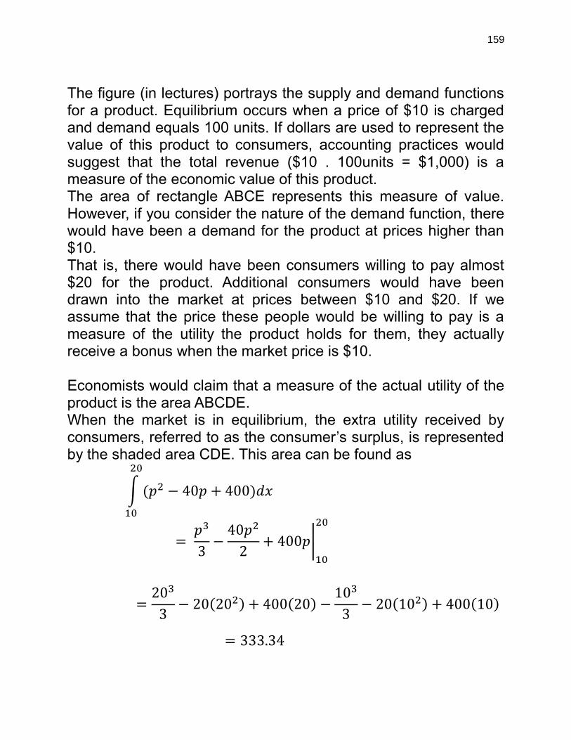
159
The figure (in lectures) portrays the supply and demand functions for a product. Equilibrium occurs when a price of $10 is charged and demand equals 100 units. If dollars are used to represent the value of this product to consumers, accounting practices would suggest that the total revenue ($10 . 100units = $1,000) is a measure of the economic value of this product. The area of rectangle ABCE represents this measure of value. However, if you consider the nature of the demand function, there would have been a demand for the product at prices higher than $10. That is, there would have been consumers willing to pay almost $20 for the product. Additional consumers would have been drawn into the market at prices between $10 and $20. If we assume that the price these people would be willing to pay is a measure of the utility the product holds for them, they actually receive a bonus when the market price is $10. Economists would claim that a measure of the actual utility of the product is the area ABCDE. When the market is in equilibrium, the extra utility received by consumers, referred to as the consumer’s surplus, is represented by the shaded area CDE. This area can be found as
∫ ( − 40 + 400
) 𝑥
=
3−
40
2+ 400 |
=20
3− 20(20 ) + 400(20) −
10
3− 20(10 ) + 400(10)
= 333.34

160
Our accounting methods would value the utility of the product at $1,000. Economists would contend that the actual utility is $1,333.34, or that the consumer’s surplus equals $333.34. This measure of added, or bonus, utility applies particularly to those consumers who would have been willing to pay more than $10.

161
Lecture 31,32
Chapter 20 Optimization: Functions of Several Variables
Partial Derivatives The calculus of bivariate functions is very similar to that of single-variable functions. In this section we will discuss derivatives of bivariate functions and their interpretation.
Derivatives of Bivariate Functions With single-variable functions, the derivative represents the instantaneous rate of change in the dependent variable with respect to a change in the independent variable. For bivariate functions, there are two partial derivatives. These derivatives represent the instantaneous rate of change in the dependent variable with respect to changes in the two independent variables, separately.
Given a function = 𝑓 (𝑥, 𝑦) , a partial derivative can be found with respect to each independent variable. The partial derivative taken with respect to x is denoted by
𝜕𝑧
𝜕𝑥 or 𝑓
The partial derivative taken with respect to y is denoted by
𝜕𝑧
𝜕𝑦 or 𝑓
Although both notational forms are used to denote the partial
derivative, we will use the subscripted notation 𝑓 and 𝑓 .
Partial Derivative Given the function z = f (x, y), the partial derivative of z with respect to x at (x, y) is

162
𝑓 = lim∆
𝑓(𝑥 + ∆𝑥, 𝑦) − 𝑓(𝑥, 𝑦)
∆𝑥
provided the limit exists. The partial derivative of z with respect to y at (x, y) is
𝑓 = lim∆
𝑓(𝑥, 𝑦 + ∆𝑦) − 𝑓(𝑥, 𝑦)
∆𝑥
provide the limit exists. Example
Consider the function 𝑓(𝑥, 𝑦) = 3𝑥 + 5𝑦 . To find the partial derivative with respect to x we consider
𝑓 = lim∆
𝑓(𝑥 + ∆𝑥, 𝑦) − 𝑓(𝑥, 𝑦)
∆𝑥
= lim∆
(3(𝑥 + ∆𝑥) + 5𝑦 ) − (3𝑥 + 5𝑦 )
∆𝑥
= lim∆
(3(𝑥 + ∆𝑥 + 2𝑥∆𝑥) + 5𝑦 ) − (3𝑥 + 5𝑦 )
∆𝑥
= lim∆
(3𝑥 + 3∆𝑥 + 6𝑥∆𝑥 + 5𝑦 ) − (3𝑥 + 5𝑦 )
∆𝑥
= lim∆
3∆𝑥 + 6𝑥∆𝑥
∆𝑥= lim
∆ 3∆𝑥 + 6𝑥 = 6𝑥
Fortunately, partial derivatives are found more easily using the same differentiation rules we used in Chap. 15 – 17. The only exception is that when a partial derivative is found with respect to one independent variable, the other independent variable is assumed to be held constant. For instance, in finding the partial derivative with respect to x, y is assumed to be constant. A very important point is that the variable which is assumed constant must be treated as a constant in applying the rules of differentiation.

163
EXAMPLE
Find the partial derivatives 𝑓 and 𝑓 for the function 𝑓(𝑥, 𝑦) =
5𝑥 + 6𝑦 Solution: The partial derivative with respect to x is
𝑓 = 10𝑥
The partial derivative with respect to y is
𝑓 = 12𝑦.
Example
Find fx and fy for the function 𝑓(𝑥, 𝑦) = 4𝑥𝑦.
Solution: The partial derivative with respect to x is
𝑓 = 4𝑦
The partial derivative with respect to y is
𝑓 = 4𝑥.
Example
Find 𝑓 and 𝑓 for the function 𝑓(𝑥, 𝑦) = 2 2.
Solution: The partial derivative with respect to x is
𝑓 = 2𝑥 2 2
The partial derivative with respect to y is
𝑓 = 2𝑦 2 2.
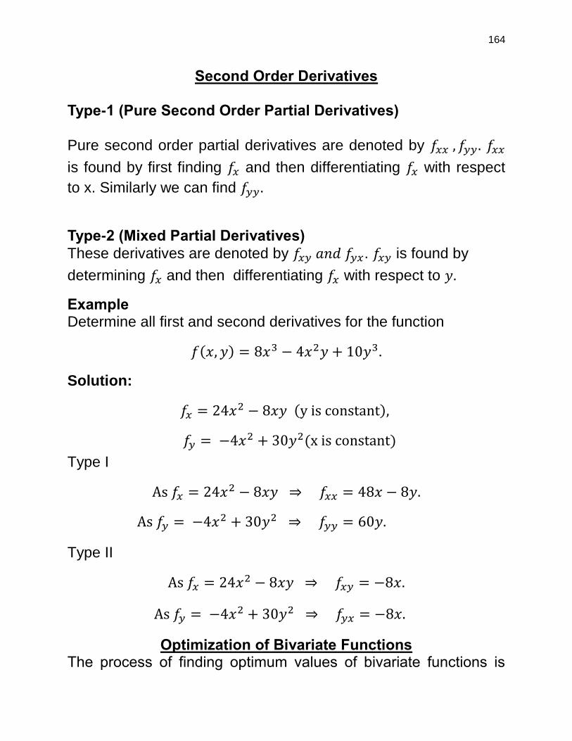
164
Second Order Derivatives Type-1 (Pure Second Order Partial Derivatives)
Pure second order partial derivatives are denoted by 𝑓 , 𝑓 . 𝑓
is found by first finding 𝑓 and then differentiating 𝑓 with respect
to x. Similarly we can find 𝑓 .
Type-2 (Mixed Partial Derivatives)
These derivatives are denoted by 𝑓 𝑎𝑛 𝑓 . 𝑓 is found by
determining 𝑓 and then differentiating 𝑓 with respect to 𝑦.
Example Determine all first and second derivatives for the function
𝑓(𝑥, 𝑦) = 8𝑥 − 4𝑥 𝑦 + 10𝑦 .
Solution:
𝑓 = 24𝑥 − 8𝑥𝑦 (y i on tant),
𝑓 = −4𝑥 + 30𝑦 (x i on tant)
Type I
𝑓 = 24𝑥 − 8𝑥𝑦 𝑓 = 48𝑥 − 8𝑦.
𝑓 = −4𝑥 + 30𝑦 𝑓 = 60𝑦.
Type II
𝑓 = 24𝑥 − 8𝑥𝑦 𝑓 = −8𝑥.
𝑓 = −4𝑥 + 30𝑦 𝑓 = −8𝑥.
Optimization of Bivariate Functions The process of finding optimum values of bivariate functions is
165
very similar to that used for single variable functions. As with single-variable functions, we will have a particular interest in identifying relative maximum and minimum points on the surface representing a function f(x,y). Relative maximum and minimum points have the same meaning in three dimensions as in two dimensions. Relative Maximum A function z = f (x, y) is said to have a relative maximum at x = a and y = b if for all points (x, y) “sufficiently close” to (a, b)
f (a, b) ≥ f (x, y) Relative Minimum A function z = f (x, y) is said to have a relative minimum at x = a and y = b if for all points (x, y) “sufficiently close” (a, b)
f (a, b) ≤ f (x, y) Necessary Condition For Relative Extrema A necessary condition for the existence of a relative maximum or a relative minimum of a function f whose partial derivatives fx and fy both exist is that:
𝑓 = 0 and 𝑓 = 0
Critical Points The values x* and y* at which fx = 0 and fy = 0 are critical values.
The corresponding point (x*, y*, f (x*, y*)) is a candidate for a
relative maximum or minimum on f and is called a critical point.
Example Locate any critical points of the function
𝑓(𝑥, 𝑦) = 4𝑥 − 12𝑥 + 𝑦 + 2𝑦 − 10.

166
Solution: Since 𝑓 = 8𝑥 − 12, and 𝑓 = 2𝑦 + 2. For critical points
we set 𝑓 = 0 and 𝑓 = 0.
𝑓 = 0 8𝑥 − 12 = 0 𝑥 =3
2
𝑓 = 0 2𝑦 + 2 = 0 𝑦 = −1
Now
𝑓 (3
2, −1) = 4 (
3
2)
− 12 (3
2) + (−1) + 2(−1) − 10 = −20
The only critical point is (
, −1,−20).
Distinguishing Nature of Critical Points Once a critical point has been identified, it is necessary to determine its nature. Aside from relative maximum and minimum points, there is one other situation in which fx and fy both equal 0, which is referred to as a saddle point. A saddle point p is a portion of a surface which has the shape of a saddle , at point “where you sit on the horse” the value of fx and fy both equal 0. However, the function does not reach either a relative maximum or a relative minimum at p. Test of Critical Point
Given that a critical point of 𝑓 is located at (𝑥 , 𝑦 , 𝑧) where all second partial derivatives are continuous, determine the value of
D (𝑥 , 𝑦 , 𝑧), where
𝐷 (𝑥 , 𝑦 ) = |𝑓 𝑓
𝑓 𝑓 | = f (𝑥
, 𝑦 )f (𝑥 , 𝑦 ) − [𝑓 (𝑥 , 𝑦 )]
I- If 𝐷(𝑥 , 𝑦 ) > 0, the critical point is
a) A relative maximum if both 𝑓 (𝑥 , 𝑦 ) and 𝑓 (𝑥 , 𝑦 ) are
negative.

167
b) A relative minimum if both 𝑓 (𝑥 , 𝑦 ) and 𝑓 (𝑥 , 𝑦 ) are
positive.
II- If 𝐷(𝑥 , 𝑦 ) < 0, the critical point is a saddle point.
III- If 𝐷(𝑥 , 𝑦 ) = 0, no conclusion can be drawn.
Example
Given the function 𝑓(𝑥, 𝑦) = −𝑥 − 𝑦 + 12𝑦 . Determine the location and nature of the critical points. Solution: Here
𝑓 = −2𝑥, 𝑓 = 3𝑦(8 − 𝑦)
Put 𝑓 = 0 which gives us 𝑥 = 0, and for 𝑓 = 0 gives us
3𝑦(8 − 𝑦) = 0 𝑦 = 0, 8.
Thus we have two critical points (0, 0, 0) and (0,8, 256). Second
order derivatives are
𝑓 = −2, 𝑓 = 0 = 𝑓 and 𝑓 = −6𝑦 + 24.
Taking (0, 0, 0)
𝐷(0, 0) = (−2)(24) − 0 = −48 < 0
This implies a Saddle point occurs at (0, 0, 0).
Taking (0, 0, 0)
𝐷(0, 0) = (−2)(−48 + 24) − 0 = 48 > 0
This implies a critical point is either relative maximum or
minimum. As 𝑓 < 0 and 𝑓 < 0, we conclude that relative
maximum occurs on 𝑓 at (0, 8, 256).

168
Applications of Bivariate Optimization This section presents some applications of the optimization of bivariate functions. Example (Advertising Expenditures) A manufacturer’s estimated annual sales (in units) to is a function
of the expenditures made for radio and TV advertising. The
function specifying this relationship was stated as
𝑧 = 50000 𝑥 + 40000𝑦 − 10𝑥 − 20𝑦 − 10𝑥𝑦
where z equals the number of units sold each year, x equals the
amount spent for TV advertising and y equals the amount spent
for radio advertising (x and y both in $1,000s). Determine how
much money should be spent on TV and radio advertising in order
to sell maximum number of units.
Solution:
Here 𝑓 = 50000 − 20𝑥 − 10𝑦 and 𝑓 = 40000 − 40𝑦 − 10𝑥. Put
𝑓 = 0 and 𝑓 = 0 we obtain
20𝑥 + 10𝑦 = 50000
10𝑥 + 40𝑦 = 40000
Solving simultaneously we get 𝑥 = 2285.72 and 𝑦 = 428.57. Now
taking double derivative we have 𝑓 = −20, 𝑓 = −10, 𝑓 =
−10 and 𝑓 = −40.
Testing critical point
𝐷(2285.72, 428.57) = (−20)(−40) − (−10) = 700 > 0
Since 𝐷 > 0, both 𝑓 , 𝑓 are negative, hence annual sales are
maximum at

169
𝑓(𝑥, 𝑦) = 𝑓(2285.72, 428.57) = 65714296 unit .
Example (Pricing Model) A manufacturer sells two related products, the demands for which
are estimated by the following two demand functions:
= 150 − 2 −
= 200 − − 3
where pj equals the price (in dollars) of product j and qj equals the
demand (in thousands of units) for product j. Examination of these
demand functions indicates that the two products are related. The
demand for one product depends not only on the price charged
for the product itself but also on the price charged for the other
product. The firm wants to determine the price it should charge for
each product in order to maximize total revenue from the sale of
the two products.
Solution: This revenue-maximizing problem is exactly like the single-product problems discussed in Chap. 17. The only difference is that there are two products and two pricing decisions to be made. Total revenue from selling the two products is determined by the function
= +
This function is stated in terms of four independent variables. As
with the single-product problems, we can substitute the right side
of equations
We can now proceed to examine the revenue surface for relative
maximum points.
1 1 2 2 1 2
2 2
1 1 1 2 2
2 2
1 1 1 2 2 2
(150 2 ) (200 3 )
150 2 3
150 2 2 200 3
R p p p p p p
p p p p p
p p p p p p

170
The first partial derivatives are
𝑓 1= 150 − 4 − 2 , 𝑓 2
= −2 + 200 − 6
𝑓 1= 0 4 + 2 = 150 𝑎𝑛 𝑓 2
= 0 2 + 6 = 200
Solving simultaneously the above two equations we obtain
= 25, = 25.
Testing for critical points
𝑓 1 1= −4, 𝑓 1 2
= −2 = 𝑓 2 1, 𝑓 2 2 −
Therefore 𝐷(25,25) = 20 > 0. As 𝑓 1 1, 𝑓 2 2
both are negative
relative maximum occurs at = = 25.
Revenue will be maximized at a value of 𝑓(25,25) = $ 4,375
(thousands) when each product is sold for $25. Expected demand
at these prices can be determined by substituting and into
the demand equations, or
= 150 − 2(25) − 25 = 75(Thousand units)
= 200 − 25 − 3(25) = 100(Thousand units)
Example (Satellite Clinic Location) A large health maintenance organization (HMO) is planning to
locate a satellite clinic in a location which is convenient to three
suburban townships. The HMO wants to select a preliminary site
by using the following criterion: Determine the location (x, y)
which minimize the sum of the squares of the distances from each
township to the satellite clinic.
Solution: The unknown in this problem are x and y, the coordinates of the satellite clinic location.

171
We need to determine an expression for the square of the distance separating the clinic and each of the towns. Given the
point (𝑥 , 𝑦 ) and (𝑥 , 𝑦 ), the distance formula gives
= √(𝑥 − 𝑥 ) + (𝑦 − 𝑦 )
We obtain
= 3𝑥 + 3𝑦 + 60𝑥 − 40𝑦 + 2700
Taking derivatives
𝑓 = 6𝑥 − 60, 𝑓 = 6𝑦 − 40.
Now we put 𝑓 = 0 = 𝑓 which gives us
𝑥 = 10, 𝑦 =20
3.
Critical point testing
𝑓 = 6, 𝑓 = 6, 𝑓 = 𝑓 = 0
𝐷 (10,20
3) = 36 > 0
Relative minimum occurs when 𝑥 = 10, 𝑦 =
.
2 2 2 2
2 2
( , )
[( 40) ( 20) ] [( 10) ( 10) ]
[( 20) ( 10) ]
S f x y
x y x y
x y