1

Landslide susceptibility by mathematical model in Sarno 1

area. 2

3

G. Capparelli1, P. Versace1, 4

[1] Department of Environmental and Chemical Engineering, University of Calabria - 5

Arcavacata di Rende (CS) - Italy 6

Correspondence to: G. Capparelli (giovanna.capparelli@unical.it) 7

8

Abstract 9

Rainfall is recognized as a major precursor for many types of slope movements. Technical 10

literature reports many examples both of study cases and models related to landslides induced 11

by rainfall. Subsurface hydrology has a dominant role since changes in the soil water content 12

affect significantly the soil shear strength. The analytical approaches are very different, 13

ranging from statistical models to distributed models and complete, these last ones able to 14

take several components into account, including specific site conditions, mechanical, 15

hydraulic and physical soil properties, local seepage conditions, and the contribution of these 16

to soil strength. The paper reports a study carried out by using a complete model, named 17

SUSHI (Saturated Unsaturated Simulation for Hillslope Instability), on a case of great interest 18

both for the complexity of the phenomenon and the severity with which it occurred. 19

The landslide-prone area is located in Campania region (Southern Italy), were disastrous 20

mud-flows occurred in May 1998. The region has long been affected by rainfall-induced slope 21

instabilities that often involved large areas, causing many victims. The applications allowed 22

understanding better the role of the rainfall infiltration and of the suction changes in the 23

triggering mechanism of the phenomena. These changes must be carefully considered when 24

dealing with slope stability conditions for assessing hazard conditions and planning 25

engineering works. 26

27

28

2

1 Introduction 1

The problems and the damages caused by landslides become complex and worrisome, 2

accounting each year for huge property damage in terms of both direct and indirect costs. 3

Social and economic losses due to landslides can be reduced by means of effective planning 4

and management. The approaches include actions like the limitation of development in 5

landslide-prone areas, the use of appropriate construction rules, the use of physical measures 6

to prevent or control landslides and the setting up early warning systems. To address solutions 7

to the landslide problem, it is necessary to develop a better understanding of landslide hazard 8

regard the trigger mechanisms, propagation and impact structures. 9

Landslides can be attributed to a number of factors, such as geologic features, topography, 10

vegetation, weather, or their combinations. Among the factors which contribute to the 11

occurrence of these phenomena, rainfall is one of the most important. 12

As a result of rainfall events and subsequent infiltration into the subsoil, the soil moisture can 13

be significantly changed with a decrease in matric suction in unsaturated soil layers and/or 14

increase in pore-water pressure in saturated layers. As a consequence, in these cases, the shear 15

strength can be reduced enough to trigger the failure. 16

The occurrence of the phenomena is also influenced by heterogeneity of hydraulic and 17

geotechnical properties and water interaction. The complex hydrological responses of natural 18

slopes are strongly influenced by the infiltration into unsaturated soil, generation of surface 19

runoff, slope-parallel flow of a perched groundwater table, subsurface flow from upstream 20

area, effect of vegetation, flow through macropores and discontinuities and into fractured 21

bedrock. All these issues affect the predictive ability of the simulation models and, 22

sometimes, the comprehension of the phenomena they can provide. 23

In addition, the shear strength contribution from soil suction above the groundwater table is 24

usually ignored if the major portion of the slip surface is below the groundwater table. But 25

negative pore water pressures can no longer be ignored in situations characterized by deep 26

ground water table and shallow failure surface (Lu and Godt, 2013). 27

Technical literature reports many analytical approaches that differ for: the spatial scale range 28

adopted that varies from wide area, up to ten of thousands kilometers, to small area, that can 29

be reduced to a single landslide; the quality and quantity of hydrologic, hydraulic and 30

3

geotechnical available data; the adopted detail for describing the hydrological and 1

geotechnical mechanisms in slope. 2

Very popular models are the hydrological models that directly analyze the rainfall identifying 3

the threshold values. These values are assumed on the basis of historical available data, are 4

drawn in the intensity-duration plot as proposed by Caine (1980) and provide lower limit of 5

rainfall associated to the occurrence of landslides, shallow landslides and debris flows 6

(Guzzetti, 2008). 7

Other types of rainfall thresholds (Glade, 2000; Rahardjo et al., 2001) consider the effect of 8

the antecedent rainfall precipitation more important than the rainfall recorded on the day of 9

landslide occurrence. Usually this type of approach is related to the study of more complex 10

landslides. The influence of antecedent rainfall on the slope stability is a topic of discussion 11

(Martelloni et al., 2011). 12

These models are an important tool to support the prediction of landslides, applicable for 13

early warning system (Capparelli & Tiranti 2010) and over wide areas. However, they don’t 14

provide any information about the hydrological processes involved in a landslide area and 15

don’t improve our understanding of landslide dynamics. 16

On the contrary, complete models can help in understanding triggering mechanisms since 17

they attempt to reproduce the physical behavior of the processes involved at hillslope scale, 18

employing detailed hydrological, hydraulic and geotechnical information (Montgomery and 19

Dietrich, 1994; Pack et al., 1998; Rigon et al, 2006;Tsai et al., 2008). 20

These models develop analysis over wide areas and usually produce a susceptibility map 21

characterizing the landslide prone zones according to a stability index. They are generally 22

composed by an hydrological and geotechnical module. While the computation of the safety 23

factor, in most cases, is performed by the limit equilibrium method, under the assumption of 24

infinite slope, the hydrological modules present substantial differences. 25

The approach proposed in Shalstab (Montgomery and Dietrich, 1994) supposes a constant 26

infiltration rate, neglects soil moisture above the water table, does not take into account the 27

transient response to rainfall and considers the groundwater flows parallel to the slope. The 28

assumptions are too restrictive, for example, when pore water pressure responds very quickly 29

to transient rainfall and its redistribution has a large component normal to slope. 30

4

Wu and Sidle (1995) combined also the infinite slope equation with a subsurface flow model 1

based on the kinematic wave approximation, taking also into account the vegetation root 2

strength. An enhanced version of this model is proposed by Dhakal and Sidle (2004) that 3

investigate the influence of different rainfall characteristics on slope stability. 4

Iverson (2000) developed a flexible modeling framework by modeling a one-dimensional 5

linear diffusion process in saturated soil and using an analytical solution of the Richards 6

equation. The model is valid for hydrological modeling in nearly saturated soil. According to 7

this hypothesis, established to find an analytical solution of pressure heads, the infiltration 8

capacity is assumed to be equivalent to the saturated hydraulic conductivity, instead of 9

considering it as variable with time during the rainfall event. Furthermore, the Author 10

considers ground surface of hillslope subject to a uniform rainfall. 11

For taking into account the variability of rainfall intensity and duration, dynamic or quasi-12

dynamic models have been introduced (Baum et al. 2002). The model, TRIGRS 1.0, allows a 13

more precise description of slope hydrology but requires a large number of parameters. 14

Recently, TRIGRS 2.0 (Baum et al., 2010) allows calculating the filtration process in 15

unsaturated soils coupled with a diffusive propagation in saturated soils. 16

The scheme proposed by Iverson has been adopted in D’odorico et al (2005) to investigate the 17

effect of hyetograph characteristics on landslide potential. 18

For taking into account of hydrological phenomena Arnone et al. (2011) proposed the tRIBS 19

model (Triangulated Irregular Network Real-Time Integrated Basin Simulator) that allows 20

simulation of most of spatial-temporal hydrologic processes (infiltration, evapotranspiration, 21

groundwater dynamics and soil moisture conditions) that can influence landsliding. 22

Most of the aforementioned approaches rely on the restrictive assumption of a steady-state 23

subsurface flow, which can affect the predictive capability of the models both in terms of 24

accuracy and timing of the prediction. Any model must always be validated regardless the 25

implemented schemes by checking, for example, the accuracy of the simulation with the 26

available experimental data or real case. The results can sometimes be very different applying 27

different models to the same event, how described in Sorbino et al (2010) that illustrate how 28

applying three different physically based models (SHALSTAB, TRIGRS and TRIGRS-29

unsaturated) on the same set of geo-environmental cases different results were obtained. The 30

results reveal the advantages and limitations of each model in landslide forecasting. 31

5

For sure, these types of spatial distributed modeling are well-suited for shallow landslides but 1

in larger landslides their efficiency is decreased by the higher complexity of the phenomena 2

(van Westen et al.2003). 3

A detailed analysis of the individual mechanisms which occur in favor of landslide triggering 4

is required for proper investigation by using complete models that can reproduce the spatial 5

and temporal pattern of water flows in very well detailed domains. 6

In this work the complete model named SUSHI, Simulation for Saturated Unsaturated 7

Hillslope Instability, (Capparelli and Versace, 2011) is applied in a very complex case to 8

improve the understanding of the slope failure mechanism during rainfall infiltration. 9

SUSHI model takes into account several components, as specific site conditions, mechanical, 10

hydraulic and physical soil properties, locale seepage conditions and their contribution to soil 11

strength. 12

It is composed by a hydraulic module, to analyse the subsoil water circulation due to the 13

rainfall infiltration under transient conditions and by a geotechnical module, which provides 14

indications regarding the slope stability starting from limited equilibrium methods. 15

The hydraulic process is illustrated by the implementation of finite difference procedure that 16

solves Richard’s equation which is used to represent saturated/unsaturated flow within a 17

hillslope. The temporal and spatial distribution of moisture content in subsurface are 18

performed in order to evaluate different contribution as downslope and vertical components 19

in flow regime in hillslope by unsteady rainfall. 20

Furthermore, the model was developed in order to be suitable for cases with strongly 21

heterogeneous soils, irregular domains and boundary conditions variable in space and time. 22

After a brief description of the model, the paper describes the analysis and the representative 23

results obtained for the volcaniclastic covers of Sarno (Campania region - Southern Italy), 24

where dangerous mud flows occurred in May 1998. 25

26

2 SUSHI model framework 27

The model is based on the combined use of two modules: HydroSUSHI, aimed at studying 28

subsoil water circulation and GeoSUSHI, suited for evaluating the degree of slope stability. 29

Infiltration analysis is carried out by using Richards’ equation (1931), expressed as pressure-30

6

based methods to enable applications for layered soils and transient flow regime for both 1

saturated and unsaturated conditions. 2

HydroSUSHI analyses subsoil water circulation in a spatial 2D domain which can be 3

characterized by irregular soil stratigraphy with different hydrogeological properties. 4

By adopting a Cartesian orthogonal reference system Oxz, with z-axis positive downwards, 5

the governing differential equation is: 6

t

SSCzK se

(1) 7

where TLK / is the hydraulic conductivity which depends on pressure head L for 8

unsaturated soils (ignoring soil anisotropy). The formula on the right was modified to 9

simulate water flow in both unsaturated and saturated zones, so avoiding the use of different 10

algorithms for the resolution of parabolic and elliptic equations respectively (Paniconi et al., 11

1991). /C [L-1] is specific soil water capacity in the unsaturated zone, which 12

represents the rate at which a soil absorbs or releases water when there is a change in pressure 13

head; 1LSS is the specific volumetric storage. Effective Saturation rsreS / , 14

where is the water content, s is the porosity and r is the residual water content, can be 15

computed using the Soil Water Retention Curve (van Genuchten and Nielsen, 1985). The 16

saturated flow equation is simply a special case of Richards’s equation in which the 17

conductivity and storage terms are not functions of pressure head. 18

Recently, this module was upgraded through the integration of a method for the 19

evapotranspiration process description, even if this component usually produces secondary 20

effects when slope mobilizations occur in very rainy periods (Capparelli and Versace 2011). 21

Since the study case proposed in the paper develops into a winter season, the effects related to 22

evapotranspiration were neglected, because totally irrelevant in understanding the dynamics 23

occurred. 24

Richards’ equation does not allow analytical solutions unless in cases where simplifying 25

hypotheses and /or particular boundary conditions are introduced, (Iverson, 2000; Srivastava e 26

Yeh,1991). In HydroSUSHI module the finite differences (FDM) scheme and the fully 27

implicit method are adopted. 28

7

Examples of finite difference algorithms which deal either variably saturated or fully 1

unsaturated conditions are proposed by Freeze (1978) and Vauclin et al. (1979). The finite-2

difference method is one of the oldest numerical methods known for solving partial 3

differential equations (pde). In this approach, the continuous problem domain is discretized so 4

that the dependent variables are considered to exist only at discrete points. 5

Figure 1 draws an example of spatial discretization which is composed by regular mesh 6

zx ; . The size to be assigned to zx ; should be suitably selected depending on the 7

complexity of the stratigraphy. It is important, in fact, to ensure a faithful reproduction of the 8

layers, so as to guarantee a realistic representation of water flow exchanges. 9

With reference to the generic node with coordinates xixx 0 , zjzz 0 according to 10

the finite difference scheme, the equation 1, can be written as: 11

tC

xK

zK

z

xK

xK

x

kji

kjik

jiSU

kji

kjik

ji

kji

kjik

ji

kji

kjik

ji

kji

kjik

ji

,1

,1,

11,

1,)1(

2/1,

1,

11,)1(

2/1,

1,1

1,)1

,2/1

1,

1,1)1

,2/1

111

1

(2)

12

where seSU SSCC , the subscripts ji ,2/1 and 2/1, ji indicate quantities 13

evaluated at the spatial coordinates zjzxix 00 ,2/1 , and 14

zjzxix 2/1, 00 , t is the time step, the superscripts )(k and )1( k indicate 15

quantities referring to time instants tktt 0 and tktt 10 . 16

To solve the equation (1) boundary conditions along the edges of the domain problem must be 17

specified. A general form of the boundary conditions for this pde can be written (McCord, 18

1991): 19

tBn G

,

(3)

20

where , and tB , are given functions evaluated on the boundary region G , the 21

expression n / is normal derivative operator and it spatial local vector. 22

8

By applying this general formulation for water flow modelling the conditions become (figure 1

1): along the basal impermeable boundary BC and vertical boundary AB a Neumann 2

condition in considered, whit flux equal to zero , then K ,0 and 3

0,, tqtB . In terms of total hydraulic head zh : 4

0

BCz

h (3.1) 5

0

ABx

h (3.2) 6

For vertical down-slope side DC we take into account the influence of the increasing 7

subsurface flow, by considering both situations of unsaturated and saturated layers. This is 8

computed by adopting boundary conditions moving from Neumann to Dirichlet condition, 9

with specified flux or pressure head respectively, 0,1 and thtB ,, . 10

Then: 11

0,

txqx

h

DC

(3.3) 12

0DC

(3.4) 13

On the upper boundary AD we allow a time-dependent rainfall TLr / . The boundary 14

condition can be stated by considering the infiltration rate txI , as: 15

ADz

txhtxKtxI

,

,, (3.5) 16

In particular: 17

z

txhtxKtxrif

z

txhtxKtxI

z

txhtxKtxriftxrtxI

,,,

,,,

,,,,,

(3.5a) 18

The value txK , will depend on the values of tx, at the point x at time t and on the 19

nature of the K curve for the surface soil at x . 20

21

9

Validation tests were carried out by the comparison of HydroSUSHI outputs with 1

experimental solutions proposed in Vauclin et al. (1979), in Paniconi & Putti (1994) and with 2

the suction data collected by the jet fill tensiometers located in a pilote site (Capparelli and 3

Versace, 2011). The comparison of results for both applications was satisfactory and 4

confirmed the capability of the model to simulate groundwater circulation. 5

Concerning GeoSUSHI module, stability analysis is performed for better understanding of the 6

role of negative pore-water pressures (or matric suction) in increasing the shear strength of the 7

soil. 8

It may be a reasonable assumption to ignore negative pore-water pressures for many 9

situations where the major portion of the slip surface is below the groundwater table. 10

However, for situations where the groundwater table is deep or where concern is over the 11

possibility of shallow failure surface, negative pore-water pressures can no longer be ignored. 12

Recently Lu and Godt (2013) present an interesting work on understanding and quantifying 13

the hydro-mechanical processes for predicting the spatial and temporal occurrence of 14

landslide. The Authors provide quantitative treatments of rainfall infiltration, effective stress, 15

their coupling and roles in hillslope stability, by introducing a unified effective stress 16

framework linking soil suction to effective stress. 17

The procedure here proposed is an extension of conventional limit equilibrium methods 18

adapted for the unsaturated soils as suggested by Fredlund and Rahardjo (1993). 19

The shear strength of an unsaturated soil can be formulated in terms of independent stress 20

state variables au and wa uu as follows: 21

bfwafanff uuuc tan'tan' (4) 22

where the subscripts f indicate quantities evaluated at on the failure plane at failure, the ff 23

is shear stress, 'c is effective cohesion, fan u net normal stress state, au pore-air 24

pressure, ' effective friction angle, wa uu matric suction, b angle indicating rate of 25

increase in shear strength relative to the matric suction. In practical applications, this last term 26

is evaluated using the expression proposed by Vanapalli et al. (1996). The equation (4) is an 27

extension of shear strength equation for a saturated soil. As the soil approaches saturation, the 28

pore-water pressure, wu , approaches the pore-air pressure au and matric suction wa uu 29

10

goes to zero. The General Limit Equilibrium method (i.e GLE) provides a general theory 1

wherein other methods can be viewed as special cases. It’s well known, the elements used in 2

GLE method for deriving the safety factor (FS) are the summation of forces in two directions 3

and of the moments about a common point (Fredlund and Rahardjo;1993).Calculations for the 4

stability of a slope are performed by dividing the soil mass above the slip surface into vertical 5

slices. The mobilized shear force at the base of a slice can be written using the shear strength 6

for an unsaturated soil: 7

bwaanm uuuc

FSS

tan'tan' (5) 8

where mS is the shear force mobilized on the base of the slice; sloping distance across the 9

base of a slice; FS safety factor which defined as the factor by which the shear strength 10

parameters must be reduced in order to bring the soil mass into a state of limiting equilibrium 11

along the assumed slip surface. 12

13

3 General description of the investigated context. 14

The case study proposed in the paper is located in Campania region (Southern Italy), where 15

catastrophic flowslides and debris flows in pyroclastic soils are very usual. A brief list of 16

some recent events is reported in Table 1 which includes also information about the size of 17

the landslide. 18

Pizzo d’Alvano is a NW-SE oriented morphological structure, consisting of a sequence of 19

limestone, dolomitic limestone and, subordinately, marly limestone dating from the Lower to 20

Upper Cretaceous age. The slopes are mantled by very loose pyroclastic soils that are the 21

result of explosive activity of the Somma-Vesuvius volcanic, both as primary air-fall deposits 22

and volcanoclastic deposits, according to the mode of transport and deposition (Rolandi, 23

1997). 24

Air-fail deposits were dispersed from N-NE to S-SE, according to prevailing wind direction 25

and covered a wide area reaching distances up to 50 km. Pumiceous and ashy deposits 26

belonging to at least 5 different eruptions were recognized. From the oldest to the youngest, 27

they are: Ottaviano (8000 years b.p.; E-NE dispersion direction), Avellino (3800 years b.p.; 28

E-NE dispersion direction), 79 A.D. (E-SE dispersion direction), 472 A.D. (N-NE dispersion 29

direction), 1631 A.D. (N-NE dispersion direction). The deposits are affected by pedogenetic 30

11

processes determining paleosoil horizons during rest phases of the volcanic activity. The total 1

thickness of the pyroclastic covers in these areas ranges between few decimetres to 10 meters, 2

near to the uppermost flat areas. The general structure of the soil progressively adapts itself to 3

the morphology of the calcareous substratum showing, therefore, complex and variable 4

geometries (Rolandi,1997) 5

3.1 Shallow landslide events and main interpretations 6

On May 5, 1998, a huge number of mud flows were triggered on the slopes of the Pizzo 7

d’Alvano massif, (Figure 2) involving an extension area of around 60 Km2, a volume of 8

2.000.000 m3 (40% derived from the eroded materials along the channels) and causing 165 9

victims and huge damages to urban centres Sarno, Quindici, Siano and Bracigliano. 10

These landslides were classified as very rapid to extremely rapid soil slip/debris flows (Ellen 11

e Fleming, 1987) that travelled down-slope and then propagated in highly urbanized areas. 12

A characteristic element is the run-out distances that ranged from a few hundred meters up to 13

distances greater than 2 km (Revellino et al.,2004) and speeds that, at the toe of channels, 14

were estimated to be in the range of about 5–20 m/s. 15

Many similar phenomena have afflicted various other parts of the world, (Japan in 1985, the 16

west coast of United States – California (1973, 1982, 2005), Brazil (1967), Venezuela (1999) 17

sometimes involving similar pyroclastic soils. Even in Italy, as the disastrous mudslide with a 18

volume of 180.000 m3 which completely destroyed the Val di Stava village (it was July 19, 19

1985), due to the failure of two settling basins for industrial use, which caused the death of 20

268 people . 21

Although the triggering mechanism are different and sometimes the involved soils are not 22

always similar, the common feature seems to be the presence of particles with a high porosity 23

and a very low degree of cementation, which have a sudden change due to the action of an 24

external agent (such as an earthquake or more often a rainfall event) which produces a rapid 25

increase in pore water pressure. 26

A singularity of the landslides occurred in May 1998, which made the events even more 27

tragic, is represented by their simultaneity; the distribution in time and space, the volume of 28

material, take an unusual connotation. These phenomena are particularly dangerous and 29

destructive due to the lack of clear warning signs, the high capacity erosive. 30

12

They were analyzed in several papers that indicate the most significant geomorphological, 1

hydrological and geotechnical features of the involved slopes and models for the triggering 2

mechanisms and propagation of landslides. 3

Cascini et al (2008) argue that the instabilities in Sarno was caused by a combined effect of 4

water infiltrated in the surface layers and the one coming from the bedrock in correspondence 5

to a temporary spring. This assumption was introduced considering, in the following years, 6

springs from the bedrock were recorded during spring season. The main hypothesis is that the 7

rainfall recorded in the hours immediately before the landslide events, has contributed to 8

change the surface soil water circulation, in a slope already at limit of the equilibrium. 9

Calcaterra et al (2000) discuss the role played by grandwater circulation inside both the 10

pyroclstic deposits and the karst cavities of the underlying limestone bedrock. 11

Even before the events of 1998, other Authors (Celico et al 1986) analyzing some events that 12

occurred in pyroclastic covers in Campania region, have considered important not so much 13

the previous daily rainfall as its relationship with the accumulated rainfall in the days or 14

weeks before the landslide events. 15

The importance of soil water circulation is relevant due to the typical stratification pyroclastic 16

covers, where one or more layers of pumice, with high permeability and layers of paleosoils, 17

with lower permeability, are present. This situation encourages, when persistent rainfall 18

events occur, runoff sub-surface conditions that may predispose to the slope instability in 19

limited area. There is also discussion between who supports the importance of vegetation and 20

plant roots and analyzes the possible relations with the instability (Mazzoleni et al, 1998). 21

They emphasize the highly dynamic nature of the whole soil-vegetation, in which the 22

hydrological processes can vary greatly as a result of the dynamics of vegetation. Abrupt 23

changes in vegetation cover can produce equally rapid effects on soil and water regime. 24

Other authors, however, emphasize the role of the suction levels both to explain the trigger 25

mechanisms and the condition that guarantees the stability in high slope (Greco et al., 2013). 26

Among the reasons, many authors have emphasized the importance of liquefaction with the 27

sudden change of the soil, a structure initially characterized by a solid skeleton with a flow 28

characterized by a fluid-like behavior ( Olivares and Picarelli 2003). 29

13

3.2 In-situ conditions and information about rainfall triggering event 1

In the years following the landslide events, many filed surveys have been carried out in these 2

areas, in order to assess the nature of the soil, the hydraulic and geotechnical characteristics. 3

For assessing the influence in the triggering mechanism, suction measurements were also 4

performed along the Tuostolo basin (Sarno area), very close to areas collapsed in May 98 5

(Cascini e Sorbino, 2004), using “Quick-Draw” portable tensiometers and “Jetfill” in-place 6

tensiometers. 7

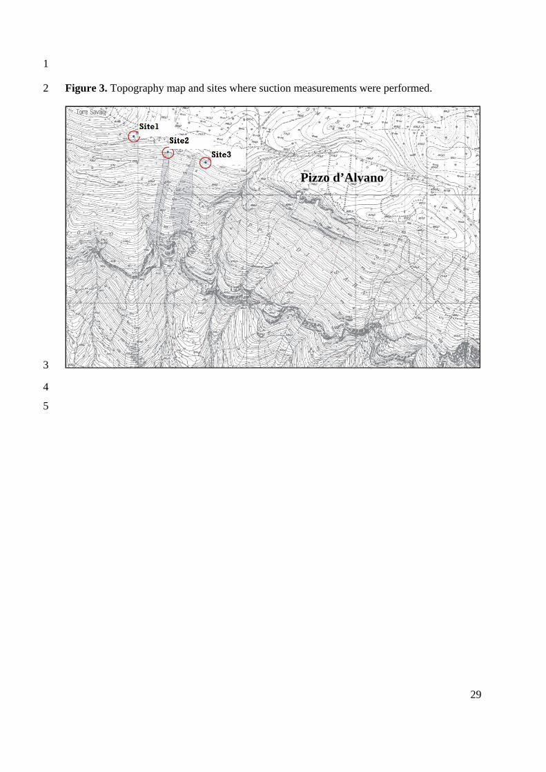
These measurements were taken at three sites (Figure 3), at different depths from the ground 8

surface. In particular, site n.1 was located in an area not affected by the landslides in 1998; 9

sites 2 and 3 in landslide source areas. A significant data scattering can be noted (Figure 4), 10

essentially related to the differences among the sites, the depths at which the measurements 11

were carried out, and also to the local factors that induce changes at the end of the dry season 12

when the acquired data show suction levels very high (around 65 kPa). The data also confirm 13

a high sensitivity of the safety factor regarding the values of the cohesion instead of change in 14

friction angle. The pyroclastic deposits covering the affected areas rest on slopes with high 15

slope angles greater than 40 ° and also have thicknesses ranging from a few centimetres to 16

few meters. In such geomorphological conditions, the soil suction, which increases the shear 17

strength, is a major contributor to the stability, especially at slopes higher than the friction 18

angle of the involved soils. The in-situ investigations show how the pyroclastic covers have 19

friction angles between 32° and 38° and effective cohesion ranging from 0, pumice not 20

reworked, to 4 -5 kPa for the ashy layers. These considerations justify the interest for the 21

suction assessment in these pyroclastic soils as a major predisposing cause, if not the largest. 22

The availability of models able to simulate the circulation of water in these complex terrains 23

can provide useful tool for better understanding these phenomena. 24

The rainfall data was recorded by Sarno - Santa Maria La Foce rain gauge, located at 192m 25

a.s.l , lower than the landslide source areas ,700m a.s.l. 26

The rainfall event, occurred on May 1998, has not been significant, revealing return period 27

less than 5 years, but the period when it occurred makes it remarkable. 28

In fact, the monthly values of April and May in 1998 are significantly higher than the mean 29

rainfall and the maximum daily rainfall values over 1967-1997 (Table 2). Also, on May 98, 30

the rainfall has been recorded mostly in the first six days, with a total 114.6 mm. (Figure 5). 31

14

4 Sushi model application 1

Sushi model described was applied to the mudflow occurred in Tuostolo basin, highlighted by 2

the red square in Figure 2, which destroyed Sarno village. 3

The actual geometry of the mudflow is the result of the coalescence of more landslides 4

succeeded over a period of 6-8 hours. 5

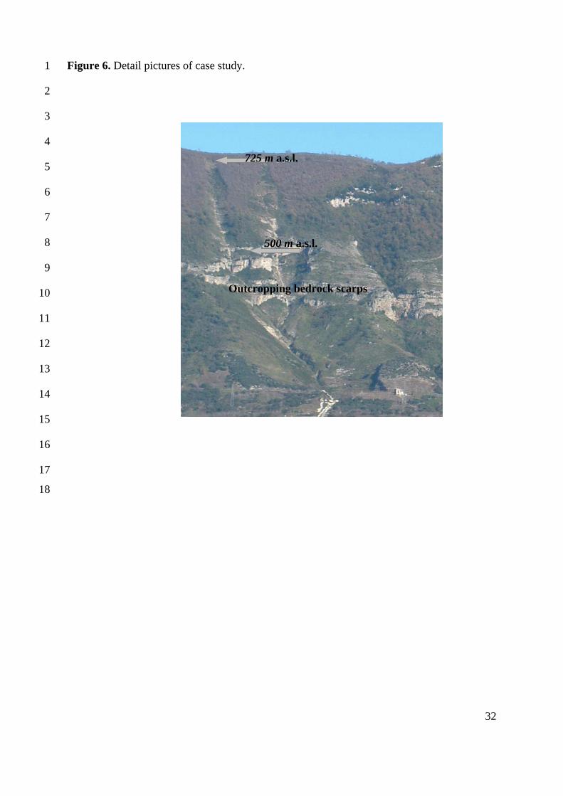
The landslide has mobilized a volume of about 92,000 m3 of volcaniclastic materials resting 6

over carbonate bedrock, including the eroded material within the channel. It developed, from 7

an altitude of about 725 m, to the morphological frame, represented by sub-vertical limestone 8

wall which is situated at an altitude of about 500 m (Figure 6). 9

Most of the landslide occurred on May '98, started just in correspondence of discontinuity 10

morphological, also represented by topographic variations or anthropogenic discontinuity 11

such as roads. 12

The application was developed with the aim of establishing an interpretative model of the 13

triggering phase of the mudflow and its relations with the infiltration of rainwater in the 14

pyroclastic covers. 15

4.1 Input data and slope scheme 16

To define the dynamics of the water circulation in the subsoil, the solution process requires 17

the description of the investigated domain, the soil water characteristic curves, the 18

permeability functions, the mechanical properties of the involved soils, the boundary and 19

initial conditions. 20

Surveys and studies carried out by using also information available in the literature indicated 21

the presence of alternating layers of pumice with a composition and thickness related to the 22

characteristics of the eruptions and to the distance from the eruptive centres. 23

This sequence comprises both primary air-fall and volcanoclastic deposits. The primary 24

deposits are composed by alternating layers of pumice, with interbedded paleosoils. At the 25

basis of this sequence, above the bedrock, there is a layer of red-dark clayey ashy soil 26

(“regolite”) with rare limestone fragments. 27

By using the available topographic maps showing the ground top surface before the events, 28

the stratigraphy was acquired. 29

15

At the main scarp, the average thickness of the pyroclastic cover is about 4 m. From top to 1

bottom under a top soil formed by humified ashes including roots and organic matter (about 2

90 cm thick), the following layers were identified: (A) an upper layer (60 cm) of coarse 3

pumices; (B) a layer (70 cm) of paleosoil; (C) a horizon (60 cm) of finer pumices; (D) a layer 4

(80 cm) of paleosoil;(E) a bottom layer (40 cm) of weathered red-dark clayey ashy in contact 5

with the fractured limestone bedrock (Figure 7). 6

In order to determine the mechanical and hydraulic properties of the involved cover, 7

unisturbed specimens were collected, both in the investigated area and in other triggering 8

areas belong to Pizzo d’Alvano slopes. Table 3 reports the mean values of physical properties 9

of the different materials. 10

The hydraulic properties of the ashy soils in saturated conditions were investigated by means 11

of conventional permeameter tests. In the unsaturated conditions, Suction Controlled 12

Oedometer was utilized. 13

The experimental data were fitted by the expression proposed by van Genuchten and Nielsen 14

(1985). (Top soil: 6.1n 38.0m ; layer A: 71.1n 42.0m ; layer B: 66.1n 40.0m ; 15

layer C: 8.1n 44.0m ; layer D: 9.1n 47.0m ; layer E: 2n 50.0m ) 16

As can be seen in Figure 8, the obtained SWRC is typical of coarse soils with a low air-entry 17

value, a low value of residual water content and a steep slope of the curve within the 18

transition zone. 19

The values of the bubbling pressure, or air-entry tension, b , were determined through the 20

graphic method proposed by Fredlund and Xing (1994). (Top soil: )(65.1 kPab ; layer A: 21

)(2.0 kPab ; layer B: )(5.2 kPab ; layer C: )(3.0 kPab ; layer D: )(5.2 kPab ; 22

layer E: )(7.2 kPab ) 23

The variable boundary conditions have been provided by using both Dirichlet and Neumann 24

conditions. On the top (i.e. on the ground surface) flux boundary condition equal to rainfall 25

infiltration capacity was performed; the runs allow to define step by step the infiltration rate 26

for each node of the domain; on the bottom (i.e. at the contact between the pyroclastic cover 27

and the bedrock) no flux was imposed, since the bedrock was assumed impervious; similarly 28

for the upslope left side, a Neumann condition of no water flow was fixed, since the 29

morphology of the analysed area makes reasonable the hypothesis of coincidence between the 30

16

superficial and deep underground watershed so the contributions of fluxes coming from 1

upstream may be assumed equal to zero; for the downslope right side, along the 2

morphological frames, two different boundary conditions were imposed by using a Neumann 3

or a Dirichlet condition if saturation occurs or not respectively. 4

For the slope section of Figure 7 the mesh was constituted by 130.000 nodes, according to the 5

scheme known as mesh centered nodes, using regular quadrilateral with lengths and heights 6

respectively equal to mx 20,0 mz 05,0 7

The initial conditions were defined in a non-arbitrary way, due to the data provided by the 8

tensiometers that was located, as mentioned in section 3, very close to the selected study 9

area. This information has been very useful for setting initial conditions. Constant distribution 10

suction throughout the domain was firstly hypothesized by selecting, in particular, the 11

following values: 12

][14;10;8;5;4;30;, kPatzx (6) 13

By starting a simulation with no rain, a warm-up was performed for each of these values, to 14

allow the redistribution of water content all over the domain. The equilibrium condition was 15

reached when the standard deviation of the suction values in each node, is less than 510. 16

The obtained distribution is compared with the available in-situ evidence recorded by 17

tensiometers at the end of summer periods, because significantly comparable with the warm-18

up results. By comparing these profiles a strong similarity was evident with the distribution 19

performed with kPatzx 60;, . This pore water pressure distribution was set as the 20

initial condition for simulating the evolution between 1st October 1997 and 5th May 1998. 21

4.2 Groundwater modeling and slope analysis 22

The analyzed period was characterized by a total rainfall of 891 mm with greater values of 23

rainfall intensity occurred between the end of October and December 1997. 24

Some diagrams were prepared to provide an example of results; they outline the conditions 25

reached in two zones, considered as representative of the selected domain: one in the upslope 26

part, at Z= 720m a.s.l. (hereafter referred to as "section A"), the other at the toe of the slope, at 27

Z= 520m a.s.l, almost at the right boundary of the domain ("section B"). 28

17

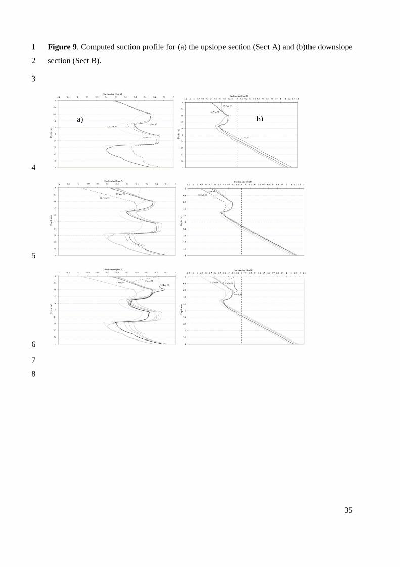
For each zone, the temporal distribution of suction profiles is drawn (Figure 9) plotting, in 1

particular, the most critical profile computed for each month. 2

From Figure 9a it is evident that water table is not present at the top of the slope, since the 3

values of the pressure head in the section are always lower than zero. This situation is fully 4

congruent with the morphological characteristics of the zone, where steep slopes do not allow 5

any form of accumulation. The situation is different for the Section B (Figure 9b), where the 6

lower layers reach saturated conditions, and the upper ones present higher values close to 7

saturation on 5th May. These results suggest that the saturation of the underlying layers was 8

not the only cause of the instability of the slopes, even if it contributes to this phenomenon. 9

In fact, the suction levels seem to have played an important role for the mudflows occurred in 10

May 1998. The values of rainfall heights during those days were not so extreme, but certainly 11

unusual for a late spring period. The suction values achieved on May 1998 in the lower layers 12

are not singular values: on the contrary, in previous periods the model provided quite similar 13

distributions. The main difference lies in the fact that on 5th May 1998, the vertical profiles of 14

water content present conditions close to saturation of the shallow layers. 15

This result is even more evident by analyzing the pressure profile along the slope and over the 16

whole period considered. Figure 10 shows the pore-water pressures performed at 3 m and 0.7 17

m below the ground level. The first case represents a typical situation of a relatively deep 18

layer, which reaches saturation in the first months of the rainy season and the second is 19

representative of the conditions in the upper layers. 20

In the lower layers (Fig. 10a), the pressure levels remain approximately the same with the 21

rainfall in late April and early May, while the upper layers (Fig.10b) get a sharp increase on 22

May 5 . The values reached in the month of May in the lower layers are not singular values, in 23

contrast, already at other times, the model refers distributions quite similar. 24

The substantial difference lies is that ever, as for May 5, in these distributions were added 25

conditions close to saturation of the surface layers. 26

In relation to the computed pore pressure, slope stability analysis was carried out to simulate 27

failure conditions and their correlation with increasing of soil water content. 28

Specifically, their effects on the stability were evaluated along several potential slip surfaces 29

combining the results with infinite slope analysis methods, in order to present a predictive 30

formulation of slope failures that occur as a result of rainfall events. In details, the analysis 31

18

was evaluated in both saturated and unsaturated conditions by using an extension of Mohr-1

Coulomb criterion; at different depths from the ground surface the average value of pore 2

pressure was calculated, and the correspondent value of FS was estimated using the method of 3

infinite slope. 4

In details, for several depth from the ground level (0.3m, 0.7m, 1.8m, 2.1 m, 2.9m, 3.1m, 5

3.8m) the average value of pore pressure was calculated, and then the correspondent value of 6

FS was estimated using the method of infinite slope. This method is the simplest limit 7

equilibrium method for slope stability analysis and gives reliable results for slides where the 8

longitudinal dimension prevails on the depth of the landslide, as for the landslide here 9

analyzed. 10

The plots in Figure 11 provide the time sequence of the simulated FS values; these results can 11

help in understanding the evolution of the slope stability conditions. 12

The values in the lower layers are always indicative of stability; lower values, but 13

nevertheless above 1, are due to the greater thicknesses of coverage and higher values of pore 14

pressure. In the more superficial layers the trends are more variable and reveal a depth of 15

0.7m, a decrease of FS value of 0.98 on May 5, 1998. 16

This result seems to be interesting, because suggest the hypothesis that the saturation of these 17

deep layers is not the only reason of the slopes instability in the investigated context but, 18

certainly, contributes to this phenomenon. The rainfall occurred on May 98, though not 19

exceptional, are unusual for late spring; they significantly increased the level of pore water 20

pressure in the upper layers, leading to a condition of instability. 21

22

5 Conclusions 23

The proposed SUSHI model is able to represent, with sufficient details, the phenomena 24

induced by rainfall, in soils characterized by complex stratigraphy and hydraulic properties, 25

and represents a complete model for water circulation analysis. 26

The application in the selected slope of Sarno area (Southern Italy) has enabled the 27

reconstruction of the full development of pore pressures in colluvial layers and to distinguish 28

the conditions occurred on May 1998 from the previous ones, thus providing important 29

information to identify the possible critical conditions of these slopes. In particular, by 30

analyzing the obtained results, the role of the suction appears to have been decisive for the 31

19

triggering of landslide movements, consistently with the most reliable theories that attribute to 1

the dynamics of water circulation in the surface soils a primer role either for the triggering 2

phase and the subsequent propagation phase. 3

Further applications to cases recorded on 5th May 1998 and periods without landslides could 4

certainly better delineate the critical conditions and provide useful information for a possible 5

early warning system. As well further analyses should be carried out in order to better 6

evaluate the influence of the bedrock, of the road cuts located in the upper zone of the 7

triggering areas, and other factors that could have influenced the evolution of events. 8

9

10

11

20

References 1

Arnone, E., Noto, L.V., Lepore, C., and Bras, R.L.: Physically‐based and distributed approach 2

to analyze rainfall‐triggered landslides at watershed scale, Geomorphology, n/a. doi: 3

10.1016/j.geomorph.2011.03.019, 2011 4

Baum, R.L., Savage, W.Z., and Godt, J.W.: TRIGRS - a FORTRAN program for transient 5

rainfall infiltration and grid-based regional slope stability analysis, US Geological Survey 6

Open-File Report, 02-0424, 2002 7

Baum, R.L., Godt, J.W., and Savane, W.Z.: Estimating the timing and location of shallow 8

rainfall-induced landslides using a model for transient, unsaturated infiltration, J. Geophys. 9

Res.,115:1-26, 2010. 10

Caine N.: The rainfall intensity-duration control of shallow landslides and debris flows, 11

Geogr. Ann. 62A(1-2):23-27, 1980. 12

Iverson, R.M.: Landslide triggering by rain infiltration, Water Resour Res, 36: 1897-1910, 13

2000. 14

Capparelli G. and Tiranti D. Application of the MoniFLaIR early warning system for rainfall-15

induced landslides in the Piedmont region (Italy). Landslides 7 n.4, 401-410; Springer-Verlag. 16

(2010) DOI: 10.1007/s10346-009-0189-9 17

Capparelli, G., and Versace, P.: FLaIR and SUSHI: Two mathematical models for Early 18

Warning Systems for rainfall induced landslides, Landslides, 8: 67‐79, 2011. 19

Cascini L, Cuomo S, Guida D:Typical source areas of May 1998 flow-like mass movements 20

in the Campania region, Southern Italy. Eng Geol 96:107–125, 2008. 21

Calcaterra D., Parise M., Palma B. e Pelella L.: Multiple debris flows in volcanoclastic 22

materials mantling carbonate slopes. Atti 2nd Int. Conf. “Debris-FIow Hazard Mitigation”, 23

Taipei, Taiwan, 16-18 Luglio 2000, pp. 99-107. 2000. Balkema, Rotterdam. 24

Celico, P., Guadagno, F. M., Vallario, A.: Proposta di un modello interpretativo per lo studio 25

delle frane nei terreni piroclastici, Geologia Applicata e Idrogeologia, 22, Bari, 1986 26

Dhakal, A.S. and Sidle, R.C. Pore water pressure assessment in a forest watershed: 27

Simulations and distributed field measurements related to forest practices. Water Resources 28

Research 40. (2004). doi: 10.1029/2003WR002017 29

21

D'Odorico, P., Fagherazzi, S. and Rigon, R. Potential for landsliding: Dependence on 1

hyetograph characteristics. Journal of Geophysical Research 110. (2005). doi: 2

10.1029/2004JF000127. 3

Ellen S.D., Fleming R.W. (1987): Mobilization of debris flow from soil slips, San Francisco 4

Bay region, California, Engineering Geology, 7 , 31-40. 5

Fredlund, D.G., and Rahardjo, H.: Soil Mechanics for Unsaturated Soils, John Wiley & Sons, 6

1993. 7

Fredlund, D.G., and Xing, A.: Equations for the soil-water characteristic curve, Can Geotech 8

J, 31:521-532, 1994. 9

Freeze. RA. 'Mathematical models of hillslope hydrology", in Kirkby, MJ (Ed.), Hillslope 10

Hydrology, John Wiley & Son 177-226., 1978. 11

Glade T. (2000): Modelling landslide-triggering rainfalls in different regions in New Zealand 12

- the soil water status model.- Zeitschrift für Geomorphologie 122, 63-84. 13

Greco R., Comegna, L., Damiano E., Olivares, L., Picarelli L,:Hydrological modelling of a 14

slope covered with shallow pyroclastic deposits from field monitoring data. Hydrol. Earth 15

Syst. Sci. Discuss., 10, 5799–5830, 2013 doi:10.5194/hessd-10-5799-2013 16

Guzzetti, F.: Book Review of “Measuring Vulnerability to Natural Hazards”, Nat. Hazards 17

Earth Syst. Sci. 8, 521, 2008. 18

Iverson, R.M.: Landslide triggering by rain infiltration, Water Resour Res, 36: 1897-1910, 19

2000. 20

Lu N. and Godt J. “Hillslope Hydrology and Stability” , Cambridge University Press, 2013 21

Martelloni G, Segoni S, Fanti R et al., 2011. Rainfall thresholds for the forecasting of 22

landslide occurrence at regional scale. Landslides, doi: 10.1007/s10346-011-0308-2. 23

Mazzoleni, S., Strumia, S., Di Pasquale, G., Migliozzi, A., Amato, M., Di Martino, P.: Il ruolo 24

della vegetazione nelle frane di Quindici. Tratto da: “L’instabilita` delle coltri piroclastiche 25

delle dorsali carbonatiche in Campania: primi risultati di uno studio interdisciplinare”. 20 26

Rapporto informativo dellUnita`Operativa 4/21N del CNR/GNDCI, 1998. 27

Montgomery, D.R. and Dietrich, W.E: A physically based model topographic control on 28

shallow landsliding, Water Resour Res, 30: 1153-1171, 1994. 29

22

Olivares, L. and Picarelli, L.: Shallow flowslides triggered by intense rainfalls on natural 1

slopes covered by loose unsaturated pyroclastic soils, Géotecnique, 53(2): 283-288, 2003. 2

Pack, R.T., Tarboton, D.G. and Goodwin, C.N.: SINMAP, a stability index approach to 3

terrain stability hazard mapping, SINMAP user’s manual, 68, Terratech Consulting Ltd, 1998. 4

Paniconi, C., Putti, M.,. A comparison of Picard and Newton iteration in the numerical 5

solution of multidimensional variably saturated flow problems. Water Resources Researches, 6

30, No 12, 3357-3374,1994 7

Rahardjo, H., Li, X.W., Toll, D.G., Leong, E.C., 2001, The effect of antecedent rainfall on 8

slope 9

stability. Geotechnical and Geological Engineering 19, 371–399 10

Revellino P, Hungr O, Guadagno FM, Evans SG: Velocity and runout simulation of 11

destructive debris flows and debris avalanches in pyroclastic deposits, Campania region, Italy. 12

Environ Geol 45:295–311,2004. 13

Rigon, R. Bertoldi, G. and Over, T.M. 2006: GEOtop: A Distributed Hydrological Model 14

with Coupled Water and Energy Budgets. J. Hydrometeor, 7, 371–388. 15

Rolandi G. The eruptive history of Somma-Vesuvius volcanism and archeology in 16

Mediterranean area. De Vito and Cortini (eds) 1997 17

Sorbino G., Sica C., Cascini L. Susceptibility analysis of shallow landslides source areas 18

using 19

physically based models. Natural hazards, 53(2), 313-332 (2010). 20

Srivastava R., Jim Yeh T.C.,. Analytical Solution for One-Dimensional, Transient Infiltration 21

Towards the Water Table in Homogeneous and Layered Soils. Water Resources Research, 22

27(5): 753-762, 1991 23

Tsai, T. L, Chen, H.E. and Yang, J.C.: Numerical modeling of rainstorm induced shallow 24

landslides in saturated and unsaturated soils, Environmental Geology 55:1269-1277, 2008. 25

Vanapalli, S.K., Fredlund, D.G., Pufahl, D.E., and Clifton, A.W.: Model for the prediction of 26

shear strength with respect to soil suction, Can. Geotech. J., 33, 379-392, 1996. 27

Van Genuchten, M.T., and Nielsen, D.R.: On describing and predicting the hydraulic 28

properties of unsaturated soils, Ann Geophys 3(5): 615-628, 1985. 29

23

Van Westen, C. J., Rengers, N., and Soeters, R.: Use of geomorphological information in 1

indirect landslide susceptibility assessment, Natural Hazards, 30, 399–419, 2003. 2

Vauclin, M., Khanji, D. e Vachaud, G.,. Experimental and numerical study of a transient, two-3

dimensional unsaturated-saturated water table recharge problem. Water Resources 4

Researches, 15, No 5, 1089-1101, 1979 5

Wu, W., and Sidle, R.C.: A distributed slope stability model for steep forested basin, Water 6

Resource Res 31: 2097-2110, 1995. 7

8

9

24

1

Table 1. Features of some recent flowslides in Campania Region (Versace et al., 2009) 2

3

4

5

6

7

8

9

10

11

12

13

14

15

16

17

18

19

20

21

22

23

24

25

Site Date Length (m) Volume (m3)

Ischia 2006 450 3*104

Cervinara 1999 2*103 4*104

Avella 1998 15*102 2*104

S. Felice a C. 1998 8*102 3*104

Sarno 1998 2-4*103 5*105

Bracigliano 1998 1-2*103 15*104

Siano 1998 14*102 4*104

Quindici 1998 1-4*103 5*105

Maiori 1954 103 5*104

Avellino 2005 4*102 2*104

Montoro Inf. 1997 2*103 3*104

25

Table 2. Comparison between monthly mean and daily maximum rainfall, computed for the 1

period 1964-1997 and the year 1998 2

3

  Jan.  Feb.  Mar.  Apr.  May  June  July  Aug.  Sept.  Oct.  Nov.  Dec. 

Monthly expected

value (mm)

1964/1997

87 85 73 73 38 26 18 27 60 104 129 111

1998 77 46 44 109 150 12 6 39 122 52 124 94

Daily maximum

(mm) 29 24 23 22 15 13 9 16 27 32 38 34

1998 42 21 13 37 74 6 5 20 47 17 25 37

4

5

6

26

Table 3. Average values of pyroclastic soil properties 1

2

3

4

Top

Soil

Pumice

(A)

Paleosoil

(B)

Pumice

(C)

Paleosoil

(D)

Regolite

(E) Soil properties

Dry unit weight [kN/m3] 10.99 6 7 6 9 10.75

Saturated unit weight [kN/m3] 17.2 13 13 13 15 15.3

Saturated soil water content s 0.55 0.82 0.61 0.68 0.61 0.60

Residual soil water content r 0.14 0.23 0.18 0.05 0.18 0.10

Saturated hydraulic conductivity Ks

[m/sec] 3.2E-05 1.0E-03 1.0E-06 1.0E-02 4.0E-06 7.6E-07

Effective coesion c’[kPa] 2 0 4.5 0 4.7 15

Friction angle ’ [°] 15 30 24 32 28 21

27

1

Figure 1. Nodal network implemented for development of FDM equation. 2

3

4

5

6

7

8

9

10

11

12

13

A

B

D

C

transient flux

(i,j) (i+1,j) (i-1,j)

(i,j-1)

(i,j+1)

X=ix

Z=jz

x

z

28

1

2

Figure 2. Overview of Pizzo d’Alvano massif and the area affected by the May 1998 mud 3

flows. Red square delimits the analyzed event by Sushi model 4

5

6

7

8

9

10

11

12

13

14

15

16

17

18

Pizzo d’Alvano

Sarno

Siano

Bracigliano

Quindici

Landslides

(May, 1998)

29

1

Figure 3. Topography map and sites where suction measurements were performed. 2

3

4

5

Pizzo d’Alvano

30

Figure 4. Suction trends recorded along sites at 0.20 m (a), 1.00 m (b), 1.60m (c) under the 1

ground surface and daily rainfall by Santa Maria la Foce rain-gauge. 2

3

4

5

6

7

a)

b)

c)

31

Figure 5. Comparison of daily and cumulative rainfall data recorded at Sarno- rain gauge in 1

1998. 2

3

4

32

Figure 6. Detail pictures of case study. 1

2

3

4

5

6

7

8

9

10

11

12

13

14

15

16

17

18

725 m a.s.l.

500 m a.s.l.

Outcropping bedrock scarps

33

Figure 7. Geometric and stratigraphic characterization of the investigated slope 1

2

3

4

5

6

7

8

9

Bedrock

Z(m a.s.l.)

34

Figure 8 Soil water characteristic curves 1

2

3

4

5

6

7

8

upper pumice layer

lower pumice layer

paleosoil

35

Figure 9. Computed suction profile for (a) the upslope section (Sect A) and (b)the downslope 1

section (Sect B). 2

3

4

5

6

7

8

a) b)

36

Figure 10 Pore-water pressures performed at (a) 3 m and (b) 0.7 m below the ground surface. 1

2

3

4

5

6

a)

b)

37

1

Figure 11 Slope safety factor depending on pore-water pressures performed and soil 2

mechanism properties at different depths from the ground surface. 3

4

5