Nonlinear velocity redistribution caused by energetic-particle-driven geodesicacoustic modes, mapped with the beam-plasma system

A. Biancalani1, N. Carlevaro2,3, A. Bottino1, G. Montani2,4, and Z. Qiu5

1 Max Planck Institute for Plasma Physics, 85748 Garching, Germany2 ENEA, Fusion and Nuclear Safety Department, C. R. Frascati, Via E. Fermi 45, 00044 Frascati (Roma), Italy

3 LTCalcoli Srl, Via Bergamo 60, 23807 Merate (LC), Italy4 Physics Department, “Sapienza” University of Rome, P.le Aldo Moro 5, 00185 Roma (Italy)

5 Institute for Fusion Theory and Simulation and Department of Physics, Zhejiang University, 310027 Hangzhou,People’s Republic of China

contact of main author: www2.ipp.mpg.de/~biancala

Abstract

The nonlinear dynamics of energetic particle (EP) driven geodesic acoustic modes (EGAM)in tokamaks is investigated, and compared with the beam-plasma system (BPS). The EGAMis studied with the global gyrokinetic (GK) particle-in-cell code ORB5, treating the thermalions and EP (in this case, fast ions) as GK and neglecting the kinetic effects of the electrons.The wave-particle nonlinearity only is considered in the EGAM nonlinear dynamics. TheBPS is studied with a 1D code where the thermal plasma is treated as a linear dielectric, andthe EP (in this case, fast electrons) with an n-body hamiltonian formulation. A one-to-onemapping between the EGAM and the BPS is described. The focus is on understanding andpredicting the EP redistribution in phase space. We identify here two distinct regimes for themapping: in the low-drive regime, the BPS mapping with the EGAM is found to be complete,and in the high-drive regime, the EGAM dynamics and the BPS dynamics are found to differ.The transition is described with the presence of a non-negligible frequency chirping, whichaffects the EGAM but not the BPS, above the identified drive threshold. The difference canbe resolved by adding an ad-hoc frequency modification to the BPS model. As a main result,the formula for the prediction of the nonlinear width of the velocity redistribution around theresonance velocity is provided. This article is written as the second of a series of articles (thefirst being Ref. [1]) on the saturation of EGAMs due to wave-particle nonlinearity.

1 Introduction

Zonal (i.e. axisymmetric) flows, associated to zonal radial electric fields, are often observed inturbulent tokamak plasmas, driven by the nonlinear interaction with drift-wave turbulence intokamaks. Both zero-frequency zonal flows (ZFZF) [2, 3, 4] and finite frequency geodesic acousticmodes (GAM) [5, 6, 7] can be excited. GAMs have an oscillatory character, as they are basicallya sound standing wave in the nonuniform tokamak magnetic field (the toroidal curvature beingthe main nonuniformity). GAMs are characterized by a dominant m=0 perturbed radial electricfield and dominant m=1 perturbed density (m being the poloidal mode number). Due to theiroscillatory character with frequencies of the order of the ion transit frequency, they are stronglyaffected by Landau damping (whereas ZFZF are mainly damped by collisional damping). As aconsequence of this energy flow from microscopic to mesoscopic scales, ZFZFs and GAMs play arole as major turbulence saturation mechanisms. Moreover, in the presence of energetic particles(EP), EP-driven GAMs (EGAM) can be driven unstable due to inverse Landau damping. EGAMshave been studied theoretically [8, 9, 10, 11, 12, 13, 14, 16, 17, 7] and experimentally (see forexample Ref. [18]). The role of EGAMs as possible mediators between EP and turbulence hasalso been emphasized [12, 16]. One of the main effects of EGAMs in tokamak plasmas is the

1

redistribution of the EP population (crf. Ref. [19] for the implications on the losses of counter-passing EP). In particular, in phase space, this occurs due to nonlinear inverse Landau damping.As a possible consequence, EGAMs might modify the efficiency of the heating mechanism ofneutral beam injectors or ion cyclotron heating.

A kinetic model is necessary for theoretically describing the EGAM. One reason is that theEGAM has a frequency of the order of magnitude of the sound frequency ωs =

√2cs/R0, with cs =

√

Te/mi being the sound speed (with Te the electron temperature and mi the thermal ion mass)and R0 being the major radius, and this is comparable to the transit frequency of thermal ions:therefore, resonances with the thermal ions substantially modify the EGAM frequency. Anotherreason is that the damping and excitation mechanisms, i.e. respectively the Landau damping andthe inverse Landau damping, are intrinsically wave-particle mechanisms. Moreover, resonanceswith electrons are found to be important for a proper determination of the damping/growthrates of modes of the family of the GAM, and therefore, when a comparison of the theoreticalpredictions with experiments is desired, kinetic effects of electrons should also be retained [20, 21].Due to the fact that numerical simulations in 3D real space and 3D velocity space are numericallytoo demanding for the present computational capabilities, and include much physics which isnot interacting with the EGAM due to separation of scales, it is desirable to reduce the modelcomplexity. Due to the fact that the EGAM frequency is much lower than the ion gyro-frequency,a reduction is possible from 6D to 5D in phase space, with the gyrokinetic (GK) model. Thisstrongly reduces the computational times. Nevertheless, a comparison with even more simplifiedreduced models is essential to identify the basic physics of the selected instability, and to pushtowards modeling techniques which can act in real-time, in parallel to a tokamak discharge. Suchare 1D reduced models.

In this article, we investigate the nonlinear dynamics of EGAMs due to wave-particle nonlin-earity. A strong analogy between the EGAM and the beam-plasma system (BPS) [22, 23] exists(see [10, ?]). Although the BPS is basically a mono-dimensional (1D) problem, and the corre-sponding unstable wave, i.e. the Langmuir wave, lives in a higher frequency domain, neverthelessboth instabilities are driven by a suprathermal species (fast ions for the EGAM, fast electronsfor the BPS) via inverse Landau damping. Moreover, although the EGAM is a 2D problem in anequilibrium toroidal magnetic field, its excitation mechanism, i.e. the inverse Landau damping,acts mainly in one direction, namely the direction parallel to the local equilibrium magnetic field.Therefore, once a proper mapping is made, both instabilities can be investigated in terms of aninverse Landau damping problem in a 1D system. As a consequence, not only the linear dynamics,but also the nonlinear wave-particle dynamics has strong analogies for the two instabilities. Inparticular, the bounce frequency of the EP which fall trapped into the perturbed electric field isproportional to the square root of the perturbed electric field [10, 24], and the saturated electricfield is proportional to the square of the linear growth rate [1, 24]. As a consequence, the questionarises whether also the EP redistribution in phase space can be described with similar models forboth instabilities.

The comparison of the nonlinear EP redistribution in velocity for the EGAM and the BPS isthe problem faced in this article. The EGAM is studied here with the global GK particle-in-cellcode ORB5, which was developed in tokamak geometry for electrostatic turbulence studies [25]and now includes the electro-magnetic multi-species extensions [26, 27]. ORB5 has been verifiedagainst analytical theory [28] and benchmarked against GYSELA [29] and GENE [17] for thelinear dynamics of EGAMs. Moreover, the scaling of the saturated electric field of EGAMs withthe linear growth rate, for saturation due to wave-particle nonlinearity, has been studied with

2

ORB5 [1]. The BPS is studied here with a 1D code treating the thermal plasma as a cold dielectricmedium and describing the dynamics of the fast electrons as an N-body problem solved with anHamiltonian formulation [30, 31, 32]. A mapping of the velocity space for the EGAM system andfor the bump-on-tail (BoT) paradigm for the BPS is also formulated, allowing to find a one-to-onecorrespondence between EP redistribution studied in the two problems.

Two regimes are identified here: the regime where the instabilities are weakly driven shows avery good match between the nonlinear EP redistribution observed in the two problems; on theother hand, above a certain threshold in the drive, a difference is found. The difference occursdue to the nonlinear modification of the mode frequency (i.e. the frequency chirping) which existsfor the EGAMs, but is not observed for the BPS for the cases of interest. This frequency chirpingis observed here to shift the resonance velocity of the EGAM, whereas the resonance velocity ofthe BPS remains constant in time. As a consequence, the EP redistribution for strongly drivenEGAM is observed to affect a region of the velocity space which slightly moves in time, creatinga qualitatively different picture. It is important to note that the scaling of the saturated electricfield with the linear growth rate was found to be quadratic in Ref. [1], and it does not changeat the threshold of the two regimes identified here. Therefore, we can state that the onset ofa non-negligible frequency chirping affects the EP redistribution in velocity space but not thescaling of the saturated levels. The EP redistribution of the EGAM is shown to be recoveredwith the BPS in the high-drive regime, by adding an ad-hoc frequency modification to the BPSmodel. As a main result, the formula for the prediction of the nonlinear width of the velocityredistribution around the resonance velocity is provided, and a good match with GK simulationsis found.

The article is organized as follows. In Sec. 2, the gyrokinetic model of ORB5 used here for thestudy of the EGAM is introduced. In Sec. 3, the equilibrium is defined and the linear dynamicsof EGAMs is described. The time evolution of the EGAM is shown in Sec. 4. Sec. 5 is devoted toa description of the analogy between the EGAM and the BPS, and the definition of the mapping.The mapping is applied to the prediction of the EP redistribution in velocity space, which is givenin Sec. 6, together with the discussion of the regimes of validity.

2 The gyrokinetic model

The EGAM problem is investigated here with the global nonlinear GK particle-in-cell code ORB5.ORB5 was written for studying electrostatic turbulence in tokamak plasmas [25], and extendedto treat multiple kinetic species (i.e. thermal ions, electrons, EP, impurities, etc) and electromag-netic perturbations [26, 27]. A collision operator is also implemented in ORB5, for the linearizedinclusion of inter-species and like-species collisions. In this article, electrostatic collisionless simu-lations are performed with ORB5. Only the wave-particle nonlinearity is considered, by filteringout all n 6= 0 modes and pushing only the EP species along the perturbed trajectories (whereasthe bulk ions and electrons follow the unperturbed trajectories).

The model equations of the electrostatic version of ORB5 are the marker trajectories, and thegyrokinetic Poisson law regulating the evolution in time of the scalar potential φ. These equationsare derived in a Lagrangian formulation [33]. The equations for the marker trajectories for the

3

thermal ions and fast ions (in the electrostatic version of the code) are [27]:

R =1

msp‖

B∗

B∗‖

+c

qsB∗‖

b×[

µ∇B + qs∇φ]

(1)

p‖ = −B∗

B∗‖

·[

µ∇B + qs∇φ]

(2)

µ = 0 (3)

The set of coordinates used for the phase space is (R, p‖, µ), i.e. respectively the gyrocenterposition, canonical parallel momentum p‖ = msv‖ and magnetic momentum µ = msv

2⊥/(2B)

(with ms and qs being the mass and charge of the species). v‖ and v⊥ are respectively the paralleland perpendicular component of the particle velocity. We label the gyroaverage operator withthe tilde symbol . B∗ = B+ (c/qs)∇× (b p‖), where B and b are the equilibrium magnetic fieldand magnetic unitary vector.

As we are not interested here in comparing the EGAM damping/growth rates with experi-mental observations, but only in investigating a specific piece of the nonlinear physics of EGAMs,we neglect kinetic effects of the electrons. This is done by calculating the electron gyrocenterdensity directly from the value of the scalar potential as [27]:

ne(R, t) = ne0 +ene0

Te0

(

φ− φ)

(4)

where φ is the flux-surface averaged potential, instead of treating the electrons with markersevolved with Eqs. 1, 2, 3.

We are interested here in the dynamics of zonal perturbations, and we filter out all non-zonalcomponents. We are not interested here in the wave-wave coupling, and therefore we push thebulk-ion and electron markers along unperturbed trajectories. This means that, in Eqs. 1, 2,3 for the bulk ions, the last terms, proportional to the EGAM electric field, are dropped. Onthe other hand, we push the EP markers along the trajectories which include perturbed termsassociated with the EGAM electric field. This means that the EP markers are evolved withEqs. 1, 2, 3 where the terms proportional to the EGAM electric field are retained. This retainsthe wave-particle nonlinearity of the EP.

Finally, the gyrokinetic Poisson equation is [27]:

−∑

s 6=e

∇ · n0smsc2

B2∇⊥φ =

∑

s 6=e

∫

dWsqs ˜δfs + qene(R, t) (5)

with n0s =∫

dWsf0s. The summation over the species is performed for the bulk ions and for theEP, whereas the electron contribution is given by qene(R, t). Here δfs = fs−f0s is the gyrocenterperturbed distribution function, with fs and f0s being the total and equilibrium (i.e. independentof time, assumed here to be a Maxwellian) gyrocenter distribution functions. The integrals areover the phase space volume. The phase-space volume element is dWs = (2π/m2

s)B∗‖dp‖dµ being

the velocity-space infinitesimal volume element. In this article, finite-larmor-radius effects areconsidered, for both thermal and fast ions.

3 Equilibrium and linear EGAM dynamics

We consider here the same tokamak configuration adopted in Ref. [1], where the scalings of theEGAM nonlinear saturation levels were studied. The tokamak magnetic equilibrium is defined by

4

0 5 10 15 20 25 300.9

1

1.1

1.2

1.3

1.4

1.5

1.6

1.7

1.8

nEP

/ni [%]

ωL [2

1/2

vti / R

]EGAM frequency

GAM (theory, q=2)

ORB5, q=2, ρ*=0.0078, kr ρ

i=0.035

0 5 10 15 20 25 30−0.02

0

0.02

0.04

0.06

0.08

0.1

nEP

/ni [%]

γ L [2

1/2

vti / R

]

EGAM growth rate

ORB5, q=2, ρ*=0.0078, kr ρ

i=0.035

Figure 1: Linear frequency (left) and growth rate (right) vs EP concentration.

a major and minor radii of R0 = 1 m and a = 0.3125 m, a magnetic field on axis of B0 = 1.9 T,a flat safety factor radial profile, with q = 2, and circular flux surfaces (with no Grad-Shafranovshift). Flat temperature and density profiles are considered at the equilibrium. The bulk plasmatemperature is defined by ρ∗ = ρs/a, with ρs = cs/Ωi, with cs =

√

Te/mi being the soundspeed. We choose ρ∗ = 1/128 = 0.0078 (τe = Te/Ti = 1 for all cases described in this article),corresponding to 2/ρ∗ = 256.In the case of a hydrogen plasma, we get a value of the ion cyclotron frequency of Ωi = 1.82 · 108rad/s and a temperature of Ti = 2060 eV. The sound frequency is defined as ωs = 21/2vti/R (withvti =

√

Ti/mi, which for τe = 1 reads vti = cs). We obtain cs = 4.44 · 105 m/s. This correspondsto the following value of the sound frequency: ωs = 6.28 · 105 rad/s.

The energetic particle distribution function is a double bump-on-tail, with two bumps at v‖ =±vbump, like in Ref. [29, 1], labeled here as FEP . In this article, vbump = 4 vti is chosen. In order toinitialize an EP distribution function which is function of the constants of motion only, we neglectthe radial dependence of the magnetic field in v‖(µ,E,R) =

√

2(E − µB)/m/vti ≃ v‖(µ,E) inthe Vlasov equation (details are given in Ref. [28]). Neumann and Dirichlet boundary conditionsare imposed to the scalar potential, respectively at the inner and outer boundaries, s = 0 ands = 1.

The scan of linear simulations with different EP concentration, performed in Ref. [1], isreported here for completeness. This defines the linear dynamics of the system. The dependence ofthe linear frequency and growth rate on the EP concentration is shown in Fig. 1. For comparison,the GAM frequency for these parameters is ωGAM = 1.8ωs. The list of the parameters describedabove defines a regime where the EGAM comes continuously from a GAM, when increasing theEP concentration from zero. On the other hand, the EGAM would come from a Landau pole,for sufficiently larger values of q (see Ref. [28]).

4 Nonlinear EGAM evolution

In this Section, we describe the evolution in time of the nonlinear simulations of EGAMs per-formed with ORB5. Here, like in the rest of this article, the wave-particle nonlinearity only is

5

0 1 2 3 4

x 104

103

104

|∇ φ

(t)|

[V

/m]

t [Ωi

−1]

Radial electric field, nEP

/ni=0.10

0.26562

0.34375

0.42188

0.5

0.57812

0.65625

0.73438

2.5 3 3.5 4 4.5

1.5

2

2.5

3

3.5

x 10−3

v||/vth,i

f ve

l 2

D (

µ=0

)

Distr. func. (aver. in space), for nEP

/ni= 0.10

2000

10000

16000

18000

20000

22000

24000

26000

Figure 2: Radial electric field in time, at different radial positions (left), and EP distributionfunction at different times, vs parallel velocity (right) for an EGAM simulation with ORB5 withnEP/ni = 0.10.

considered. As an example, we consider a case with nEP/ni = 0.10. A zonal (i.e. axisym-metric) radial electric field is initialized at t=0, with an amplitude of the order of 103 V/m,and let evolve in time in a nonlinear simulation with ORB5. A typical simulation has a spatialresolution set by a grid of (ns,nchi,nphi)=(256, 64, 16) number of points respectively in the ra-dial, poloidal and toroidal direction, a time step of dt = 20Ω−1

i , and a number of markers of(ntoti, ntotEP ) = (107, 107) respectively for the thermal and fast ions. An initial linear phaseis observed, where the radial electric field grows exponentially in time. In this phase the linearfrequency and growth rate are measured and checked to match with the ones of the linear simu-lation: ωL = 1.24ωs, γL = 0.06ωs. Then, a nonlinear phase is entered, the growth rate graduallydecreases to zero, and the radial electric field saturates at t ≃ 2.5 · 104 Ω−1

i (see Fig. 2-a), whenthe electric field reaches a value of δEr ≃ 3.5 · 104 V/m. This value of the saturated electric fieldcan be compared with the prediction of Ref. [1]:

δEr,th =2RBβ2

0

ωGAMγ2L = 3.5 · 104V

m(6)

where the constant β0 = 2.66 is estimated in Ref. [1] for this regime. For the present equilibriumplasma profiles, the regime is defined by the value of q = 2, for which we have an EGAM whichcomes from a GAM (see also Sec. 3). We emphasize here that the quadratic scaling of the electricfield with the linear growth rate shown in Eq. 6 has been found to be valid for the whole consideredrange of EP concentrations (the same range used in Fig. 1). After the saturation, the EGAMenters a deep nonlinear phase (t > 2.5 · 104 Ω−1

i ), when the electric field starts decreasing inamplitude. In this article we are interested in the first nonlinear phase only, up to the saturation,and we leave the study of the deep nonlinear phase to another dedicated article. In particular,we focus here on the nonlinear modification of the EP distribution function at the time of thesaturation, and on the corresponding nonlinear modification of the EGAM frequency.

The EP distribution function redistributes in v‖ during the first nonlinear phase, causing a

6

0 1 2 3 4

x 104

103

104

|∇ φ

(t)|

[V

/m]

t [Ωi

−1]

Radial electric field, nEP

/ni=0.176

0.26562

0.34375

0.42188

0.5

0.57812

0.65625

0.73438

2.5 3 3.5 4 4.5

2.5

3

3.5

4

4.5

5

5.5

x 10−3

v||/vth,i

f ve

l 2

D (

µ=0

)

Distr. func. (aver. in space), for nEP

/ni= 0.176

2000

4000

6000

8000

10000

12000

14000

16000

18000

20000

Figure 3: Radial electric field in time, at different radial positions (left), and EP distributionfunction at different times, vs parallel velocity (right) for an EGAM simulation with ORB5 withnEP/ni = 0.176.

relaxation of the drive due to the inverse Landau damping. The EP distribution function of thissimulation is shown in Fig. 2-b). The redistribution of the EPs is observed to occur in a rangeof velocities between 2.5 vti and 4.5 vti. The EP distribution function does not change duringthe linear phase, and when entering the nonlinear phase, the redistribution occurs with higher-velocity EP moving towards lower values of v‖, as time increases. Therefore, negative values ofthe perturbed distribution function are measured at high velocities, and positive at low velocities.The resonance velocity can be calculated as v‖res = qRωEGAM = 3.5 vti, and can be measuredin Fig. 2-b as the velocity where the perturbed distribution function changes sign. We note thatthis velocity measured in Fig. 2-b, for this value of nEP/ni = 0.10, does not sensibly change inthe time range of interest.

Before moving further, we want to consider another case for comparison, with a strongerdrive, namely with nEP/ni = 0.176. The evolution in time of the radial electric field is shown inFig. 3-a. The linear frequency and growth rate is measured and checked to match with the onesof the linear simulation: ωL = 1.14ωs, γL = 0.094ωs. The saturated level of the radial electricfield is measured at δEr ≃ 0.8 · 105 V/m (in agreement with the prediction of Ref. [1]).

The EP distribution function of the case with nEP/ni = 0.176 is shown in Fig. 3-b, fordifferent times up to the saturation. Firstly, we note that the range of velocities affected bythe nonlinear modification is broader than that for the weaker drive. In fact, the redistributionof the EPs is observed to occur in a range of velocities between 2 vti and 5 vti. Secondly, wenote that the resonance frequency, which is calculated in this case from the linear frequency asv‖res = qRωEGAM = 3.2 vti, does not perfectly describe the velocity of the change of sign of theperturbed distribution function at all times. In fact, the resonance velocity is observed to growin time, from 3.2 vti to 3.5 vti.

The evolution of the resonance velocity in time is in relation with the EGAM nonlinearfrequency modification, i.e. the EGAM chirping. The perturbed EP distribution function can beplotted explicitly (see Fig. 4-a). The positive peak (clump) and the negative peak (hole) can beseen to form and evolve in time, becoming bigger and centered at higher and higher distancesfrom the linear resonance velocity. The location in velocity space of the peaks can be measured

7

1 2 3 4 5−1

−0.5

0

0.5

1

x 10−3

v||/vth,i

df vel 2D

(µ=

0)

Pert. distr. function (aver. in space), for nEP

/ni= 0.176

2000

4000

6000

8000

10000

12000

14000

16000

18000

20000

1 1.5 2

x 104

0.9

1

1.1

1.2

1.3

1.4

1.5

1.6

t [Ωi

−1]

ω [2

1/2

vti/R

]

Frequencies of v of the maximum and minumum of δ f

ω

res,vpar1

ωres,vpar2

ωlin

ωNL

Figure 4: Perturbed distr. funct. (left), for a case with nEP/ni = 0.176. The times are expressedhere in units of Ω−1

i . On the right, frequencies corresponding to the positive (red) and negative(blue) peaks of the EP perturbed distribution function. The measured EGAM freq. is also shownin green.

and translated into resonance frequencies as ω1,2 = v‖1,2/qR (see Fig. 4-b). When compared withthe measured EGAM frequency, we note that the nonlinear EGAM frequency modification atthe time of the saturation is described with a good approximation by the resonance frequency ofthe negative peak (hole). This relation offers the possibility to predict the nonlinear frequencyby approximating it with the frequency obtained by the velocity of the negative peak of the EPperturbed distribution function (see also Ref. [11]).

In the next section, Sec. 5, we introduce the beam-plasma system (BPS) and the map linkingthe BPS with the EGAM. This map shows how we can predict the EGAM EP redistribution invelocity space.

5 Dynamics of the energetic particles: analogy with the beam-

plasma system

In the EGAM system, the equilibrium magnetic field is not uniform but has a toroidal shape.In general, particles moving in a toroidal magnetic field can perform passing orbits, i.e. followthe magnetic field on both low-field side and high-field side, or perform banana orbits in thespace restricted to the low-field side of the tokamak. By construction, in the EGAM problemconsidered here, the energetic ions are initialized with a bump-on-tail distribution function (beamdistribution), with a relatively high parallel mean velocity along the equilibrium magnetic field,plus a smaller isotropic thermal distribution around the mean velocity. Due to the relativelyhigh parallel velocity, the time derivative of their toroidal angle never vanishes (and thereforebanana orbits of the EP in the low-field side are not considered in the present treatment). Duringtheir motion which is, to the leading order, directed along the equilibrium magnetic field, theyperform small drifts towards higher values of the minor radius, and then towards lower values ofthe minor radius, known as the curvature and grad-B drifts. These drifts have zero time average:this defines orbits with an average radial position plus a radial orbit width.

8

The radial electric field of the EGAM can exchange energy with the energetic particles, dueto their radial component of the trajectories, and in particular of the curvature drift [10]: vdc =(v2‖/ΩEP )B×∇B/B2. Due to the structure of the perturbed distribution function, the effective

parallel wavenumber of the EGAM is k‖ = 1/qR, the phase-angle is Θ = θ − ωEGAM t and its

normalized time derivative is Θ/ωEGAM = (v‖ − v‖r)/qR ωEGAM . In terms of the phase angle,the energetic particles experience a periodic electric field, and their harmonic motion can beexpressed as [10]:

Θ

ω2EGAM

= − ω2b

ω2EGAM

sinΘ , (7)

where ωb is the bounce frequency of the energetic particles in the potential created by the wave.Using these considerations, the analogy with respect to the 1D beam-plasma system (BPS) turnsout to be evident. In fact, the BPS is described as given by a Langmuir wave, excited by abeam of energetic electrons along a given direction x. The Langmuir wave has a perturbedelectric field directed along x, oscillating at the plasma frequency ωp =

√

nee2/meǫ0. In general,the Langmuir wave can be decomposed in Fourier in terms of the wavenumbers kℓ = ℓ(2π/L),where L is the periodicity length of the 1D space domain of the BPS, and ℓ is a positive integer(whereas the EGAM has only one possible wavenumber set by the equilibrium, as mentionedabove). Considering a single monochromatic wave with a chosen value of ℓ, we can focus on that,and we denote the wavenumber as k. The phase-angle Θ experienced by the electrons in the fieldof the Langmuir wave is thus Θ = kx − ωpt and the normalized variation in time of the phaseangle is Θ/ωp = k(v−vr)/ωp = kv/ωp−1, where the resonant velocity is defined as vr = ωp/k. Asa choice of nomenclature, we refer here to the velocities of the EGAM as v‖, and to the velocitiesof the BPS as v. Similarly, we refer to the wavenumbers of the EGAM as k‖ = 1/qR, and to thewavenumbers of the BPS as k.

In the following, we describe the detailed mapping procedure which links the EGAM frame-work with the BPS. As already mentioned, the dynamics of the EGAM model can be reducedin the parallel velocity direction and we start from the generic resonance condition written usingtwo suitable normalization constants ν1,2, i.e.,

v‖ − v‖0

ν1=

v − vrν2

, (8)

where we recall that the transit resonance velocity reads v‖res = qRωEGAM(nEP ). Using theintroduced above standard normalization ν1 = vti and, for the calculation of this Section, v‖ =v‖/vti, in the following, we denote with v‖min 6 v‖ 6 v‖max the domain of the positive bump ofenergetic particles. Imposing the boundary v‖min = 0 7→ vmin = 0, in order to map one singlebump of energetic particles with v‖ > 0, we get ν2 = vr/v‖r and the map finally writes

v =vrv‖r

v‖ . (9)

Let us now introduce the following normalization: v = ωp(2π/L)−1 u. In order to fix the dimen-

sionless resonant wavenumber ℓr, we use the condition k1vmax = ωp, with vmax = vrv‖max/v‖r,which characterize the spectral features (wavenumbers and periodicity length). This yieldsℓr = ℓ1v‖max/v‖r, and ℓr is determined arbitrarily fixing ℓ1 since v‖max and v‖r are given quantitiesfrom the EGAM system. We stress how the resonance condition can be rewritten as ℓrur = 1.

9

The map between the velocities of the two systems is now closed. The bump (positive part) ofthe EP is described by the shifted Maxwellian distribution function FEP (v‖) in velocity space [1].For modeling the EP distribution function of the EGAM in the BPS, let us now discretize thepositive bump of FEP (v‖) in n delta-like beams, equispaced in velocity space and located in v‖j(with j = 1, ..., n), and assign the numbers of particles Nj for each beam distributed according toFEP . The initial conditions on the distribution for BPS simulations are now given by Nj particleslocated at

uj = v‖j/(ℓr v‖r) . (10)

For the sake of completeness, we mention that, for the simulation of the BPS, we have set n = 600,ℓ1 = 400 and we have usedN = 106 total particles. The complete derivation of the BPS dynamicalequation used here, is described in [30, 31] (and refs. therein), and it can be specified for onesingle resonance as:

x′i = ui , u′i = i ℓr φr eiℓr xi + c.c. , φ′

r = −iφr +iη

2ℓ2rN

N∑

i=1

e−iℓr xi , (11)

where the particle position along the x direction is labeled by xi, with i = 1, ... N (N being thetotal particle number) normalized as xi = xi(2π/L). The Langmuir electrostatic scalar potentialφ(x, t) is expressed in terms of the Fourier component φr(k, t) and we have used: η = nB/np

(for the plasma density np assumed much greater than the beam one nB), τ = tωp (the primeindicates derivative with respect to this variable), φr = (2π/L)2eφr/mω2

p, φr = φre−iτ . Eqs.(11)

are solved using a Runge-Kutta (fourth order) algorithm. For the considered time scales and foran integration step h = 0.1, both the total energy and momentum (for the explicit expressions,see [30]) are conserved with relative fluctuations of about 1.4× 10−5.

The BPS is closed once the density of the beam (drive) is fixed. In order to quantitativelycompare the non-linear features of two systems, we now fix the bounce (trapping) frequency ωB

normalized to the mode frequency equal for the two schemes. For the BPS, the bounce frequencyresults proportional to the linear growth rate of the mode γL,BPS. The same occurs for the EGAMsystem, but with a proportionality factor depending on the EP density [1]. In particular, we get:

ωB,BPS

ωp= α

γL,BPS

ωp,

ωB,EGAM

ωL,EGAM= β(nEP )

γL,EGAM

ωL,EGAM. (12)

where α ≃ 3.3 (see well-known literature results [34, 35] and also [32]) while for the EGAM we haveβ = β0

√

ωL,EGAM/ωGAM , with β0 = 2.66 in this regime (see Sec. 3), and ωL,EGAM depending onthe EP density [1]. For the four selected EGAM simulations, we get β(0.07, 0.10, 0.176, 0.30) ≃[2.21, 2.17, 2.07, 1.98]. Using standard normalization for frequencies, i.e., γL,BPS = γL,BPS/ωp

and γL,EGAM = γL,EGAM/ωGAM , ωL,EGAM = ωL,EGAM/ωGAM and equaling the bounce frequen-cies, we finally get

γL,BPS =β

α

γL,EGAM

ωL,EGAM. (13)

This condition preserves the linear and nonlinear features of the two systems and it is used inthe evaluation for the drive of BPS simulations from the linear dispersion relation which formallyreads as

ǫ = 1−ω2p

ω2=

ηω2p

k2

∫

+∞

−∞dv

k ∂vFB(v)

kv − ω. (14)

10

0 1 2 3 4 5 6 7 80

0.5

1

1.5

2

2.5

x 10−3

v||/vth,i

f ve

l 2

D (

µ=0

)

Distr. func. for nEP

/ni= 0.07 and res. vel. at t=0 and at t=satur +− δ v

2000 4000 6000 80001000012000140001600018000200002200024000260002800030000

0 1 2 3 4 5 6 7 80

0.5

1

1.5

2

2.5

3

3.5x 10

−3

v||/vth,i

f ve

l 2

D (

µ=0

)

Distr. func., for nEP

/ni= 0.10 and res. vel at t=0 and at t=satur +− δ v

2000 4000 6000 8000100001200014000160001800020000220002400026000

Figure 5: Energetic particle distribution function averaged in space, and measured at µ ≃ 0, vsparallel velocity, for nEP/ni = 0.07 (left) and nEP/ni = 0.10 (right). The vertical dashed andcontinuous lines are the resonance velocity (center), with the borders of the nonlinear velocitypredicted by v‖res ±∆v‖NL.

where FB(v) is the initial beam distribution function. Here, the dielectric function ǫ can beexpanded near ω ≃ ωp to deal with Langmuir modes as in Eqs.(11), i.e., ǫ ≃ 2(ω − 1) (whereω = ω/ωp). Let us now use the expansion ω = ω0 + iγL,BPS, where ω0 is the real part of thenormalized Langmuir frequency ω. Using the linear character of the mapping which yields thenormalization FB(v) = κFEP (v‖) (with κ = const.), Eq.(14) can be written in terms of theEGAM system variables as

2(ω0 + iγL,BPS − 1)−ηv‖r

M

∫

+∞

−∞dv‖

∂v‖FEP

v‖/v‖r − ω0 − iγL,BPS

= 0 , (15)

where M =∫

+∞−∞ dv‖FEP . This equation is numerically integrated assuming Eq.(13), which

guarantees the requested features described above, and provides the drive parameter η closingthe map procedure.

6 Nonlinear EP redistribution of the EGAM, and comparison

with the beam-plasma model

In this section, we compare the results of the EP redistribution due to the EGAM, with theredistribution due to the beam-plasma system. In particular, we aim at predicting, from BPSinformations, the nonlinear parallel velocity spread in the positive bump of the distribution func-tion.

In the BPS, the single mode dynamics proceeds in an initial exponential mode growth followedby non-linear saturation. Here the particles get trapped and begin to bounce back and forth inthe potential well generating clumps. A measure of the clumps width ∆ucNL for a generic initialhalf-Gaussian velocity distribution, which can be directly extrapolated to the analysis of the

11

0 1 2 3 4 5 6 7 80

1

2

3

4

5

x 10−3

v||/vth,i

f ve

l 2

D (

µ=0

)

Distr. func., for nEP

/ni= 0.176 and res. vel at t=0 and at t=satur +− δ v

2000

4000

6000

8000

10000

12000

14000

16000

18000

20000

0 1 2 3 4 5 6 7 80

1

2

3

4

5

6

7

8

9x 10

−3

v||/vth,i

f ve

l 2

D (

µ=0

)

Distr. func., for nEP

/ni= 0.30 and res. vel at t=0 and at t=satur +− δ v

2000

4000

6000

8000

10000

12000

14000

16000

18000

Figure 6: Same as FIG.5 but for nEP/ni = 0.176 (left) and nEP/ni = 0.30 (right).

present work, has been evaluated in [32] for several cases outlining the following scaling rule asfunction of the linear drive:

∆ucNL/ur = (6.64 ± 0.12) γL. (16)

In order to include the dynamic role also of passing but nearly resonant particles [36], i.e. theregion involved in the effective wave particle power exchange, in the following analysis we con-sider as the proper nonlinear particle velocity spread the scaled quantity ∆uNL ≃ χ∆ucNL withχ ≃ 1.28. This estimate is derived [32] characterizing the active overlap of different non-linearfluctuations [37, 38] and corresponds to the finite distortion of the distribution function, includingeffects at the edges of the plateau (defined as the flattened region of the distribution function,mainly coinciding with the clump size). We finally obtain the desired formula for the predictionof the nonlinear velocity spread due to the EGAM:

∆v‖NL

v‖L,res= 8.5 γBPS

L (17)

and by substituting the value of γBPSL we obtain:

∆v‖NL

v‖L,res= 2.57

β0√ωGAM

γEGAML√ωL,EGAM

(18)

Eq. 18 has been derived for the EGAM system, using the scaling derived in Eq.(13) and thenormalized mapping of Eq. (10). For the regime of interest in this article, we have β0 = 2.66 [1],and ωGAM = 1.8ωs, therefore we obtain:

∆v‖NL

v‖L,res=

5.1√ωs

γEGAML√ωL,EGAM

(19)

Let us now analyze the predictivity of Eq. 18, simplified as in Eq. 19 for the regime ofinterest. Four different simulations are considered, with different values of energetic particle con-centration: nEP/ni ∈ [0.07, 0.10, 0.176, 0.30]. The corresponding linear frequencies and growth

12

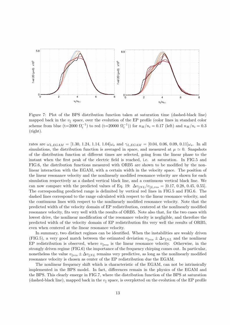
Figure 7: Plot of the BPS distribution function taken at saturation time (dashed-black line)mapped back in the v‖ space, over the evolution of the EP profile (color lines in standard color

scheme from blue (t=2000 Ω−1

i ) to red (t=20000 Ω−1

i )) for nH/ni = 0.17 (left) and nH/ni = 0.3(right).

rates are ωL,EGAM = [1.30, 1.24, 1.14, 1.04]ωs and γL,EGAM = [0.04, 0.06, 0.09, 0.11]ωs. In allsimulations, the distribution function is averaged in space, and measured at µ ≃ 0. Snapshotsof the distribution function at different times are selected, going from the linear phase to theinstant when the first peak of the electric field is reached, i.e. at saturation. In FIG.5 andFIG.6, the distribution functions measured with ORB5 are shown to be modified by the non-linear interaction with the EGAM, with a certain width in the velocity space. The position ofthe linear resonance velocity and the nonlinearly modified resonance velocity are shown for eachsimulation respectively as a dashed vertical black line, and a continuous vertical black line. Wecan now compare with the predicted values of Eq. 19: ∆v‖NL/v‖L,res = [0.17, 0.28, 0.45, 0.55].The corresponding predicted range is delimited by vertical red lines in FIG.5 and FIG.6. Thedashed lines correspond to the range calculated with respect to the linear resonance velocity, andthe continuous lines with respect to the nonlinearly modified resonance velocity. Note that thepredicted width of the velocity domain of EP redistribution, centered at the nonlinearly modifiedresonance velocity, fits very well with the results of ORB5. Note also that, for the two cases withlowest drive, the nonlinear modification of the resonance velocity is negligible, and therefore thepredicted width of the velocity domain of EP redistribution fits very well the results of ORB5,even when centered at the linear resonance velocity.

In summary, two distinct regimes can be identified. When the instabilities are weakly driven(FIG.5), a very good match between the estimated deviation v‖res ± ∆v‖NL and the nonlinearEP redistribution is observed, where v‖res is the linear resonance velocity. Otherwise, in thestrongly driven regime (FIG.6) the importance of the frequency chirping comes out. In particular,nonetheless the value v‖res ±∆v‖NL remains very predictive, as long as the nonlinearly modifiedresonance velocity is chosen as center of the EP redistribution due the EGAM.

The nonlinear frequency shift which is characteristic of the EGAM, can not be intrinsicallyimplemented in the BPS model. In fact, differences remain in the physics of the EGAM andthe BPS. This clearly emerge in FIG.7, where the distribution function of the BPS at saturation(dashed-black line), mapped back in the v‖ space, is overplotted on the evolution of the EP profile

13

for nEP/ni = 0.176 and nEP/ni = 0.3. In particular, it is evident how the discrepancy due thefixed character (at ∼ ωp) of the Langmuir resonance gives rise to a very different morphology ofthe distribution function, although well predicting the effective nonlinear velocity spread. Alsothe inclusion of additional modes with artificial ad hoc damping rates results in a drastically non-comparable non-linear dynamics, underlining the intrinsic differences of the physical systems.

7 Conclusions and discussion

Geodesic acoustic modes (GAMs), i.e. finite frequency zonal (i.e. axisymmetric) flows withmainly radial electric field polarization, are known to be important in tokamaks due to theirinteraction with turbulence. GAMs can also be excited by energetic particles (EPs), taking thename of EGAMs. In the view of understanding and predicting the EP redistribution in tokamaks,the linear and nonlinear dynamics of EGAMs should be properly theoretically understood.

In this article, we have investigated the nonlinear dynamics of EGAMs with particular inter-est in the EP redistribution in velocity space. As a tool of investigation of the nonlinear inverseLandau damping, which is responsible of the EGAM saturation and EP redistribution, a com-parison of the EGAM dynamics with the beam-plasma system (BPS) is done. Although the BPSdescribes the interaction of EP with a different mode, i.e. the Langmuir wave in a 1D geometry,nevertheless, analogies with the EGAM had been suggested in previous articles. These analogiesare investigated here and used to build a mapping of the two systems. The mapping is used tounderstand and predict the EP redistribution of the EGAM.

The EGAM is investigated here with collisionless electrostatic simulations with the gyroki-netic (GK) particle-in-cell code ORB5. Only the wave-particle nonlinearity is retained in thesimulations presented here, meaning that the markers for thermal ions follow unperturbed trajec-tories in phase space. The GK model allows to study the EGAM dynamics retaining the crucialphysics of the resonances with thermal and fast ions. The BPS is investigated with the a 1Dcode treating the thermal plasma as a cold dielectric medium and describing the dynamics ofthe fast particles (fast electrons in the case of the BPS) as an N-body problem solved with anHamiltonian formulation.

The GK simulations of the EGAM show that, after a first linear growth, the EGAM enters afirst nonlinear phase where the EP distribution function suffers a modification due to the EGAMfield. A saturation of the EGAM field occurs, and then a deep nonlinear phase is entered, wherenonlinear oscillations of the fields are observed. In this article, we are interested in the firstnonlinear phase only, up to the first saturation. The EP population is observed to redistribute,with EP going from higher to lower values of the parallel component of the velocity, as theEGAM grows in amplitude. The resonant velocity is also measured with ORB5 in the differentcases considered.

The mapping of the EGAM and the BPS is then described, and the comparison of the EPredistribution in velocity space is shown. In particular, the main result is the prediction of thewidth of the velocity space ∆uNL which is affected by the EGAM, around the resonance. Theimplication of this result is evident, as reduced models are needed for predicting the nonlineardynamics of instabilities in tokamaks, instead of using numerically expansive GK simulations.In fact, BPS simulations are numerically much cheaper, and therefore the mapping describedhere offers a tool for predicting the EP redistribution in regimes where EGAMs experience wave-particle nonlinear saturation.

14

We have also found a transition among two regimes: for weakly driven EGAMs, the resonantvelocity does not evolve in time during the first nonlinear phase, exactly like in the BPS problem;on the other hand, above a certain threshold in drive, the resonant velocity slightly increases intime, and therefore a difference of the EGAM and BPS is found. The increase of the resonantvelocity in the high-drive regime is consistent with the nonlinear frequency modification (i.e. thefrequency chirping) which is present for the EGAM, and is absent for the BPS considered here.The difference can be cured by calculating the nonlinear width ∆uNL around the new value ofthe resonant velocity. This proves that the one-to-one correspondence of the EP redistributionaround the resonance is completely described by the nonlinear inverse Landau damping which isincluded in the model of the BPS. Therefore, we can state that the EP are redistributed aroundthe resonance by the EGAM for a purely 1D problem which is the same as the BPS, namely thenonlinear inverse Landau damping. Having tried to include many modes in the BPS, we haveobserved that this can modify the EP redistribution, but leads to a overestimation of the EPredistribution due to a lack of damping in the different modes.

In the view of the continuation of this work, several next steps can be taken in the directionof getting closer to more and more realistic scenarios. For example, the inclusion of wave-wavecoupling of the EGAM with itself is under investigation. Kinetic electron effects should alsobe considered, as the electron resonances might affect the Landau damping. The inclusion ofturbulence is also in progress, as a mean of modifying the EGAM saturation level and EP redis-tribution.

Acknowledgements

Useful discussions with F. Zonca, P. Lauber, D. Zarzoso, I. Novikau, A. Di Siena, O. Gurcan andP. Morel are acknowledged. Useful discussions with L. Villard, and the whole ORB5 team, are alsoacknowledged. Part of this work has been carried out within the framework of the EUROfusionConsortium and has received funding from the Euratom research and training programme 2014-2018 under grant agreement No 633053, within the framework of the Nonlinear energetic particle

dynamics (NLED) European Enabling Research Project, WP 15-ER-01/ENEA-03 and Nonlinear

interaction of Alfvenic and Turbulent fluctuations in burning plasmas (NAT) European EnablingResearch Project, CfP-AWP17-ENR-MPG-01. The views and opinions expressed herein do notnecessarily reflect those of the European Commission. Simulations were performed on the Marconisupercomputer within the framework of the OrbZONE and ORBFAST projects. Part of this workwas done while one of the authors (A. Biancalani) was visiting ENEA-Frascati, whose team isacknowledged for the hospitality. This article, together with the companion article on EGAMsaturation and comparison with the beam-plasma-system (i.e. Ref. [1]), are dedicated to Prof.Francesco Pegoraro.

References

[1] A. Biancalani, I. Chavdarovski1, Z. Qiu, A. Bottino, D. Del Sarto, A. Ghizzo, O. Gurcan,P. Morel and I. Novikau J. Plasma Phys. 83 725830602 (2017)

[2] A. Hasegawa, C. G. Maclennan, and Y. Kodama, Phys. Fluids 22, 2122 (1979)

[3] M.N. Rosenbluth and F.L. Hinton, Phys. Rev. Lett. 80,4 724 (1998)

15

[4] P.H. Diamond, S.-I. Itoh, K. Itoh, and T. S. Hahm, Plasma Phys. Controlled Fusion 47, R35(2005)

[5] N. Winsor, J. L. Johnson, and J. M. Dawson, Phys. Fluids 11, 2448, (1968)

[6] F. Zonca and L. Chen, Europhys. Lett. 83, 35001 (2008)

[7] Z. Qiu, L. Chen and F. Zonca, Plasma Sci. and Technol. 20, 094004 (2018)

[8] G. Y. Fu Phys. Rev. Lett. 101 (18), 185002 (2008)

[9] Z. Qiu, F. Zonca, and L. Chen Plasma Phys. Control. Fusion 52 (9), 095003 (2010)

[10] Z. Qiu, F. Zonca, L. Chen Plasma Science and Tech. 13, 257 (2011)

[11] H. Wang, Y. Todo, and C. C. Kim, Phys. Rev. Lett. 110 (15), 155006 (2013)

[12] D. Zarzoso, et al. Phys. Rev. Lett. 110 (12), 125002 (2013)

[13] K. Miki, and Y. Idomura Plasma Fusion Res. 10, 3403068 (2015)

[14] D. Zarzoso, P. Migliano, V. Grandgirard, G. Latu and C. Passeron, Nucl. Fusion 57 072011(2017)

[15] M. Sasaki, N. Kasuya, K. Itoh, K. Hallatschek, M. Lesur, Y. Kosuga, and S.-I. Itoh Phys.

Plasmas 23 (10), 102501 (2017)

[16] M. Sasaki, et al. Scientific Reports 7, 16767 (2017)

[17] A. Di Siena, A. Biancalani, T. Gorler, H. Doerk, I. Novikau, P. Lauber, A. Bottino, E. Poli,and the ASDEX Upgrade Team, submitted to Nucl. Fusion (2018)

[18] L. Horvath, et al, Nucl. Fusion 56 (11), 112003 (2016)

[19] D. Zarzoso, D. Del-Castillo-Negrete, D. F. Escande, Y. Sarazin, X. Garbet, V. Grandgirard,C. Passeron, G. Latu and S. Benkadda, “Particle transport due to energetic-particle-drivengeodesic acoustic modes”, submitted for publication.

[20] H. S. Zhang, and Z. Lin, Phys. Plasmas 17, 072502 (2010)

[21] I. Novikau, A. Biancalani, A. Bottino, G. D. Conway, O. D. Gurcan, P. Manz, P. Morel, E.Poli, A. Di Siena, the ASDEX Upgrade Team, Phys. Plasmas, 24, 122117 (2017)

[22] T. M. O’Neil Phys. Fluids 8, 2255 (1965)

[23] T. M. O’Neil and J. H. Malmberg Phys. Fluids 11, 1754 (1968)

[24] M. B. Levin, M. G. Lyubarskii, I. N. Onishchenko, V. D. Shapiro, and V. I. Shevchenko,Sov. Phys. JETP 35, 898 (1972)

[25] S. Jolliet, A. Bottino, P. Angelino, R. Hatzky, T. M. Tran, B. F. Mcmillan, O. Sauter, K.Appert, Y. Idomura, and L. Villard, Comput. Phys 177, 409 (2007).

16

[26] A. Bottino, T. Vernay, B. D. Scott, S. Brunner, R. Hatzky, S. Jolliet, B. F. McMillan, T. M.Tran, and L. Villard Plasma Phys. Controlled Fusion 53, 124027 (2011)

[27] A. Bottino and E. Sonnendrucker, J. Plasma Phys. 81, 435810501 (2015).

[28] D. Zarzoso, A. Biancalani, A. Bottino, Ph. Lauber, E. Poli, J.-B. Girardo, X. Garbet andR.J. Dumont, Nucl. Fusion 54, 103006 (2014)

[29] A. Biancalani, et al. Nucl. Fusion 54, 104004 (2014)

[30] N. Carlevaro, M. V. Falessi, G. Montani and F. Zonca J. Plasma Phys. 81, 495810515 (2015).

[31] N. Carlevaro, A.V. Milovanov, M. V. Falessi, G. Montani, D. Terzani and F. Zonca, Entropy18, 143 (2016)

[32] N. Carlevaro, G. Montani and F. Zonca, arXiv:1805.01821.

[33] N. Tronko, A. Bottino and E. Sonnendrucker, Phys. Plasmas 23, 082505 (2016)

[34] L. Chen and F. Zonca, Rev. Mod. Phys. 88, 015008 (2016).

[35] Y. Wu et al., Phys. Plasmas 2, 4555 (1995).

[36] Y. Elskens and D.F. Escande, Microscopic Dynamics of Plasmas Chaos (Taylor Francis Ltd)(2003).

[37] D.F. Escande, F. Doveil, J. Stat. Phys. 26, 257 (1981).

[38] A.J. Lichtenberg and M.A. Lieberman, Regular and Chaotic Dynamics - Second Edition

(Springer-Verlag) (2010).

17