1 introduction - cambridge university...

www.cambridge.org© in this web service Cambridge University Press

Cambridge University Press978-1-107-02541-7 - Nonlinear Solid Mechanics: Bifurcation Theory and Material InstabilityDavide BigoniExcerptMore information

1 Introduction

The mechanical modelling of the behaviour of materials subject to large strain is aconcern in a number of engineering applications. During deformation, the materialmay remain in the elastic range, as, for instance, when a rubber band is stretched,but usually inelasticity is involved, as, for instance, when a metal staple is bent. Theachievement of severe deformations involves the possibility of the nucleation anddevelopment of non-trivial deformation modes—including localized deformations,shear bands and fractures—, emerging from nearly uniform fields. The descriptionof the conditions in which these modes may appear, which can be analysed throughbifurcation and stability theory, represents the key for the understanding of failureof materials and for the design of structural elements working under extreme condi-tions. Bifurcation and instability modes occur in a variety of geometrical forms (ascan be shown with the example of a cylinder subject to axial compression) and mayexplain the so-called ‘size effect’, ‘softening’ and ‘snap-back’ even when fracture,damage and inelasticity are excluded. Shear banding can occur as an isolated event,leading to global failure, or as a repetitive mechanism of strain ‘accumulation’ (as canbe shown through the examples of chains with softening elements). Features deter-mining bifurcation loadings and modes strongly depend on the constitutive featuresof the materials involved (as can be shown with the example of the Shanley modelfor inelastic column buckling). The most general framework for inelastic behaviour,including metal plasticity as a particular case, is the so-called ‘non-associative elasto-plasticity’, which permits the description of solids where Coulomb friction is theessential inelastic micromechanism, such as granular and rock-like materials. Withinthis framework, the perturbative approach to material instability is presented as away to open new perspectives in the understanding of failure in ductile materials toexplain, for instance, flutter instability, a form of dynamical instability related to thepresence of dry friction (as will be demonstrated with a simple experiment). Finalexamples are included with the purpose of presenting the complete solution of a non-linear problem of elastic bifurcation and instability, the Euler elastica, and to showdifferent features of instability (occurring for tensile dead loading and leading tomultiple bifurcations or being suppressed when the load is proportionally increasedfrom an unstable situation).

1

http://www.cambridge.org/9781107025417

http://www.cambridge.org




2 Introduction

1.1 Bifurcation and instability to explain pattern formation

An initially flat and uniform surface of mud (Fig. 1.1, top) or of painting (Fig. 1.1,centre) has deformed under the effect of uniform drying (environmental exposition),initially undergoing a homogeneous deformation and eventually suffering a highlylocalized deformation, later evolving into a regular crack pattern. A presumably uni-form mass of melt meteor iron has cooled down, giving rise to highly inhomogeneousbut regular separation of different iron/nickel phases (so-called Widmanstättenpattern; Fig. 1.1, bottom). A common feature of these examples is that an ini-tially homogeneous deformation field evolves, eventually self-organizing into aninhomogeneous but still regular deformation pattern. This phenomenon can beexplained in different ways. One is to invoke the unavoidable lack of initial homo-geneity of the materials into consideration, which, at least at an appropriate scale,must contain randomly distributed defects (an approach which in itself can hardlyexplain the regularity of the observed crack patterns). We are especially interestedin another explanation,1 which is in terms of bifurcation and instability theoryso that the initial homogeneous deformation pattern (called ‘trivial’) ceases at acertain load level to be unique and stable, setting a bifurcation point in the defor-mation path and leading to an inhomogeneous alternative deformation pattern.Bifurcated deformation modes break the initially high-rank symmetry of the mechan-ical fields, thus introducing a lower-rank symmetry deformation pattern. The mostfamous example of bifurcation is Euler beam buckling (see Fig. 1.2a, where straightbeams—with different constraints at the edges—have deformed, remaining ini-tially straight under compressive loads but evolving into bent configurations afterbuckling).

Euler beam buckling (explained in Section 1.13.1) is a simple example of elasticbifurcation and instability: elastic because the beams in Fig. 1.2 immediately returnto their initially straight configuration when the load is removed (so that permanentor viscous deformation is not involved), bifurcation because in the load/end-rotationdiagram (Fig. 1.2c) the trivial equilibrium path corresponding to pure axial load bifur-cates when the solution looses its uniqueness, and ‘instability’ because the straightconfiguration cannot be maintained after the first bifurcation load (while among thebent configurations only that corresponding to the first mode and for α < 130.7099◦is stable; see Section 1.13.1 for details) in the sense that an arbitrary small distur-bance can induce a departure from the trivial configuration. Note that instability andbifurcation are different concepts, so a system can become unstable and still have aunique response to load.

Bifurcation also may involve irreversible deformation and thus be plastic, as isthe case reported in Fig. 1.2b, where a steel specimen has been permanently deformedafter loading in compression, and in Figs. 1.3 and 1.4, where rock layers subject tolongitudinal compressive stresses have bifurcated and deformed in the plastic regime(see also Biot, 1965, and Price and Cosgrove, 1990).

1 The dichotomy between the two approaches can be reconciled at least in part through the pertur-bative approach to material instability, which will be discussed later in this Introduction and detailed inChapter 16, where a random distribution of dislocation-like defects is shown to induce regular deformationpatterns in a metallic material pre-stressed near an instability threshold.






1.1 Bifurcation and instability to explain pattern formation 3

Figure 1.1. Pattern formation in initially uniformly deformed materials. Top: Regular crackpatterns originated from drying of mud at Yaxha Lake, Petén Region, Guatemala. Centre:Regular crack patterns in a detail of a painting by Hieronymus Bosch (Bois-le-Duc 1450,Bois-le-Duc 1516) La Crucifixion (Musées Royaux des Beaux-Arts, Bruxelles). Bottom: Apolished and etched section of an iron meteorite (a piece of the Gibeon meteorite, Namibiandesert, purchased at a mineral exhibition in Trento, Italy) showing a Widmanstätten pattern.This is made up of alternate bands of kamacite (iron with 5% nickel) and taenite (iron withat least 13% nickel) developing during a cooling down process which may take thousands ofyears.

The fundamental difference between elastic and plastic bifurcation is that plas-tic deformation introduces a dissipative behaviour in the system so that the workperformed to reach a certain final strain depends on the path involved (see the






4 Introduction

(a) (b)

(c)

trivialpath

–180 –135

-130.7

–90 –45 0 45 90

130.7

135 180

5

10

15

0

unstablestable

secondary bifurcationFl2

π2B

(d)

stress

strain

unloading

stress

strain

irrev. rev.

workexpended

workexpended

Figure 1.2. (a) Teaching model for buckling of beams with different end constraints (from leftto right: hinged/hinged, hinged/clamped, clamped/clamped). (b) A metal sample subject tocompressive load has buckled in the plastic range so that it is now permanently deformed. (c)The load (F normalized through division byπ2 times the bending stiffness B and multiplicationby the square of the beam length l) versus end rotation (α in degrees) for a doubly supportedinextensible Euler beam, evidencing the so-called ‘pitchfork’ diagram, with the ‘trivial’ and‘bifurcated’ paths. Three bifurcation curves are shown, corresponding to the modes sketched.Note that all bifurcated paths superior to the first are unstable and that the first becomesunstable when the two supports of the beam coincide, corresponding to α = 130.7099◦ andFl2/(πB)= 2.1834 (details can be found in Section 1.13.1). (d) A uniaxial stress/strain diagramfor a plastic material evidencing irreversible deformation on unloading. This material definesa dissipative system; in fact, the work performed to reach, for instance, the final deformationε is path-dependent.

example reported in Fig. 1.2d).2 Other examples of plastic bifurcation are the bar-reling of the initially cylindrical soil sample shown in Fig. 1.5 and the necking formed

2 Dissipative terms also can be connected to the way in which the external loads are applied. Forsimplicity, we will always refer to conservative external load (dead loads or prescribed nominal tractions),whereas nonconservative loads are never considered in this book, with the exception of the the exampleon flutter instability (see the Exercise 1.13.5).






1.1 Bifurcation and instability to explain pattern formation 5

Figure 1.3. Gently folded rock layers (Silurian formation) at Constitution Hill, Aberystwyth,S. Wales, UK. The bending has been the consequence of buckling of initially straight layers.

Figure 1.4. Severe folding of metamorphic rock layers (so-called accomodation structures)initiated as buckling owing to compression stresses (Trearddur Bay, Holyhead, N. Wales, UK;the coin in the photos is a pound). (See color plates section.)






6 Introduction

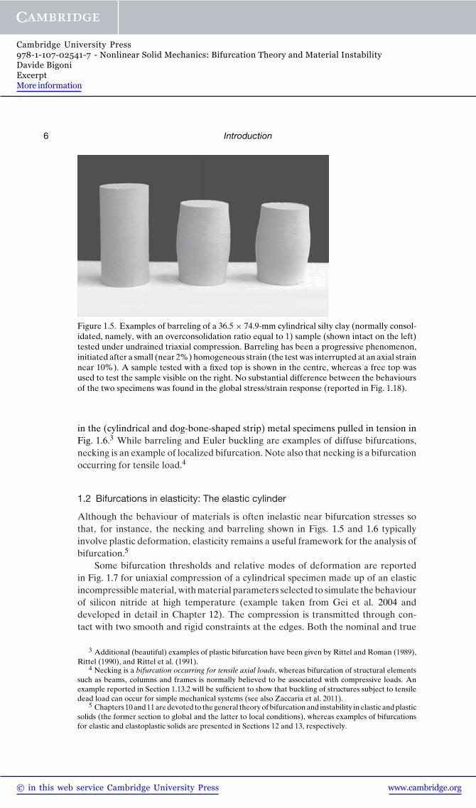
Figure 1.5. Examples of barreling of a 36.5 × 74.9-mm cylindrical silty clay (normally consol-idated, namely, with an overconsolidation ratio equal to 1) sample (shown intact on the left)tested under undrained triaxial compression. Barreling has been a progressive phenomenon,initiated after a small (near 2%) homogeneous strain (the test was interrupted at an axial strainnear 10%). A sample tested with a fixed top is shown in the centre, whereas a free top wasused to test the sample visible on the right. No substantial difference between the behavioursof the two specimens was found in the global stress/strain response (reported in Fig. 1.18).

in the (cylindrical and dog-bone-shaped strip) metal specimens pulled in tension inFig. 1.6.3 While barreling and Euler buckling are examples of diffuse bifurcations,necking is an example of localized bifurcation. Note also that necking is a bifurcationoccurring for tensile load.4

1.2 Bifurcations in elasticity: The elastic cylinder

Although the behaviour of materials is often inelastic near bifurcation stresses sothat, for instance, the necking and barreling shown in Figs. 1.5 and 1.6 typicallyinvolve plastic deformation, elasticity remains a useful framework for the analysis ofbifurcation.5

Some bifurcation thresholds and relative modes of deformation are reportedin Fig. 1.7 for uniaxial compression of a cylindrical specimen made up of an elasticincompressible material, with material parameters selected to simulate the behaviourof silicon nitride at high temperature (example taken from Gei et al. 2004 anddeveloped in detail in Chapter 12). The compression is transmitted through con-tact with two smooth and rigid constraints at the edges. Both the nominal and true

3 Additional (beautiful) examples of plastic bifurcation have been given by Rittel and Roman (1989),Rittel (1990), and Rittel et al. (1991).

4 Necking is a bifurcation occurring for tensile axial loads, whereas bifurcation of structural elementssuch as beams, columns and frames is normally believed to be associated with compressive loads. Anexample reported in Section 1.13.2 will be sufficient to show that buckling of structures subject to tensiledead load can occur for simple mechanical systems (see also Zaccaria et al. 2011).

5 Chapters 10 and 11 are devoted to the general theory of bifurcation and instability in elastic and plasticsolids (the former section to global and the latter to local conditions), whereas examples of bifurcationsfor elastic and elastoplastic solids are presented in Sections 12 and 13, respectively.






1.2 Bifurcations in elasticity: The elastic cylinder 7

Figure 1.6. Examples of localization of deformation occurring for tensile loads in low-carbonsteel samples. Top: Necking is the first mode occurring in the dog-bone-shaped strip shownin the figure. Later, shear banding (with a 45◦ inclination) develops within the necked zone,which eventually degenerates into a fracture (visible in the photo). Bottom: Necking in acylindrical bar under tension.

2000 h/d = 5/2

h/d = 4/2

h/d = 2/2

h/d = 1/2

nominal shear banding

true

surface instability

crit. mode h/d = 1/2




0 0.02 0.04 0.06 0.08 0.1|ε| (–)

|σ|,

|s| (

MPa

)

1800

1600

1400

1200

1000

800

600

400

200

0

Figure 1.7. Bifurcation thresholds (in terms of true σ and nominal s stress versus axial log-arithmic strain) of an elastic, incompressible cylinder uniaxially compressed through smoothand rigid constraints (adapted from Gei et al. 2004). Some modes associated with initial bifur-cations for different aspect ratios (h/d= 1/2,1,2,5/2) are sketched in the upper part. Note thatsurface bifurcation (or surface instability) and shear banding are extreme forms of instability,occurring ‘far’ in the softening regime.






8 Introduction

stresses are reported (the latter dashed) in the figure versus the (absolute valueof) logarithmic strain for homogeneous response. The threshold stresses for thefirst bifurcations are called ‘critical’ (denoted with ‘crit’) and may occur for differ-ent aspect ratios (namely h/d = 1/2, 1, 2, 5/2). These are marked on the curves inFig. 1.7.

The different modes of bifurcation may be triggered by boundary conditions,for instance, if the elastic cylinder represents a specimen in a testing machine, bythe specific test geometry, stiffness of the machine, or friction at the contact withthe loading plates. For example, a high slenderness will induce a Euler-type bifur-cation, whereas friction at the contact between specimen and end supports willfavour development of barreling. The example of the elastic cylinder illustratesthe great variety of bifurcation mechanisms often observable during mechanicaltests.

Two peculiar bifurcation instabilities in Fig. 1.7 will receive a strong attentionlater, namely, surface bifurcation or surface instability and shear banding.6 Theseinstabilities occur at high strain, after other bifurcations, so these represent extremeforms of instabilities.

1.3 Bifurcations in elastoplasticity: The Shanley model

Bifurcation and instability theory is much simpler for elastic materials than forelastoplastic materials. The complication inherent to elastoplastic models, which aredissipative, already can be appreciated by considering the behaviour of the elasto-plastic spring shown in Fig. 1.8 on the left. In particular, since during elastoplasticbehaviour the response differs from loading (stiffness kt , the so-called plastic branchof the constitutive equation) to unloading (stiffness ke, the so-called elastic branch ofthe constitutive equation), the constitutive equation has to relate incremental (insteadof finite, as in elasticity) quantities and in an incrementally non-linear (piece-wise lin-ear) relation (instead of an incrementally linear way, as in nonlinear elasticity). Thecomplication introduced by the constitutive equation yields peculiar features forproblems of plastic bifurcation and instability that can be illustrated with the simpleexample of the celebrated Shanley (1947) model for plastic column buckling. TheShanley model is shown in Fig. 1.8 (centre and right) and consists in a T-shaped rigidrod constrained to move vertically and possibly rotate about the node of the T (seealso Hutchinson 1973, 1974). The rigid rod is connected to two elastoplastic springs(behaving as in Fig. 1.8, left), subject to a vertical compressive load F (taken posi-tive for compression), which before bifurcation is simply equal to P/2. We assumethat F is (1) either at yielding, namely, at its maximum value Fmax (in the plasticbranch of the constitutive equation of the springs; Fig. 1.8, left) or (2) is unload-ing after having reached Fmax. Therefore, the two springs obey the following force

6 Surface instability is characterized by the fact that the wavelengths of the bifurcation mode maybecome infinitely small. This is a tendency already visible in Fig. 12.17 of Chapter 12, where modes R, T andU correspond to increasing circumferential and longitudinal wavenumbers (see Fig. 12.18). Subsequentbifurcations involve smaller wavelengths, which approach zero at surface instability, representing anaccumulation point for bifurcation loads.






1.3 Bifurcations in elastoplasticity: The Shanley model 9

PP

l

b

u

ϑ

Force F

displacement δ

kt kt kt ktke

Fe Ft

ke

unloading

loading

Fmax

F = ktδ

δ

δ

F = keδ

loading

unloading

Figure 1.8. Left: Force-displacement relation for an elastoplastic spring. Centre and right:Shanley model for plastic column buckling. The rigid T-shaped rod has two degrees of freedom{u,θ} and is constrained by two elastoplastic springs, displaying the piecewise-linear force-displacement behaviour shown on the left.

F – displacement δ rate constitutive relation:

1. At yielding: F = Fmax =⇒{

F = kt δ, for plastic loading F > 0,

F = keδ, for elastic unloading F < 0,

2. Within the elastic range: F < Fmax =⇒ F = keδ.

(1.1)

where superposed dots denote rates.

Note the incremental non-linearity (more precisely, piecewise linearity) of the constitutiveequations, which exhibit two different branches, one for plastic loading and another forelastic unloading (the so-called neutral loading corresponds to δ = F = 0). Thisnonlinearity in the rate represents the main complication of elastoplasticity.

It is assumed that the system is loaded until the springs are in the plastic range,without any prior elastic instability. This loading occurs without any rotation anddefines the fundamental path, where F =P/2. Bifurcations are sought as quasi-static(namely, involving negligible dynamical effects) departures from this configuration,in terms of a rate vertical displacement u of the centre of the T-shaped rod and a raterotation θ . Note that we intend with ‘rate’ the derivative with respect to an increasingtime-like parameter governing the loading of the system.

Equilibrium written for a configuration displaced a finite amount u and θ isreadily obtained as

P = Fe +Ft Pl sinθ + (Fe −Ft)bcosθ = 0, (1.2)

with displacements in the springs

ut = u+bsinθ ue = u−bsinθ . (1.3)






10 Introduction

By approximating Eqs. (1.2) and (1.3) for small θ and taking the rates, we obtainthe rate equations, holding for a configuration close to the fundamental path

P = Fe + Ft (Pθ)· l + (Fe − Ft)b = 0, (1.4)

whereas the rate of displacements in the springs are

ut = u+b θ ue = u−b θ , (1.5)

so the constitutive equations of the springs (1.1) allow us to obtain

(Pθ)· = −ke −kt

ke +kt

blP+PRθ u = P

ke +kt+ ke −kt

ke +ktb θ , (1.6)

where

PR = 4(kekt)b2

(ke +kt) l> 0, (1.7)

is the so-called reduced-modulus load. Equations (1.6) are valid if the appropriateloading/unloading conditions are satisfied. For positive (clockwise) θ and using Eqs.(1.5), these conditions are

u−b θ < 0, u+b θ > 0. (1.8)

From Eqs. (1.6) we can observe the following.

• Analysis of bifurcations emanating from the fundamental path, θ = 0, is governedby the equations

ke −kt

ke +kt

blP = (PR −P) θ u = P

ke +kt+ ke −kt

ke +ktb θ . (1.9)

Working Eqs. (1.9) into Eqs. (1.8), we can write the conditions enforcing thesatisfaction of loading/unloading constraints in the springs

PT ≤ P ≤ PE PT = 2ktb2

lPE = 2keb2

l, (1.10)

where PT is the so-called tangent modulus load, whereas PE is the critical loadcorresponding to a purely elastic bifurcation.

For a value of the load P belonging to the interval [PT ,PE], bifurcations arepossible because Eqs. (1.9) always admit a non-trivial solution. There are threeparticular cases of interest: (1) When P = PT , bifurcation occurs as if the twosprings were elastic and both are characterized by a stiffness kt ; moreover, neu-tral loading (i.e., ue = 0) occurs for the unloading spring, which remains ‘frozen’at bifurcation. (2) When P = PR, bifurcation occurs at a fixed load (i.e., forP = 0). (3) When P = PE, a purely elastic bifurcation occurs.

• Integration of the rate Eqs. (1.6) is simple if the springs do not change theirbehaviour. Performing the integration from an initial state where the load isPbif ∈ [PT ,PE] and θ = 0 to a final state in which the load is P = Pbif +�P andthe rotation is θ , we obtain

�P+Pbif

PR= Pbif/PR(PE/PT − 1)+ (PE/PT + 1)l/bθ

(PE/PT − 1)+ (PE/PT + 1)l/bθ, (1.11)




1 introduction - cambridge university...

Documents