1 introduction - arizona state...

Notes on Lidar interpolation

J Ramon Arrowsmithwith contributions from Chris Crosby and Jeff Conner

Department of Geological SciencesArizona State University

Tempe, AZ, [email protected]

May 24, 2006

1 Introduction

Representation of the earth’s surface as a point cloud (xi, yi, zi, where x and y are the horizonal coordinateaxes, z is the vertical, and i is the index of the point) is often done using Light Distance And Ranging(LiDAR) technology from the air or ground (a general reference for much of what follows is El-Sheimy, et al.,2005). This technology uses a scanning laser from a known position to measure the relative distance to thetarget (earth’s surface in our case). The position and orientation of the scanner are estimated using GlobalPositioning System (GPS) and Inertial Measuring Units (IMU; if airborne or vehicle-mounted). Given laserpulse rates at > 10s of khz, these datasets are typically voluminous (>10s of millions of points). In addition,the scattered points are scattered irregularly across the target surface, including the ground, structures, andvegetative canopy.

Given these large data volumes, and typical visualization and analysis methods in earth science, we com-monly make at least 3 assumptions about the surface of interest: 1) it is continuous, 2) z is a single-valuedfunction of x and y (“2.5 dimensional”), and 3) it can be represented by elevations estimated on a regular XY

grid.The purpose of this note is to define the basic geometry of the point cloud and its 2.5D representation on

a grid using local interpolation methods.

2 Geometry of the point cloud

For our purposes, we do not consider the precision or accuracy of the point cloud measurements (typically onthe order of cm to dm for airborne surveys, e.g., El-Sheimy, et al., 2005, p. 46). We also assume that the datacover a small enough area that a universal transverse mercator (UTM) or state plane projection can be usedin a cartesian sense (the horizontal scale is constant). Figure 1 shows a perspective and map view of the pointcloud and the coordinate system and spacing of the regularly spaced nodes or grid (with locations XY ) ontowhich we estimate the elevations Z. The grid nodes are separated by ∆x and ∆y.

3 Surface interpolation (also known as gridding)

Interpolation is the general process of estimating the elevation at a specified grid node from measurementsat surrounding point locations (sample or reference points; El-Sheimy, et al., 2005, Chapter 4). Globalinterpolation methods use all of the known elevations at the reference points to estimate the unknown elevationat the reference point. Example global methods are: Trend surface analysis, Fourier analysis, and Kriging.Given that topographic measurements are not dependent on measurements made a long distance away, analternative and appropriate set of interpolation methods are local. They utilize the elevation information onlyfrom local reference points. El-Sheimy, et al., 2005 delineate the following general implementation for a localinterpolation technique:

1. Define a search area (neighborhood) around the point to be interpolated;

Notes on Lidar interpolation 2

2. Identify (find) the reference points in that neighborhood;

3. Choose a mathematical model to represent the elevation variation over the neighborhood;

4. Use that model to estimate the elevation at the specified grid node.

They also identify a number of local interpolation methods: linear, bilinear, polynomial, nearest neighbor,cubic convolution, moving average, and inverse distance weighting (IDW).

0

100

200

300

0

100

200

300

100

120

140

160

180

200

220

240

260

280

x, Easting (ft)y, Northing (ft)

z, e

leva

tion (

ft)

0 50 100 150 200 250

100

50

0

50

100

150

200

250

300

350

400

x, Easting (ft)

y, N

ort

hin

g (

ft)

points and nodesA B

∆y

∆x

Figure 1: Geometry of LiDAR point cloud (2000 points). A) Perspective view of sample dataset from northernSan Andreas Fault dataset (Harding, et al.). View is to the northeast up a small trough. Note trees on bothsides of the drainage. B) Map view of point cloud (black dots) with regularly spaced nodes (grid, red crosses)separated by ∆x and ∆y. Coordinate system is x, y, z or Easting, Northing, Elevation. These data are in feet.


4 Local interpolation algorithms

In the following algorithm, we load the data, define the grid and neighborhoods, find the points, and interpolateusing 4 estimation methods (minimum, maximum, mean, and weighted mean–points are inversely weightedby their distance from the grid node).

1. Load points

2. Define variables:∆x and ∆y–grid spacing in x and ySearch radius–radius of neighborhood from grid node

3. Compute variables:From point cloud x and y ranges, determine xmin, xmax, ymin, ymax.Compute node locations Xj,kYj,k by incrementing ∆x from xmin not to exceed xmax; ditto for y. j, k

are the X and Y indices respectively.

4. Find all points in neighborhood: dj,k ≤√

(xi − Xj,k)2 + (yi − Yj,k)2. Where dj,k is the horizontaldistance between the ith point and the j, k node. Note that this is the most computationally challengingpart of the task, given that the data are unsorted. A naive implementation (such as that I present below)searches the entire dataset each time. Typical implementations use a quadtree approach to presort thedata into local areas for computation. Some overlap is necessary between adjacent quadtree nodes toensure that all the points in the neighborhood of a grid node are found. See Appendix 2 for variousquadtree pseudocodes. Given the point density for LiDAR, dj,k ≤

√2∆x will find all of the points in

the circle that circumscribes the grid cell.

5. Estimate elevation Zj,k at Xj,kYj,k:

Zmin = min(Zl) (1)

Zmean = mean(Zl) (2)

Zmax = max(Zl) (3)

ZIDW =

∑n

l=1

Zl

dp

l∑n

l=1

1

dp

l

(4)

where l is the index of the points in neighborhood, and p is the weight (typically 2). ZIDW is InverseDistance Weighting from El-Shiemy, et al., 2005. If no points are within the search radius, set Zj,k =NaN . Note that the Zmin and Zmax computations could be implemented with the IDW approach.

I implemented the above algorithm in Matlab (see Appendix 1).

5 Examples

Figure 2 illustrates a case of local interpolation of the 2000 points in Figure 1 from the Northern San AndreasFault dataset. Because the search radius is less than the grid spacing, the neighborhoods for local interpolationaround each grid point are clear. Some LiDAR datasets (such as this one, are classified by return type (ground,vegetation, structure, blunder). From a query by classification, one can compute a bare earth DEM or a canopytop DEM. In my computations, Zmin is a crude way to estimate the bare earth without the classification.Similarly, the Zmax is a local estimate of canopy top, and the Zdif = Zmax−Zmin estimates the canopy heightover the search radius assuming that the topography does not change significantly relative to canopy. Notesmall differences between Zmean and ZIDW . Here, p = 2, and so the weighted mean of ZIDW emphasizes localpoints much more than the straight average of Zmean.


0 100 2000

50

100

150

200

250

Easting (ft)

Nort

hin

g (

ft)

points and nodes

0 100 2000

50

100

150

200

250

Zmax

0 100 2000

50

100

150

200

250

Zmin

0 100 2000

50

100

150

200

250

Zmean

0 100 2000

50

100

150

200

250

Zidw

0

50

100

150

200

250

0 100 2000

50

100

150

200

250

Zdif

Figure 2: First example of local interpolation. Upper left plot shows point cloud in black with grid nodes andsurrounding neighborhood points used in local interpolation in magenta. Zmin, Zmax, Zmean all are computedwith equal weights on points in neighborhood, while ZIDW inversely weights the contributions of the points bytheir distance. At lower left, Zdif is the difference between the Zmin and Zmax. It is a measure of the canopyheight that is independent of the point classifications that may be made for ground and vegetation. Thecolorbar at right applies to the elevation range for all of the plots. p = 2, ∆x = ∆y = 50ft, and dj,k ≤ 20ft.

Figure 3 illustrates the second example of local interpolation on this dataset. The grid spacing is stillfairly coarse at 25 ft, and the search radius is 35.4 ft. The result is a smoothed representation of the localtopography and canopy. Zdif shows the smoothed canopy height.

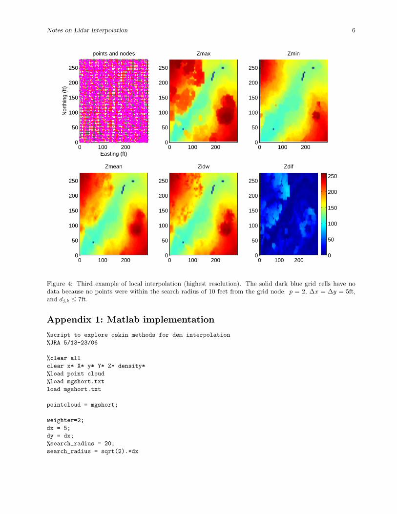
Figure 4 illustrates the third example of local interpolation on this dataset. I have produced a highresolution DEM with ∆x = ∆y = 5ft, and di = 7ft. One can see the finer textures of the canopy in Zmax andZdif . Zmin is fairly smooth mostly ground surface while the Zmean and Zidw obviously are a representationof the surface that includes both the ground and the vegetation.

Point densities per pixel for the three examples are presented in Figure 5. The left plot shows pointdensities up to about 55 pixel−1 with dj,k ≤ 20ft (Figure 2). Figure 3’s point densities (middle) are as highas 168 pixel−1 with dj,k ≤ 35.4ft. For the high resolution gridding shown in Figure 4, point densities rangebetween 0 and 12 pixel−1 for dj,k ≤ 7ft (Figure 5 right).


0 100 2000

50

100

150

200

250

Easting (ft)

Nort

hin

g (

ft)

points and nodes

0 100 2000

50

100

150

200

250

Zmax

0 100 2000

50

100

150

200

250

Zmin

0 100 2000

50

100

150

200

250

Zmean

0 100 2000

50

100

150

200

250

Zidw

0

50

100

150

200

250

0 100 2000

50

100

150

200

250

Zdif

Figure 3: Second example of local interpolation. p = 2, ∆x = ∆y = 25ft, and dj,k ≤ 35.4ft.

6 References

El-Sheimy, N, Valeo, C., and Habib, A., 2005, Digital terrain modeling: acquisition, manipulation, and appli-

cations, Artech House: Boston, MA, 257 pp.


0 100 2000

50

100

150

200

250

Easting (ft)

Nor

thin

g (f

t)

points and nodes

0 100 2000

50

100

150

200

250

Zmax

0 100 2000

50

100

150

200

250

Zmin

0 100 2000

50

100

150

200

250

Zmean

0 100 2000

50

100

150

200

250

Zidw

0

50

100

150

200

250

0 100 2000

50

100

150

200

250

Zdif

Figure 4: Third example of local interpolation (highest resolution). The solid dark blue grid cells have nodata because no points were within the search radius of 10 feet from the grid node. p = 2, ∆x = ∆y = 5ft,and dj,k ≤ 7ft.

Appendix 1: Matlab implementation

%script to explore oskin methods for dem interpolation

%JRA 5/13-23/06

%clear all

clear x* X* y* Y* Z* density*

%load point cloud

%load mgshort.txt

load mgshort.txt

pointcloud = mgshort;

weighter=2;

dx = 5;

dy = dx;

%search_radius = 20;

search_radius = sqrt(2).*dx


20

25

30

35

40

45

50

0 100 2000

50

100

150

200

250

Easting (ft)

Nort

hin

g (

ft)

point density per pixel

60

80

100

120

140

160

0 100 2000

50

100

150

200

250

2

4

6

8

10

12

0 100 2000

50

100

150

200

250

Figure 5: Point densities per pixel for the three examples presented here. Figure 2’s density is shown in theleft plot; Figure 3’s density is in the middle, and Figure 4’s density is on the right.

x = pointcloud(:,1)-min(pointcloud(:,1));

y = pointcloud(:,2)-min(pointcloud(:,2));

z = pointcloud(:,3);

minx = min(x);

maxx = max(x);

miny = min(y);

maxy = max(y);

minz = min(z);

maxz = max(z);

xx = (minx+dx):dx:(maxx);

yy = (miny+dy):dy:(maxy);

[X,Y] = meshgrid(xx,yy’);

figure(1)

clf


subplot(2,3,1)

plot(x,y, ’k.’)

hold on

plot(X, Y, ’r+’)

xlabel(’Easting (ft)’)

ylabel(’Northing (ft)’)

for j=1:length(yy)

for k=1:length(xx)

%plot(X(j,k), Y(j,k), ’bo’)

%Use this to search only on those points within the actual grid cell (within dx and dy of the node)

%tf = x<= X(j,k)+dx./2 & x>=X(j,k)-dx./2 & y<=Y(j,k)+dy./2 & y>=Y(j,k)-dy./2;

%locs=find(tf);

%if length(locs)==0

% Zmin(j,k)=NaN;

% Zmean(j,k)=NaN;

% Zmax(j,k)=NaN;

%else

% Zmin(j,k)=min(z(locs));

% Zmean(j,k)=mean(z(locs));

% Zmax(j,k)=max(z(locs));

%end

tf = x<= X(j,k)+search_radius & x>=X(j,k)-search_radius

& y<=Y(j,k)+search_radius & y>=Y(j,k)-search_radius;

locs=find(tf);

localx = x(locs);

localy = y(locs);

localz = z(locs);

dist = sqrt((localx-X(j,k)).^2 + (localy-Y(j,k)).^2);

locs_radius=find(dist<=search_radius);

plot(localx(locs_radius), localy(locs_radius), ’m.’)

axis([minx maxx miny maxy])

title(’points and nodes’)

if length(locs_radius)==0

Zmin(j,k)=NaN;

Zmean(j,k)=NaN;

Zmax(j,k)=NaN;

densitymap(j,k)=NaN;

else

Zmin(j,k)=min(localz(locs_radius));

Zmean(j,k)=mean(localz(locs_radius));

Zmax(j,k)=max(localz(locs_radius));

Zidw(j,k) = sum(localz./(dist.^weighter))./sum(1./(dist.^weighter));

densitymap(j,k)=length(localz);


end

end

end

clims = [0 260];

subplot(2,3,2)

plot(minx, miny, ’k.’)

hold on

imagesc(xx’, yy, Zmax, clims)

axis([minx maxx miny maxy minz maxz])

%colorbar

title(’Zmax’)

subplot(2,3,3)


hold on

imagesc(xx’, yy, Zmin, clims)


%colorbar

title(’Zmin’)

subplot(2,3,4)


hold on

imagesc(xx’, yy, Zmean, clims)


%colorbar

title(’Zmean’)

subplot(2,3,5)


hold on

imagesc(xx’, yy, Zidw, clims)


%colorbar

title(’Zidw’)

subplot(2,3,6)


hold on

imagesc(xx’, yy, Zmax-Zmin, clims)


colorbar

title(’Zdif’)

figure(2)

clf

surfl(X,Y,Zmax)

shading interp


hold on

surfl(X,Y,Zmin)

colormap(jet)



zlabel(’Elevation (ft)’)

figure(3)

clf


hold on

imagesc(xx’, yy, densitymap)

axis([minx maxx miny maxy])

colormap cool

colorbar



title(’point density per pixel’)

Psuedo code for Quadtree implementation by Jeff Conner

1st Try (Brute force)

Searches the input file in its entirety for every grid point. Works ok on small data sets.

For all Xi in Xj,k

For all Yi in Yj,k

Djk = sqrt( (Xi - Xjk)^2 (Yi - Yjk)^2)

For all Djk in input file <= radius

Zi = average(Djk

2nd try (Quad Tree Method)

Faster than 1st try but runs out of memory on larger data sets. Everything is stored in memory. Trying to fixwith temp files.

BuildTree(treeptr, depth)

If depth is not 0

If child node is null

Create new boundary node

Depth = depth - 1

BuildTree(child node, depth)

Else

If next node is not null

BuildTree(next node, depth)

Else

Depth = Depth + 1

BuildTree(parent_node->next_node, depth


Insert(treeptr, xi, yi, radius)

If point is within node boundary

Is node a bounding node

If node has child nodes

Insert(child node, xi, yi, radius)

Else

Create point node

Else


Insert(next node, xi, yi, radius)

Else

Create new point on next node

Else


Insert(next node, xi, yi, radius)

Plot(treeptr, Xi, Yi, radius)

If xy is within current node bounds

If node is "bounding" node

If node.childnode is not null

plot(childnode, Xi, Yi, radius)

Else

While tree node is not false


For all Djk <= radius

Zi = average(Djk

Else not in bounding area

If next node is not false

Plot(next node, Xi, Yi, radius

Main

BuildTree(tree, depth)

For all points x,y in input file

Insert(tree, x, y, depth)

For all Xi in Xj,k

For all Yi in Yj,k

Plot(tree, gridXstart + (Xi * resolution), gridYstart + (Yi * resolution), radius)

3rd try (Database method)

Attempts to unload query times to a mysql database. Faster than 1st try but slower than second. Also failson large datasets with out of memory errors.

For all points in input file

Insert points into data base

For all Xi in Xj,k

For all Yi in Yj,k


For all points in database where Djk <= radius

Zi = average(Djk)


Sample SQL Commmand

SELECT * FROM (SELECT SQRT( ((6197211.71 - point.x) * (6197211.71 - point.x)) +

((1964738.78 - point.y)* (1964738.78 - point.y)) )

as d,z FROM point)AS dis WHERE d < 100.0 ORDER BY z

SQL statement code in java:

xval = xmin + (x * res);

yval = ymin + (y * res);

xmin is the starting x coordinate for the region

ymin is the starting y coordinate for the region

res is the resolution of the grid

x and y are the corresponding current positions in the grid

SQL query statement java passes to the database

query2 = "SELECT * FROM (SELECT SQRT( (("+xval+" - point.x) * ("+xval+" - point.x)) +"+

"(("+yval+" - point.y)* ("+yval+" - point.y)) )as d,z "+

"FROM point)AS dis "+

"WHERE d < "+radius+" "+

"ORDER BY z ";

query_results = new ArrayList();

query_results = db.DBQueryRelation(query2, "z", connection);

Database has a single table called "point" with 3 columns x, y and z

1 introduction - arizona state...

Documents