Complex Variables020701 F. Porter

Revision 130411

1 Introduction

This note is intended as a review and reference for the basic theory of complexvariables. For further material, and more rigor, Whittaker and Watson isrecommended, though there are very many sources available, including abrief review appendix in Matthews and Walker.

2 Complex Numbers

Let z be a complex number, which may be written in the forms:

z = x+ iy (1)

= reiθ, (2)

where x, y, r, and θ are real numbers. The quantities x and y are referredto as the real and imaginary parts of z, respectively:

x = <(z), (3)

y = =(z). (4)

The quantity r is referred to as the modulus or absolute value of z,

r = |z| =√x2 + y2, (5)

and θ is called the argument, θ = arg(z), or the phase, or simply the angleof z. We have the transformation between these two representations:

x = r cos θ, (6)

y = r sin θ, (7)

and finally alsoθ = tan−1(y/x), (8)

with due attention to quadrant. Noticing that eiθ = ei(θ+2nπ), where n is anyinteger, we say that the principal value of arg z is in the range:

−π < arg z ≤ π. (9)

1

y

x

r

z

z*

θ

θ−

Figure 1: Complex number and its complex conjugate.

The complex conjugate, z∗, of z is obtained from z by changing thesign of the imaginary part:

z∗ = x− iy = re−iθ. (10)

The product of two complex numbers, z1 and z2, is given by:

z1z2 = r1eiθ1r2e

iθ2 = r1r2ei(θ1+θ2)

= (x1 + iy1)(x2 + iy2) = (x1x2 − y1y2) + i(x1y2 + x2y1). (11)

Notice thatzz∗ = x2 + y2 = |z|2. (12)

It is also interesting to notice that in the product:

z1z∗2 = (x1x2 + y1y2)− i(x1y2 − x2y1), (13)

the real part looks something like a “scalar product” of two vectors, and theimaginary part resembles a “cross product”.

3 Complex Functions of a Complex Variable

We are interested in (complex-valued) functions of a complex variable z. Inparticular, we are especially interested in functions which are single-valued,continuous, and possess a derivative in some region.

2

Defining a suitable derivative requires some care. Start with the definitionfor real functions of a real number:

f ′(x) =df

dx(x) = lim

∆x→0

f(x+ ∆x)− f(x)

∆x. (14)

But in the complex case we have real and imaginary parts to worry about.First, define what we mean by a limit. Let f(z) be a single-valued functiondefined at all points in a neighborhood of z0 (except possibly at z0). Thenwe say that f(z) → w0 as z → z0, or limz→z0 f(z) = w0, if, for every ε > 0,there exists a δ > 0 such that (Fig. 2):

|f(z)− w0| < ε ∀z satisfying 0 < |z − z0| < δ. (15)

Note that we have not required “f(z0)” to be defined, in order to define thelimit (Fig. 3).

y

x

z 0

d

Figure 2: Circle of radius δ about z0.

"f(z)"

"z"z 0

Figure 3: Function not defined at z0.

However, in order to define the derivative at z0, we require f(z0) to bedefined. If limz→z0 = f(z0), where the limit exists, then we say that f(z) iscontinuous at z0. In general f(z) is complex, and we may write:

f(z) = u(x, y) + iv(x, y), (16)

3

where u and v are real. Then limz→z0 = f(z0) implies

limx→x0, y→y0

u(x, y) = u(x0, y0), (17)

limx→x0, y→y0

v(x, y) = v(x0, y0), (18)

where the path of approach to the limit point must lie within the region ofdefinition. We may thus define continuity to the boundary of a closed region,if the path is within the region.

Now, in our definition of f ′(z), we note that there are an infinite numberof possible paths along which we can make ∆z = ∆x+ i∆y → 0.

y

x

Figure 4: Various paths along which to approach a point.

For our derivative to be well-defined, we demand that the value of f ′(z)be independent of the way in which ∆z → 0. Thus, if we approach along thepath ∆x = 0:

f ′(z) = lim∆y→0

f(z + i∆y)− f(z)

i∆y

= lim∆y→0

{u(x, y + ∆y)− u(x, y)

i∆y+i [v(x, y + ∆y)− v(x, y)]

i∆y

}

= −i∂u∂y

+∂v

∂y. (19)

If instead we make our approach along the path ∆y = 0, we obtain:

f ′(z) = lim∆x→0

f(z + ∆x)− f(z)

∆x

=∂u

∂x+ i

∂v

∂x(20)

4

The two expressions are equal if and only if the real and imaginary parts areseparately equal:

∂u

∂x=

∂v

∂y(21)

∂u

∂y= −∂v

∂x. (22)

These important conditions are known as the Cauchy Riemann equations,or C-R equations, for short. We may state this in the following theorem:

Theorem: If u, v possess first derivatives throughout a neighborhood of z0,which are continuous at z0, then the Cauchy Riemann equations, ifsatisfied, guarantee the existence of df

dz(z0).

Proof: Write:

∆u =∂u

∂x∆x+

∂u

∂y∆y + εux∆x+ εuy∆y (23)

∆v =∂v

∂x∆x+

∂v

∂y∆y + εvx∆x+ εvy∆y, (24)

where the correction terms for non-linearities, εij, approach zero as∆x,∆y → 0.

Using the Cauchy Riemann equations, we obtain:

∆u =∂u

∂x∆x− ∂v

∂x∆y + εux∆x+ εuy∆y (25)

∆v =∂v

∂x∆x+

∂u

∂x∆y + εvx∆x+ εvy∆y. (26)

Thus,

∆f

∆z=

∆u+ i∆v

∆z

=∂u∂x

(∆x+ i∆y) + i ∂v∂x

(∆x+ i∆y) + εx∆x+ εy∆y

∆x+ i∆y, (27)

where εx ≡ εux + iεvx → 0, εy ≡ εuy + iεvy → 0 as ∆x,∆y → 0.Furthermore, ∣∣∣∣∣ ∆x

∆x+ i∆y

∣∣∣∣∣ ≤ 1,

∣∣∣∣∣ ∆y

∆x+ i∆y

∣∣∣∣∣ ≤ 1. (28)

Therefore,df

dz= lim

∆z→0

∆u+ i∆v

∆z=∂u

∂x+ i

∂v

∂x, (29)

independent of path. This completes the proof.

5

We have the following equivalent ways of expressing the derivative:

df

dz=∂u

∂x+ i

∂v

∂x=∂v

∂y+ i

∂v

∂x=∂v

∂y− i∂u

∂y=∂u

∂x− i∂u

∂y. (30)

It is of interest to also consider this discussion in terms of the polar form.In this case, we may consider the ∆r = 0 path:

y

x

z

q

Dq

Dz D

z

z+

Figure 5: Polar path description.

f ′(z) = lim∆θ→0

f(zei∆θ)− f(z)

z(ei∆θ − 1)

= lim∆θ→0

{u(r, θ + ∆θ)− u(r, θ)

iz∆θ+i [v(r, θ + ∆θ)− v(r, θ)]

iz∆θ

}

= − iz

∂u

∂θ+

1

z

∂v

∂θ. (31)

Similarly, for the ∆θ = 0 path:

f ′(z) = lim∆r→0

f[(r + ∆r)eiθ

]− f(z)

eiθ∆r

= lim∆r→0

{u(r + ∆r, θ)− u(r, θ)

eiθ∆r+i [v(r + ∆r, θ)− v(r, θ)]

eiθ∆r

}

=1

eiθ∂u

∂r+

i

eiθ∂v

∂r. (32)

Hence,

eiθf ′(z) =∂u

∂r+ i

∂v

∂r= − i

r

∂u

∂θ+

1

r

∂v

∂θ. (33)

We have thus obtained the Cauchy-Riemann relations in polar form:

∂u

∂r=

1

r

∂v

∂θ(34)

∂v

∂r= −1

r

∂u

∂θ. (35)

6

A function f(z) of complex variable z is called analytic at the point z0 ifit is single-valued and possesses a derivative at every point in a neighborhoodof z0. Otherwise, z0 is a singular point of f(z). If f(z) is analytic at everypoint in a simply connected open region (“domain”) D, then it is referredto as analytic throughout D. Other terms that are often used for this (withsome variation of meaning) are regular and holomorphic. Sometimes theterm “analytic” is not required to be single-valued, that is, single-valuednessin a domain D means that, after following any closed path in D, the functionf(z) returns to its initial value. If f(z) is analytic for all finite z, then f(z)is an entire function.

Examples:

• f(z) = z3 is an entire function.

• f(z) = 1/z2 is analytic everywhere except at z = 0, where it is notdefined. We note that for this function,

u =x2 − y2

(x2 + y2)2, v = − 2xy

(x2 + y2)2. (36)

• f(z) = z3/2 is analytic everywhere except at z = 0. Let’s look at whythis is the case in some detail. We may write

z3/2 = r3/2e3iθ/2 = r3/2(cos 3θ/2 + i sin 3θ/2). (37)

Hence,

∂u

∂r=

3

2r1/2 cos 3θ/2 (38)

∂v

∂r=

3

2r1/2 sin 3θ/2 (39)

1

r

∂u

∂θ= −3

2r1/2 sin 3θ/2 (40)

1

r

∂v

∂θ=

3

2r1/2 cos 3θ/2. (41)

Comparison with Eqns. 34 and 35 shows that the C-R conditions aresatisfied everywhere. Now consider a path containing the origin as aninterior point (see Fig. 6). We’ll start at z = εei0, with ε real. Table 1shows the values of f(z) as we traverse the path once around the origin.We see that f(z) = z3/2 is multi-valued in any neighborhood of theorigin, and hence is not analytic at z = 0.

7

y

x

e

Figure 6: Circular path around origin, radius ε.

Table 1: Evaluation of the function z3/2 at various points on a circle.

θ z f(z) = z3/2

0 ε ε3/2

π/2 iε ε3/2ei3π/4

π −ε ε3/2ei3π/2 = −iε3/23π/2 −iε ε3/2ei9π/4

2π ε ε3/2ei3π = −ε3/2

4 Riemann Surfaces

Let us continue to think about the interesting f(z) = z3/2 example. Notethat if θ = 4π and r = ε, then z3/2 = ε3/2ei6π = ε3/2, so we come back tothe θ = 0 value after two circuits. Thus z3/2 is a double-valued function. Wemay visualize this behavior via the use of Riemann surfaces, or sheets.For z3/2, we have two sheets (Fig. 7).

The point z = 0 is called a branch point. Since there are only a finitenumber of branches (2) for this function, the origin is called an algebraicbranch point.

For another example, the function f(z) = z1/4 will have four branches,see Table 2 and Fig. 8.

Now consider the function f(z) = ln z, defined by ef(z) = z:

f(z) = ln z = ln r + iθ. (42)

This function has an infinite number of branches. In this case, the pointz = 0 is called a logarithmic branch point.

We note a couple of things about branches:

• There may be many branch points for a function.

8

Figure 7: Two Riemann sheets for the double-valued function z3/2. Thelower sheet is for 0 ≤ θ < 2π, 4π ≤ θ < 6π, etc., and the top sheet is for2π ≤ θ < 4π, etc. The branch cuts are indicated by the cuts in the planes.

Table 2: The function f(z) = z1/4, evaluated at multiples of 2π.

θ eiθ/4

0 12π eiπ/2 = i4π eiπ = −16π ei3π/2 = −i8π ei2π = 1

• There are many ways to make branch cuts, but they can only terminateat a branch point, they cannot intersect themselves, and they must havethe same form on all sheets.

For a slightly more complicated example illustrating these ideas, considerthe function:

f(z) =√

1− z2 = (1− z)1/2(1 + z)1/2. (43)

This function has singularities (branch points) at z = ±1. There are twosheets, and various possible ways of choosing the branch cuts, as illustratedin Fig. 9.

There is a choice in how to take branch cuts – one makes cuts that areconvenient to the problem at hand (for example, when we integrate along apath, we arrange it so that the path does not cross a cut). Branch cuts areused in effect to make multi-valued functions “single-valued” – if you don’tcross a branch, you stay on the same sheet.

9

1

2

3

4

0,8π

2π

4π

6π

Sheet

Figure 8: Four Riemann sheets for the quadruple-valued function z1/4. Theview is edge-on, with the branch cut at the transitions among the sheets.

x

y

s s-1 +1 x

y

s s-1 +1 x

y

s s-1 +1

Figure 9: Some possible choices of branch cuts for the function√

1− z2.

5 Integration of Complex Functions

As with the derivative, we must face the problem of forming an integral thatmakes sense in some correspondence with the integral for real functions. Forreal functions, the indefinite integral may be “defined” as the inverse of dif-ferentiation (i.e., as the limit of a sum, rather than the limit of a difference).For a complex function, such an indefinite integral may not always exist.

Consider f(z) = z∗ = x− iy. Suppose

F (z) =∫f(z) dz = U + iV, (44)

and (if integration is inverse of differentiation)

dF

dz= f(z) = x− iy. (45)

If the derivative exists, we must be able to use the Cauchy-Riemann equa-tions, hence,

dF

dz=∂U

∂x− i∂U

∂y= x− iy. (46)

Thus,∂U

∂x= x,

∂U

∂y= y, (47)

10

and∂2U

∂x2+∂2U

∂y2= 2. (48)

Let us see what the Cauchy-Riemann equations imply for this quantity:

∂

∂x

[∂U∂x

=∂V

∂y

](49)

∂

∂y

[∂U∂y

= −∂V∂x

]. (50)

Therefore:∂2U

∂x2+∂2U

∂y2= 0, (51)

which may be recognized as Laplace’s Equation in two dimensions. Thus,F (z) cannot be an analytic function; it does not possess a derivative, andthere exists no function with derivative x− iy. This suggests that we shouldrestrict consideration to functions which are analytic in the region of interest.

Referring to Fig. 10, let us consider the definite integral:∫ β

αf(z)dz. (52)

x

y

α

β

Figure 10: Possible paths of integration from α to β.

There are an infinite number of possible paths to integrate along. In general,we must specify the path, e.g., ∫ β

α

C

f(z) dz. (53)

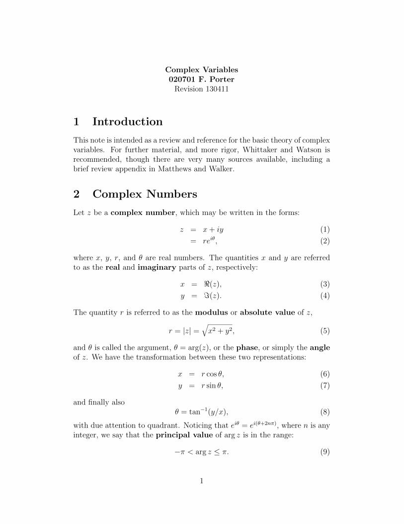
To define this integral, first divide path C into n intervals by pointsz0 = α, z1, z2, . . . , zn = β, as in Fig. 11. Let ∆jz ≡ zj − zj−1, and let z′j be

11

a point on C between zj−1 and zj. Then we define the line integral along Cas: ∫ β

α

C

f(z)dz = limn→∞

n∑j=1

f(z′j)∆jz, (54)

where we require the intervals to satisfy:

limn→∞

nmaxj=1|∆jz| = 0, (55)

and the limit must exist, of course. Note that this definition is compatiblewith the usual definition for real variables.

z j

z j-1

zj'

α

β

=

= z

z0

n

Figure 11: Dividing a path into intervals to obtain an approximate integral.

We list some immediate consequences of our definition:

1. Considering ∆jz → −∆jz, we have the path-reversed integral:∫ α

β

C

f(z)dz = −∫ β

α

C

f(z)dz. (56)

2. If k is any complex constant, then∫ β

α

C

kf(z)dz = k∫ β

α

C

f(z)dz. (57)

3. If the integrals of f and g separately exist, then the integral of theirsum exists, and:∫ β

α

C

[f(z) + g(z)] dz =∫ β

α

C

f(z)dz +∫ β

α

C

g(z)dz. (58)

12

4. If γ is a point on C (between α and β), then∫ γ

α

C

f(z)dz +∫ β

γ

C

f(z)dz =∫ β

α

C

f(z)dz. (59)

Toward proving this, note that we can always arrange our subintervalssuch that γ is a dividing point.

5. If M = maxβαC|f(z)| (including the endpoints) then:

∣∣∣∫ β

α

C

f(z)dz∣∣∣ =

∣∣∣ limn→∞

n∑j=1

f(z′j)∆jz∣∣∣

≤ limn→∞

n∑j=1

∣∣∣f(z′j)∆jz∣∣∣ (follows from triangle inequality)

≤ M∫ β

α

C

|dz| = MLC , (60)

where LC is the length of the integration path (in the usual Euclideansense).

6 Cauchy’s Theorem

If a function f(z) is analytic at all points on and inside a contour C, then∫Cf(z)dz = 0. (61)

Note that by “contour”, we mean a simple closed curve. We could also usethe notation

∮to stress this. Our assertion is known as Cauchy’s Theorem.

Let us prove the theorem: Assume f(z) is analytic as stated. Writef(z) = u(x, y) + iv(x, y). Then:∫

Cf(z) dz =

∫C

(u+ iv)(dx+ idy)

=∫C

(udx− vdy) + i∫C

(udy + vdx) (62)

Let S stand for the region enclosed by contour C. Green’s theorem statesthat, for functions α and β:∫

Cαdx+ βdy =

∫S

(∂β

∂x− ∂α

∂y

)dxdy. (63)

13

CS

Figure 12: Contour and surface of integration in Green’s theorem.

Therefore,∫Cf(z) dz = −

∫S

(∂v

∂x+∂u

∂y

)dxdy + i

∫S

(∂u

∂x− ∂v

∂y

)dxdy

= 0, by the Cauchy-Riemann relations. (64)

Cauchy’s theorem tells us that the integral of an analytic function ispath-independent in a domain of analyticity:∫ β

α Cf(z) dz =

∫ β

α C′f(z) dz

=∫ β

αf(z) dz, (65)

where the latter equality is without ambiguity, due to Cauchy’s theorem.

x

y

α

β

C'

C

Figure 13: Equivalent paths of integration in a region of analyticity.

Note that the way we have stated Cauchy’s theorem, it holds for func-tions which have singularities, provided our contours do not “encircle” thesingularities:

14

C1

C2

(a) (b)

Figure 14: (a)∫C1+C2

f(z) dz = 0, where C2 encircles a singularity, but the“contour” C1 + C2 does not. Integrals along the portions joining C1 and C2

cancel out. (b) A branch cut may be chosen for convenience, so that thecontour does not cross it.

7 Indefinite Integral of an Analytic Function

Let f(z) be analytic in simply connected domain D. Then

F (z) =∫ z

z0f(z′) dz′ (66)

depends only on z and z0 (and not the path), as long as the path is entirelyin D.

What is F ′(z) = dFdz

(z) (for z ∈ D)?

F (z + ∆z)− F (z)

∆z=

1

∆z

[∫ z+∆z

z0f(z′)dz′ −

∫ z

z0f(z′) dz′

]

=1

∆z

∫ z+∆z

zf(z′)dz′

= f(z) +1

∆z

∫ z+∆z

z[f(z′)− f(z)] dz′. (67)

The last integral is path independent in D, so chose for path the straightline segment joining z and z + ∆z (noting that, for ∆z small enough, sucha path must exist). Thus, by the continuity of f(z), given an ε > 0, we canalways find |∆z| small enough such that |f(z′)− f(z)| < ε for any z′ on thepath. Thus, ∣∣∣∣∣

∫ z+∆z

z[f(z′)− f(z)] dz′

∣∣∣∣∣ < ε|∆z|. (68)

Given any ε > 0 then, we can find a ∆z > 0 such that∣∣∣∣∣F (z + ∆z)− F (z)

∆z− f(z)

∣∣∣∣∣ < ε. (69)

15

Therefore,

F ′(z) =d

dz

∫ z

z0f(z′) dz′ = f(z). (70)

The indefinite integral of an analytic function is an analytic function.It is important, when performing integrations, to be careful about sin-

gularities and regions of non-analyticity. For example, consider the integral∫ 1−1

1zdz. We might try an integration path along a semi-circle in the positive

y plane – 1/z is analytic there.

y

y

x x-1 +1

-1 +1

(a) (b)

eiθ

Figure 15: Two possible semi-circular paths from −1 to +1.

We let z = eiθ, and hence dz = ieiθdθ. Alternatively, we could choose tointegrate along a semicircle in the negative y plane – 1/z is analytic there aswell. The two choices yield:

I+ = i∫ 0

πe−iθeiθdθ = −iπ (71)

I− = i∫ 2π

πe−iθeiθdθ = iπ. (72)

The two answers are different! The path-dependence is a result of the factthat we have chosen paths which lie in different simply-connected domainsof analyticity. There is a branch cut from the origin, a singular point. Notethat, while 1/z is not multi-valued, its integral (ln z) is.

8 Cauchy Integral Formula

Suppose f(z) is analytic everywhere in some domain D. Consider the inte-gral: ∫

C

f(z)

z − z0

dz, (73)

16

where C is contained in D, and z0 is interior to C. Thus, f(z)z−z0 is analytic

everywhere on and inside C, except at the point z = z0. The integral isunchanged if we deform the contour to the circle C0 with center at z0:

D

z

CC

0

0

Figure 16: Domain D, contour C and deformed contour C0 about point z0.

∫C

f(z)

z − z0

dz =∫C0

f(z)

z − z0

dz

=∫C0

f(z0)

z − z0

dz +∫C0

f(z)− f(z0)

z − z0

dz. (74)

Consider the second of the two integrals in the above expression:∣∣∣∣∣∫C0

f(z)− f(z0)

z − z0

dz

∣∣∣∣∣ ≤∫C0

|f(z)− f(z0)||z − z0|

|dz|. (75)

Since f(z) is analytic at z0, it must be continuous there. Hence, given anyε > 0, there exists a δ > 0 such that |f(z)− f(z0)| < ε whenever |z− z0| < δ.We pick an ε, and let δ = |z−z0|, i.e., we pick a circle of small enough radiussuch that |f(z) − f(z0)| < ε on the circle. Remember that the value of the

17

integral does not depend on the radius of the circle. Thus,∣∣∣∣∣∫C0

f(z)− f(z0)

z − z0

dz

∣∣∣∣∣ ≤ ε

δ

∫Cδ

|dz|

≤ 2πε. (76)

The integral is smaller than any positive number, i.e., is equal to zero. There-fore, ∫

C0

f(z)

z − z0

dz = f(z0)∫C0

dz

z − z0

= f(z0)∫ 2π

0

ireiθdθ

reiθ(letting z − z0 = reiθ)

= 2πif(z0). (77)

We have derived Cauchy’s Integral Formula: For any function f(z) whichis analytic on and inside the contour C,

f(z0) =1

2πi

∫C

f(z)

z − z0

dz. (78)

Note that the Cauchy integral formula tells us that if we know the value of afunction everywhere along a closed contour, then we know its value at everypoint inside the contour, provided the function is analytic on and inside thecontour.

8.1 Cauchy Integral Formula and Derivatives of an An-alytic Function

Start with Cauchy’s integral formula (assuming f(z) appropriately analytic),and take derivatives:

f(z) =1

2πi

∫C

f(z′)

z′ − zdz′ (79)

df

dz=

1

2πi

∫C

f(z′)

(z′ − z)2dz′ (80)

d2f

dz2=

2

2πi

∫C

f(z′)

(z′ − z)3dz′ (81)

· · ·dnf

dzn=

n!

2πi

∫C

f(z′)

(z′ − z)n+1dz′. (82)

Is this procedure justified? If so, then we have evidently shown that thederivative of an analytic function is analytic, at least at all points inside C.

18

If f(z) is analytic, we know its derivative exists:

f ′(z) = limh→0

f(z + h)− f(z)

h

= limh→0

1

2πih

[∫C

f(z′) dz′

z′ − z − h−∫C

f(z′) dz′

z′ − z

]

=1

2πilimh→0

[∫C

f(z′) dz′

(z′ − z − h)(z′ − z)

](83)

Adding and subtracting f(z′)/(z′ − z)2 to the integrand, we obtain:

f ′(z) =1

2πi

∫C

f(z′) dz′

(z′ − z)2+ lim

h→0

h

2πi

∫C

f(z′) dz′

(z′ − z − h)(z′ − z)2. (84)

By assumption, f(z′) is continuous on C, hence it is bounded. Likewise, (z′−z)−2 is bounded on C. Furthermore, take h < minC

12|z′ − z|, guaranteeing

that |z′ − z − h| > 0. Therefore,∣∣∣∣∣ f(z′)

(z′ − z)2(z′ − z − h)

]≤ K <∞, (85)

i.e., the integrand is bounded for z′ on C by some finite number K. Then,∣∣∣∣∣limh→0

h

2πi

∫C

f(z′) dz′

(z′ − z − h)(z′ − z)2

∣∣∣∣∣ ≤ K

2πlimh→0|h|LC = 0, (86)

where LC is the length of contour C. Hence,

f ′(z) =1

2πi

∫C

f(z′)

(z′ − z)2dz′, (87)

as desired.Then we may similarly consider:

limh→0

f ′(z + h)− f ′(z)

h= lim

h→0

1

2πih

∫Cf(z′) dz′

[1

(z′ − z − h)2− 1

(z′ − z)2

]

= limh→0

1

2πi

∫Cf(z′) dz′

2(z′ − z − h/2)

(z′ − z)2(z′ − z − h)2

=2

2πi

∫C

f(z′)

(z′ − z)3dz′ + lim

h→0hAh, (88)

where Ah is a bounded function of z when h < 12|z′ − z|. Hence, f ′′ exists,

and

f ′′ =2

2πi

∫C

f(z′)

(z′ − z)3dz′. (89)

19

The same argument may be continued indefinitely, since the integral repre-sentation has f(z), which we know is continuous, hence bounded. Thus, we

have established the result for the nth derivative:

f (n) =n!

2πi

∫C

f(z′)

(z′ − z)n+1dz′, (90)

as hoped.

8.2 Mean Value Theorem from the Cauchy IntegralFormula

If f(z) is analytic on and within contour C, we know that

f(z) =1

2πi

∫C

f(z′) dz′

z′ − z. (91)

Consider contour C that is a circle of radius r with center at z0:

f(z0) =1

2πi

∫C

f(z′) dz′

z′ − z0

=1

2πi

∫ 2π

0

f(z′)ireiθdθ

reiθ=

1

2πr

∫ 2π

0f(z′)rdθ

=1

2πr

∫Cf(z′) ds, (92)

where ds is an element of circular arc. Thus, f(z0) is given by the aver-age value of f(z) on a circle centered at z0 (entirely within the domain ofanalyticity).

9 Taylor Series

Let f(z) be analytic in domain D with z0 ∈ D, and circle C ⊂ D centeredat z0 [hence, f(z) is analytic within and on C]. Let z = z0 + h be interior toC. Then, use Cauchy’s integral:

f(z) = f(z0 + h) =1

2πi

∫C

f(z′) dz′

z′ − z0 − h

=1

2πi

∫Cf(z′) dz′

[ 1

z′ − z0

+h

(z′ − z0)2+ · · ·

+hn

(z′ − z0)n+1+

hn+1

(z′ − z0)n+1(z′ − z0 − h)

], (93)

20

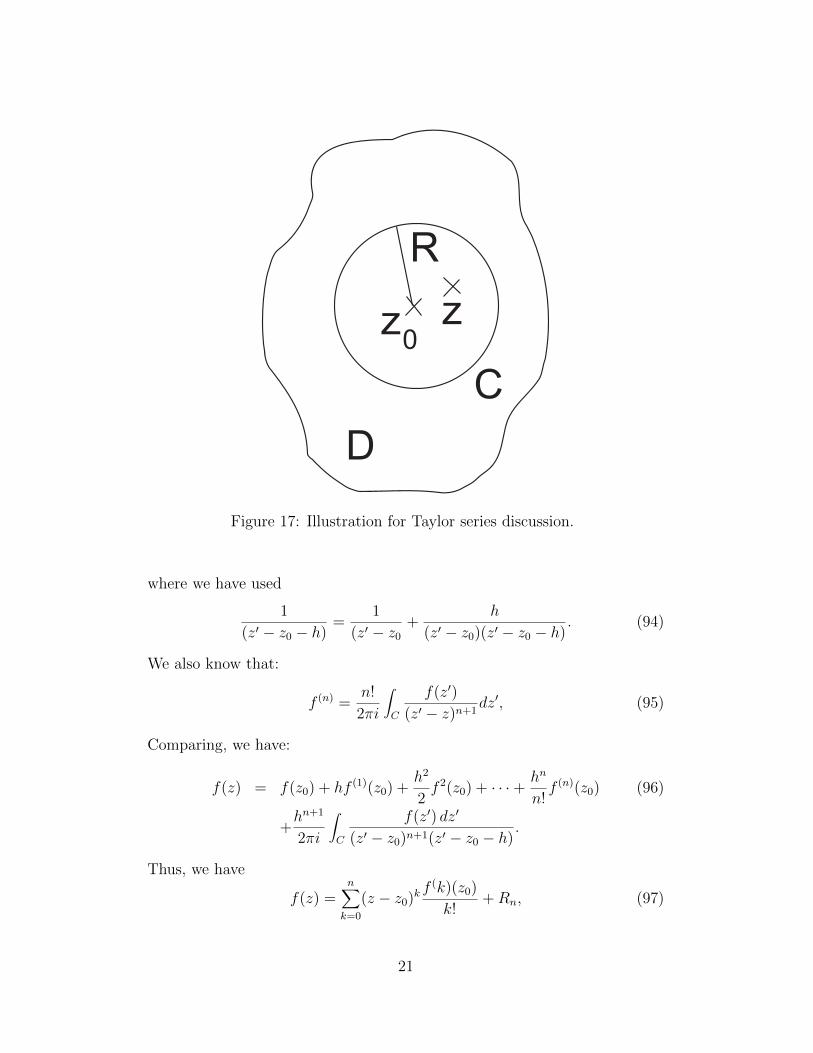
C

D

R

zz0

Figure 17: Illustration for Taylor series discussion.

where we have used

1

(z′ − z0 − h)=

1

(z′ − z0

+h

(z′ − z0)(z′ − z0 − h). (94)

We also know that:

f (n) =n!

2πi

∫C

f(z′)

(z′ − z)n+1dz′, (95)

Comparing, we have:

f(z) = f(z0) + hf (1)(z0) +h2

2f 2(z0) + · · ·+ hn

n!f (n)(z0) (96)

+hn+1

2πi

∫C

f(z′) dz′

(z′ − z0)n+1(z′ − z0 − h).

Thus, we have

f(z) =n∑k=0

(z − z0)kf (k)(z0)

k!+Rn, (97)

21

where

Rn =(z − z0)n+1

2πi

∫C

f(z′) dz′

(z′ − z0)n+1(z′ − z). (98)

We see that term by term this is the same form as the Taylor series expansionfor a real function of a real variable.

Let us investigate the remainder term, Rn. In particular, how big is it?We first notice that f(z′) and 1/|z′ − z| are continuous, hence bounded, onC: ∣∣∣∣∣ f(z′)

z′ − z

∣∣∣∣∣ ≤M, z′ ∈ C, z inside C. (99)

Let R be the radius of C. Then:

|Rn| =1

2π

∣∣∣∣∣(z − z0)n+1∫C

f(z′) dz′

(z′ − z0)n+1(z′ − z)

∣∣∣∣∣≤ M

2π|z − z0|n+1 1

Rn+12πR

≤ MR∣∣∣∣z − z0

R

∣∣∣∣n+1

. (100)

Since∣∣∣ z−z0R

∣∣∣ < 1, we can approximate f(z) to any desired accuracy with ourfinite Taylor series expansion.

10 Bolzano-Weierstrass Theorem

We wish to consider infinite series next, which means we must concern our-selves with issues of convergence. Let us begin with sequences. Given anysequence of complex numbers, z1, z2, . . . ≡ {zn}, we say that the sequence{zn} tends to the limit L as n→∞:

limn→∞

zn = L, (101)

if, for every ε > 0, there exists N such that |zN+k − L| < ε for all positiveintegers k. If {zn} is such that for any real number G, we can find N so that|zN+k| > G for all positive intergers k, then we say that |zn| tends to ∞ asn→∞.

Finally, if a sequence does not tend to a unique limit, and does not tendto plus or minus infinity, then the sequence is said to oscillate.

Definition: A limit point of a set S is a point such that there are anunlimited number of elements of S which are arbitrarily close to thelimit point.

22

For example, 1 is a limit point for the sequence 1 + 1/n (even though 1 isnot an element of the sequence). For another example, 1 is a limit point forthe sequence 1, 2, 1, 2, 1, 2, 1, 2, . . .

Theorem: (Bolzano-Weierstrass) If {xn} is an infinite sequence of real num-bers, and there exists a, b such that a ≤ xn ≤ b for all n (where a andb are independent of n), then {xn} has at least one limit point.

Proof: Let G be a real number such that G > |a|, G > |b|. Then, G > |xn|for all n. Consider the interval I0 = (−G,G). Cut it in half (say, to(−G, 0) and [0, G)): At least one subinterval must contain an infinitenumber of members of the sequence {xn}. Call the rightmost suchinterval I1. Now cut I1 in half. Again, at least one subinterval mustcontain an infinite number of members of the sequence {xn}. Call therightmost such interval I2. We may continue this interval subdivisionindefinitely, making our interval as small as we please. In the nested setof intervals I1, I2, I3, . . . there exists a point L which belongs to all theintervals of the nest. Choose k sufficiently large such that the lengthof Ik is less than any given ε > 0. Then if {x′n}k is the infinite set ofmembers of {xn} which lies in Ik, we have that |x′n − L| < ε for allmembers of {x′n}k. Hence L is a limit point of the sequence.

11 Cauchy’s Condition for the Existence of a

Limit, or, Cauchy’s Principle of Conver-

gence

Theorem: A sequence of complex numbers z1, z2, . . . has a limiting value ifand only if, given any ε > 0 there is an N such that |zN+k − zN | < εfor all positive integers k.

This convergence condition is referred to as Cauchy’s condition. Note thedistinction between this theorem and the definition of the limiting value. Toapply this test, one does not need to know, a priori, what the limit is.

Proof: Necessity: We suppose a limit, L, exists. Then, given any ε > 0,there exists an N such that |zN − L| < ε/2, and |zN+k − L| < ε/2 forall positive integers k. By the triangle inequality:

|zN+k − zN | ≤ |zN+k − L|+ |zN − L| < ε. (102)

23

Sufficiency: We suppose that given an ε > 0 there exists an N suchthat |zN+k − zN | < ε for all positive integers k. But the hypoteneuseof a triangle is longer than either other leg, and hence:

ε > |zN+k − zN | ≥ |xN+k − xN | (103)

≥ |yN+k − yN |. (104)

Thus, we may consider a real sequence {xn} which satisfies the Cauchycondition. Consider ε = 1, and pick an N = M such that:

|xM+k − xM | < 1 ∀k = 1, 2, 3, . . . (105)

Let a1, b1 be the least and greatest values, respectively, of the finitesequence x1, x2, . . . , xM . Let a = a1−1 and b = b1+1. Then a < xn < bfor all n. By the Bolzano-Weierstrass theorem, {xn} has at least onelimit point, G.

Now we must demonstrate that there is only one limit point: Supposethere are at least two, G and H. Then, given ε > 0, there exists ann such that |xn+p − xn| < ε, by hypothesis, and there exists positiveintegers q and r such that |G− xn+q| < ε and |H − xn+r| < ε, since Gand H are limit points. Thus,

|G−H| = |G− xn+q + xn+q − xn + xn − xn+r + xn+r −H|≤ |G− xn+q|+ |xn+q − xn|+ |xn+r − xn|+ |H − xn+r|< 4ε. (106)

Hence G=H, and there is only one limit point. Thus, given δ > 0,there are at most a finite number of terms of the sequence outside theinterval (G− δ,G+ δ), so G is the limit of {xn}.Similarly, the imaginary part sequence has a limit, hence {zn} hasa limit [noting that if limn→∞ zn = L, and limn→∞ z

′n = L′, then

limn→∞(zn + z′n) = L+ L′].

12 Infinite Series

Given a sequence {un}, we can construct a sequence:

S0 = u0 (107)

S1 = u0 + u1 (108)...

Sn =n∑k=0

uk. (109)

24

These are the “partial sums” of the infinite series:

S =∞∑k=0

uk. (110)

The infinite series is said to converge if, given ε > 0 there exists S andn0 such that:

|S − Sn| < ε, ∀n > n0. (111)

If the series∑∞n=0 un converges: It is said to be absolutely convergent if∑∞

n=0 |un| converges; otherwise it is conditionally convergent. Note that anabsolutely convergent series may be rearranged at will, with identical results,but this doesn’t hold for a conditionally convergent series.

We give some tests for convergence, leaving the proofs to the reader:

1. Cauchy Integral test for convergence: If f(x) is a positive, real,decreasing function of x for real x ≥ 1, then the series S =

∑∞n=1 f(n)

converges or diverges, depending on whether the integral

limn→∞

∫ n

1f(x)dx (112)

converges or diverges.

2. Comparison test for absolute convergence: S =∑∞n=0 un is absolutely

convergent if|un| < c|vn|, ∀n > N, (113)

c is independent of n, and∑∞n=0 vn is known to be absolutely convergent.

3. d’Alembert’s ratio test for absolute convergence:∑∞n=0 un converges

absolutely if

limn→∞

∣∣∣∣un+1

un

∣∣∣∣ < 1, (114)

where lim is the “limit superior”, or least upper bound of all convergentsubsequences of {un}. The sum diverges if

limn→∞

∣∣∣∣un+1

un

∣∣∣∣ > 1. (115)

4. Raabe’s test for absolute convergence: If

limn→∞

∣∣∣∣un+1

un

∣∣∣∣ = 1, (116)

and

limn→∞n(∣∣∣∣un+1

un

∣∣∣∣− 1)< −1, (117)

then∑∞n=0 un converges absolutely.

25

5. Cauchy’s test for absolute convergence: If

limn→∞ |un|1/n < 1, (118)

then∑∞n=0 un converges absolutely.

13 Series of Functions

If the terms of an infinite series are functions of complex variable z, then theseries may converge or not, depending on the value of z. We are interestedin the region of convergence of such a series. We are also interested incontinuity, integrability, and differentiability of such a series (especially ofanalytic functions, including power series).

If S(z) =∑∞n=0 un(z) and SN(z) =

∑Nn=0 un(z), then S(z) is said to be

uniformly convergent over the set of points {z|z ∈ R} = R if, given anyε > 0, there exists an N such that:

|S(z)− SN+k(z)| < ε, ∀k = 0, 1, 2, . . . , and ∀z ∈ R. (119)

Note that the condition of uniform convergence is in a sense stronger thansimple convergence – S(z) may converge for all z ∈ R, without being uni-formly convergent. As an example, consider f(z) = 1/(1 − z), for R = {z :|z| < 1}.

A necessary and sufficient condition for uniform convergence is “Cauchy’sprinciple for uniform convergence: Given S(z) =

∑∞n=0 un(z) which converges

for all z ∈ R, where R is a closed region, and any ε > 0, then S(z) convergesuniformly in R if there exists an N such that

|SN(z)− SN+k(z)| < ε, ∀k = 0, 1, 2, . . . , and ∀z ∈ R. (120)

It is left to the reader to prove this, using techniques similar to methodsalready encountered.

Another, sufficient, test for uniform convergence is the “Weierstrass Mtest”: If |un(z)| ≤ Mn, where Mn is a positive real number, independentof z ∈ R, and if

∑∞n=0Mn converges, then S(z) is uniformly convergent on

z ∈ R.Let us consider the following example: Suppose we have the real series

S(x) = x2 +x2

1 + x2+

x2

(1 + x2)2+ · · · (121)

=∞∑n=0

x2

(1 + x2)n. (122)

26

We see that S(x) converges absolutely for all real x, since:

SN(x) =N∑n=0

x2

(1 + x2)n(123)

=

{0 if x = 0,1 + x2 − 1

(1+x2)Nif x 6= 0. (124)

Thus, S(x) converges absolutely for all possible real x values.But does this series converge uniformly? We suspect trouble because of

the peculiar behavior at x = 0:

S(x) ={

0 at x = 0,1 + x2 for x 6= 0.

(125)

That is, S(x) is discontinuous at x = 0. For uniform convergence, we musthave the case that, given any ε > 0 there exists an N , independent of x, suchthat

|SN(x)− SN+k(x)| < ε, ∀k = 0, 1, 2, . . . , and ∀x. (126)

Assume x > 0. Then:

|SN(x)− SN+k(x)| = 1

(1 + x2)N+k. (127)

Let’s choose ε = 1/2. Notice that for any fixed N , and any chosen k, we canalways pick x > 0 small enough so that

1

(1 + x2)N+k>

1

2= ε. (128)

Hence the convergence is not uniform near x = 0.The following theorem addresses the question of continuity:

Theorem: If S(z) =∑∞n=0 un(z) is a uniformly convergent series of continu-

ous functions un(z) for all z ∈ R, where R is a closed region, then S(z)is a continuous function of z, for all z ∈ R.

Proof: Write S(z) = Sn(z)+Rn(z), where Rn(z) =∑∞k=1 un+k(z). Sn(z) is a

finite sum of continuous functions and hence is continuous throughoutR. By uniform convergence, given any ε > 0, we can find N such thatRN(z) < 1

3ε, for all z ∈ R. Furthermore, since SN(z) is continuous for

all z ∈ R, there exists a ρ > 0 such that |SN(z + δ) − SN(z)| < 13ε

whenever |δ| < ρ and z + δ ∈ R. Therefore:

|S(z + δ)− S(z)| = |SN(z + δ)− SN(z) +RN(z + δ)−RN(z)|≤ |SN(z + δ)− SN(z)|+ |RN(z + δ)|+ |RN(z)|< ε. (129)

Hence, S(z) is continuous for all z ∈ R.

27

We may also be concerned with the question of multiplication of series. Iftwo series are absolutely convergent, then the series formed of product termsis absolutely convergent independent of order, and the product series is equalto the product of the individual series.

Next, let us consider the integration of a series:

Theorem: Let S(z) =∑∞n=0 be a uniformly convergent series of continuous

functions in a domain D. Then, if C ⊂ D, where C is a finite path inD, we have: ∫

CS(z)dz =

∞∑n=0

∫Cun(z)dz. (130)

The order of integration and summation may be interchanged for aseries of continuous functions in its domain of uniform convergence.

Proof: Write S(z) =∑nk=0 uk(z) + Rn(z), where Rn(z) =

∑∞k=1 un+k(z).

Then ∫CS(z)dz =

n∑k=0

∫Cuk(z)dz +

∫CRn(z)dz. (131)

Since S(z) is uniformly convergent, for any given ε > 0, there existsan N such that Rn(z) < ε for all n ≥ N and all z ∈ D. Now, ifLC =

∫C |dz| <∞ is the “path length”, then∣∣∣∣∫

CRn(z)dz

∣∣∣∣ < εLC , ∀n ≥ N. (132)

Hence, ∣∣∣∣∣∫CS(z)dz −

n∑k=0

∫Cuk(z)dz

∣∣∣∣∣ < εLC , ∀n ≥ N, (133)

which can be made arbitrarily small.

Next, we investigate the differentiation of a series.

Theorem: If S(z) =∑∞n=0 un(z) is a series of functions which are analytic

on and inside a contour C, and if S(z) converges uniformly on C, thenS(z) is analytic everywhere inside C, with derivative:

dS

dz(z) =

∞∑n=0

dundz

(z). (134)

That is, The order of differentiation and summation may be reversed.

28

Proof: Let z0 be a point inside C.

1

2πi

∫C

S(z)dz

z − z0

=1

2πi

∫C

[ ∞∑n=0

un(z)

]dz

z − z0

=1

2πi

[∫C

n∑k=0

uk(z)

z − z0

dz +∫C

Rn(z)

z − z0

dz

]

=n∑k=0

uk(z0) +1

2πi

∫C

Rn(z)

z − z0

dz. (135)

The series converges uniformly on C, so given any ε > 0 there existsan N such that |Rk(z)| < ε for all k ≥ n and for all z ∈ C. Thus,∣∣∣∣∣

∫C

Rn(z)

z − z0

dz

∣∣∣∣∣ < ε

∣∣∣∣∣∫C

dz

z − z0

∣∣∣∣∣ < 2πε. (136)

Therefore, the series converges, and we have:

1

2πi

∫C

S(z)

z − z0

dz =∞∑n=0

un(z0) ≡ S(z0), (137)

where we take the latter as the definition of S(z0) interior to C.

Thus, S(z) =∑∞n=0 un(z) is defined on and inside C. To prove analyt-

icity inside C, we show that the derivative exists:

S ′(z0) = limh→0

S(z0 + h)− S(z0)

h

= limh→0

1

2πi

1

h

∫C

[S(z)

z − z0 − h− S(z)

z − z0

]dz

= limh→0

1

2πi

∫C

S(z)

(z − z0 − h)(z − z0)dz

=1

2πi

[n∑k=0

∫C

uk(z)

(z − z0)2dz +

∫C

Rn(z)

(z − z0)2dz

]. (138)

The first term is the form of the derivative of an analytic function wesaw earlier. The second term can be made arbitrarily small by takingn large enough, by the uniform convergence of S on C. Hence,

S ′(z) =∞∑n=0

dundz

(z). (139)

Let us now turn to the special case of power series, of which the Taylorseries is an important example.

29

Theorem: If S(z) =∑∞n=0 anz

n converges for z = z1, then it is absolutelyconvergent for all |z| < |z1|.

Proof: Since the series converges for z = z1, anzn1 must be bounded: |anzn1 | <

M for all n. Pick any z such that |z| < |z1|. Let r = |z|/|z1| < 1. Then

|anzn| = |anzn1 |∣∣∣∣ zz1

∣∣∣∣n < Mrn, (140)

and ∞∑n=0

|anzn| <∞∑n=0

Mrn = M∞∑n=0

rn. (141)

Since r < 1, this is convergent, hence S(z) is absolutely convergent forall |z| < |z1|.

A similar argument can be used to show that, if S(z) =∑∞n=0 anz

n di-verges for z = z1, then it diverges for all |z| > |z1|. Thus, the region ofconvergence of a power series is a circle: Inside the circle there is absoluteconvergence, and outside there is divergence. On the circle, we cannot sayin general. For example,

S(z) =∞∑n=1

zn

n

diverges for |z| > 1absolutely converges for |z| < 1converges for z = −1diverges for z = +1.

(142)

We state and leave it for the reader to prove the following:

Theorem: A power series is uniformly convergent in any closed region insidethe circle of convergence.

We have the following uniqueness theorem for power series:

Theorem: If S(z) =∑∞n=0 an(z − z0)n converges for all points inside the

circle |z − z0| = r0, then the series is the Taylor series for S(z) (aboutz0).

Proof: The proof consists in differentiating k times, and showing that an =S(n)(z0)/n!.

30

×

C

Cz

z

1

2

0

Figure 18: Illustration for Laurent series discussion.

14 Laurent Series

We now introduce a generalizaton of the Taylor series, the Laurent series.Consider a function f(z) which is analytic in a region containing two con-centric circles (but not necessarily in the interior of the smaller circle).

“Contour” C2−C1 (Fig. 18 represents a closed path in a “simply-connected”domain, so we can use the Cauchy Integral Formula (for z in the annulus):

f(z) =1

2πi

∫C2

f(z′)

z′ − zdz′ − 1

2πi

∫C1

f(z′)

z′ − zdz′. (143)

Now,1

z′ − z=

1

z′ − z0

· 1

1− (z − z0)/(z′ − z0). (144)

For z′ on C2, z in the annulus, and with z0 the center of the circles, |(z −z0)/(z′ − z0)| < 1. We may thus write, for z′ on C2:

1

z′ − z=∞∑n=0

(z − z0)n

(z′ − z0)n+1. (145)

Similarly, for z′ on C1:

− 1

z′ − z=∞∑n=0

(z′ − z0)n

(z − z0)n+1. (146)

31

Putting this back into 143:

f(z) =∞∑n=0

[(z − z0)n

2πi

∫C2

f(z′)

(z′ − z0)n+1dz′ − 1

2πi

1

(z − z0)n+1

∫C1

(z′ − z0)nf(z′) dz′].

(147)Thus, we can write:

f(z) =∞∑n=0

an(z − z0)n +∞∑n=1

bn1

(z − z0)n, (148)

where:

an =1

2πi

∫C2

f(z′)

(z′ − z0)n+1dz′, n = 0, 1, 2, . . . (149)

bn =1

2πi

∫C1

f(z′)

(z′ − z0)−n+1dz′, n = 1, 2, . . . (150)

Or, we may combine the series:

f(z) =∞∑

n=−∞An(z − z0)n, (151)

where,

An =1

2πi

∫C

f(z′)

(z′ − z0)n+1dz′, (152)

where C is any contour which makes one counter-clockwise passage aroundz0, and lies in the region bounded by C1 and C2. This is called the Laurentseries.

If we express f(z) = φ(z) + ψ(z), where

φ(z) =∞∑n=0

An(z − z0)n, (153)

ψ(z) =∞∑n=1

A−n(z − z0)−n, (154)

then ψ(z) is called the principal part of f(z). Note that φ(z) convergesuniformly in any closed region interior to the outer edge of the annulus.Hence, f(z) = φ(z) + ψ(z) converges uniformly in any closed region withinthe annulus.

If z = z0 is a singularity of f(z), and there exists a neighborhood of z0

which contains no other singularity, then z0 is called an isolated singularityof f(z). For example, z = 1 is an isolated singularity of f(z) = 1/(z − 1). If

32

all the coefficients of the principal part vanish, then an isolated singularity z0

is called a removable singularity. For example, the origin is a removablesingularity of f(z) = sin z/z. The singularity in this case may be “removed”by defining

f(0) ≡ limz→0

sin z

z= 1. (155)

If the principal part terminates after a finite number of terms, say

A−m 6= 0, (156)

A−(m+k) = 0, ∀k = 1, 2, 3, . . . , (157)

then f(z) is said to have a pole of order mmm at z0. For example, f(z) =1/(z − z0)2 has a pole of order 2 at z0.

If the principal part has an infinite number of non-vanishing coeeficients,then z0 is called an essential singularity of f(z). An essential singularityneed not be isolated. For example, z = 0 is an essential singularity of f(z) =1/ sin(1/z). It is also the limit point of a sequence of poles, and hence isnot an isolated singularity. On the other hand, z = 0 is an isolated essentialsingularity of f(z) = e1/z.

If the Laurent series is not known, the order of a pole may be determinedby examining limits. Consider the limits:

limz→z0

(z − z0)nf(z), n = 1, 2, 3, . . . (158)

The lowest n for which the limit exists is the order of the pole at z0.

15 Residues

Consider the integral:

In =∫C

(z − z0)n dz, (159)

where C is a closed contour surrounding z = z0 and n is an integer. Since(z− z0)n is analytic, except possibly at z0, we may deform the contour into acircle centered at z0 without affecting In. Then we may write z − z0 = Reiθ,and hence

In = iRn+1∫ 2π

0ei(n+1)θ dθ. (160)

={

0 n 6= −12πi n = −1

. (161)

33

Now suppose we have a function, f(z), which is analytic in a region exceptat the point z0 in the region. Then we can make the Laurent expansion aboutz0:

f(z) =∞∑

n=−∞An(z − z0)n. (162)

Take a contour C around z0:

1

2πi

∫Cf(z) dz =

1

2πi

∫C

∞∑n=−∞

An(z − z0)n dz (163)

= A−1. (164)

Thus the coefficient of 1/(z − z0) in the Laurent series is given by A−1 =1

2πi

∫C f(z)dz. This coefficient is called the residue of f(z) at z0. Notice

that the residue is zero if f(z) is analytic at z0, or if the coefficient A−1 iszero (even if z0 is a pole or isolated essential singularity).

We now come to the important and useful residue theorem. Considercontour C in a region where f(z) is analytic except at isolated singularities(poles or essential singularities).

×

×

×

C

CC

C

ab

c

ab

c

Figure 19: Contours to illustrate residue theorem. Singularities are at a, b,and c.

We want to determine∫C f(z) dz. We can write this in terms of the sum

of the integrals around each singularity:∫Cf(z) dz =

∫Caf(z) dz +

∫Cb

f(z) dz + · · ·

34

= 2πi(a−1 + b−1 + c−1 + · · ·)= 2πi

∑singularities

R, (165)

where a−1, b−1, c−1, . . . are the residues at a, b, c, . . ., respectively, and∑R is

the sum of the residues of f(z) interior to the countour C.The computation of the residues is thus often an important part of eval-

uating integrals. At a simple pole, the Laurent series is

f(z) =A−1

z − z0

+∞∑n=0

An(z − z0)n, (166)

and henceA−1 = lim

z→z0[(z − z0)f(z)] . (167)

For a pole of order m,

f(z) =A−m

(z − z0)m+

A−m+1

(z − z0)m−1+ · · ·+ A−1

z − z0

+∞∑n=0

An(z − z0)n. (168)

If we multiply both sides by (z − z0)m, we have:

(z−z0)mf(z) = A−m+A−m+1(z−z0)+· · ·+A−1(z−z0)m−1+∞∑n=0

An(z−z0)n+m.

(169)Now differentiate m− 1 times and evaluate at z = z0:

dm−1 [(z − z0)mf(z)]

dzm−1

∣∣∣z=z0

= (m− 1)!A−1, (170)

and hence,

A−1 =1

(m− 1)!

dm−1 [(z − z0)mf(z)]

dzm−1

∣∣∣z=z0

. (171)

But sometimes it is easier to just carry out the expansion sufficiently to findA−1 directly.

16 Cauchy Principal Value Integral

Suppose f(z) has a simple pole at z = z0 = x0 + i0 on the real axis. We maydefine an integral along the real axis through this pole according to:

P∫ β

αf(z)dz ≡ lim

ε→0

[∫ x0−ε

αf(x)dx+

∫ β

x0+εf(x)dx

], (172)

where α < x0 < β. This is known as the Cauchy Principal Value Inte-gral.

35