15/10/2014

1

Respon Biner

15/10/2014

2

Regresi Logistik

4.1 INTERPRETING THE LOGISTIC REGRESSION MODEL4.2 INFERENCE FOR LOGISTIC REGRESSION

Model regresi logistik menggunakan peubah

j l b ik k t ik t k ti t kpenjelas, baik kategorik atau kontinu, untuk

memprediksi peluang dari hasil yang spesifik.

Dengan kata lain regresi logistik dirancang untukDengan kata lain, regresi logistik dirancang untuk

menggambarkan peluang yang terkait dengan nilai‐

nilai peubah respon.

15/10/2014

3

• Kurva regresi logistik dan regresi linier

15/10/2014

4

• β>0 maka kurva akan naik

β<0 k k k t• β<0 maka kurva akan turun

• Jika β= 0 maka nilai π (x) tetap pada berapapun nilai x          kurva akan menjadi garis horisontal

• X  Peubah penjelas kuantitatif• Y  Peubah respon biner

4.1 INTERPRETING THE LOGISTIC REGRESSION MODEL

• π(x)  peluang sukses peubah X• Model Logit (log odds)

15/10/2014

5

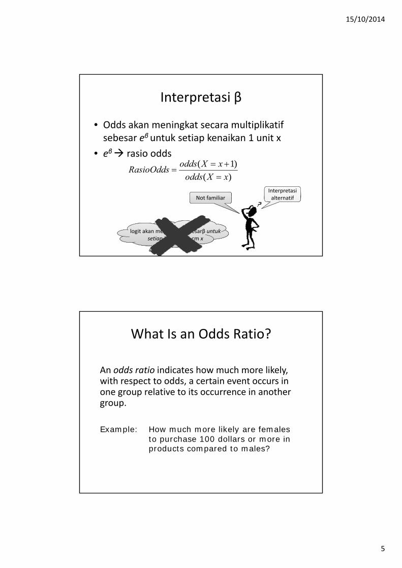
Interpretasi β

• Odds akan meningkat secara multiplikatif b β t k ti k ik 1 itsebesar eβuntuk setiap kenaikan 1 unit x

• eβ rasio odds

)()1(

xXoddsxXoddsRasioOdds=+=

=

Interpretasil ff ili

logit akan meningkat sebesarβ untuk setiap kenaikan 1 cm x

alternatifNot familiar

What Is an Odds Ratio?

An odds ratio indicates how much more likelyAn odds ratio indicates how much more likely, with respect to odds, a certain event occurs in one group relative to its occurrence in another group.

Example: How much more likely are females p yto purchase 100 dollars or more in products compared to males?

15/10/2014

6

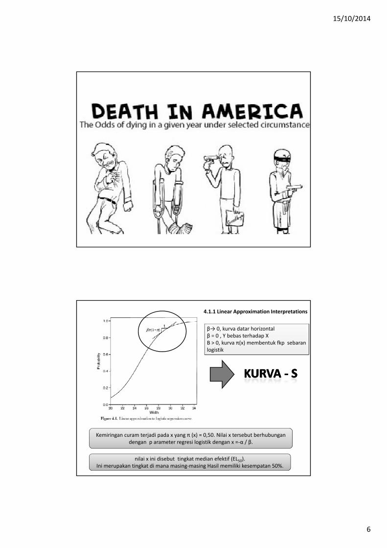
4.1.1 Linear Approximation Interpretations

β→ 0, kurva datar horizontalβ = 0 , Y bebas terhadap XΒ > 0, kurva π(x) membentuk fkp  sebaran logistik

Kemiringan curam terjadi pada x yang π (x) = 0,50. Nilai x tersebut berhubungan dengan  p arameter regresi logistik dengan x =‐α / β. 

nilai x ini disebut  tingkat median efektif (EL50). Ini merupakan tingkat di mana masing‐masing Hasil memiliki kesempatan 50%. 

15/10/2014

7

4.1.2 Horseshoe Crabs: Viewing and Smoothing a Binary Outcome

The study investigated factors that affect whether the female crab had any othermales, called satellites, residing nearby her. The response outcome for each femalecrab is her number of satellites. An explanatory variable thought possibly to affect

ilustrasi

crab is her number of satellites. An explanatory variable thought possibly to affectthis was the female crab’s shell width, which is a summary of her size. In the sample,this shell width had a mean of 26.3 cm and a standard deviation of 2.1 cm.

Y indicate whether a female crab has any satellites (other males who could mate with her). That is, Y = 1 if a female crab has at least one satellite, and Y = 0 if she has no satellite.We first use the female crab’s width (in cm) as the sole predictor.

• Suatu penelitian mengenai faktor‐faktor yang mempengaruhi banyaknya satellite yang

ilustrasi

mempengaruhi banyaknya satellite yang dipunyai kepiting betina (Y)

• Y= 1 jika kepiting betina memiliki paling tidak 1 satellite Y=0  jika tidak memiliki satellite. 

• X= lebar cangkang kepiting betina (dalam cm)

15/10/2014

8

• Data yang belum dikelompokkan 

Syntax SASData crab; input width sat;d lidatalines; 28.3 126.0 125.6 0...24.5 04.5 0; proc logistic data=crab descending; 

model sat=width/expb; run;

15/10/2014

9

Output

At the minimum width in this sample of 21.0 cm, the estimated probability isexp(−12.351 + 0.497(21.0))/[1 + exp(−12.351 + 0.497(21.0))] = 0.129

At the maximum width of 33.5 cm, the estimated probability equalsexp(−12.351 + 0.497(33.5))/[1 + exp(−12.351 + 0.497(33.5))] = 0.987

• lebar minimum x= 21 cm, 

= 0.129

• lebar maksimum x= 33.5 cm

= 0.987

15/10/2014

10

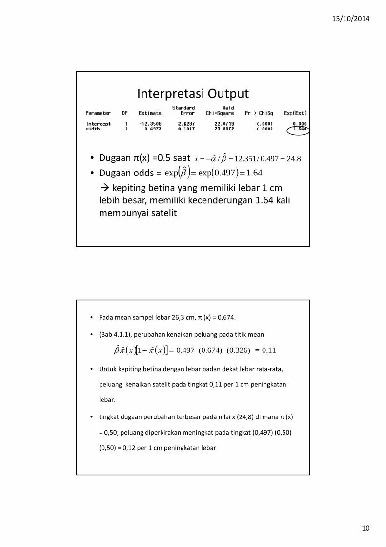
Interpretasi Output

• Dugaan π(x) =0.5 saat• Dugaan odds =

kepiting betina yang memiliki lebar 1 cm

8.24497.0/351.12ˆ/ˆ ==−= βαx

( ) ( ) 64.1497.0expˆexp ==β

kepiting betina yang memiliki lebar 1 cm lebih besar, memiliki kecenderungan 1.64 kali mempunyai satelit

• Pada mean sampel lebar 26,3 cm, π (x) = 0,674. 

• (Bab 4.1.1), perubahan kenaikan peluang pada titik mean

( ) ( )[ ] 0.11 = (0.326) (0.674) 0.497ˆ1ˆˆ =− xx ππβ

• Untuk kepiting betina dengan lebar badan dekat lebar rata‐rata, 

peluang  kenaikan satelit pada tingkat 0,11 per 1 cm peningkatan 

lebar.

• tingkat dugaan perubahan terbesar pada nilai x (24 8) di mana π (x)• tingkat dugaan perubahan terbesar pada nilai x (24,8) di mana π (x) 

= 0,50; peluang diperkirakan meningkat pada tingkat (0,497) (0,50) 

(0,50) = 0,12 per 1 cm peningkatan lebar

15/10/2014

11

Berbeda dengan model peluang linier, model regresi logistik

memungkinkan laju perubahanmemungkinkan laju perubahan bervariasi sebagaimana perubahan x

Regression Fit

• Model paling sederhana untuk interpretasi d l h d l l ( ) βadalah model peluang π(x) = α + βx.

• Menggunakan pendekatan OLS (software GLM dengan asumsi respon normal dengan fungsi penghubung identitas) menghasilkan model

15/10/2014

12

Proc GLMproc genmod data=crab;

model sat=width/ dist = norlink = identitylink = identitylrci;

run;

4.1.3 Horseshoe Crabs: Interpreting the Logistic Regression Fit

• π(x) adalah peluang kepiting betina memiliki satelit dengan lebar badan x cm

• Dugaan peluang (adanya) satelit akan meningkat 0.092 untuk setiap peningkatan 1 cm lebar badan kepiting

• Interpretasi  lebih sederhana, namun tidak sesuai untuk nilai ekstrimMi lk d h i i l b b d• Misalkan pada contoh ini lebar badan maksimal 33.5 cm. Dugaan peluangnya= −1.766 + 0.092(33.5) = 1.3.

15/10/2014

13

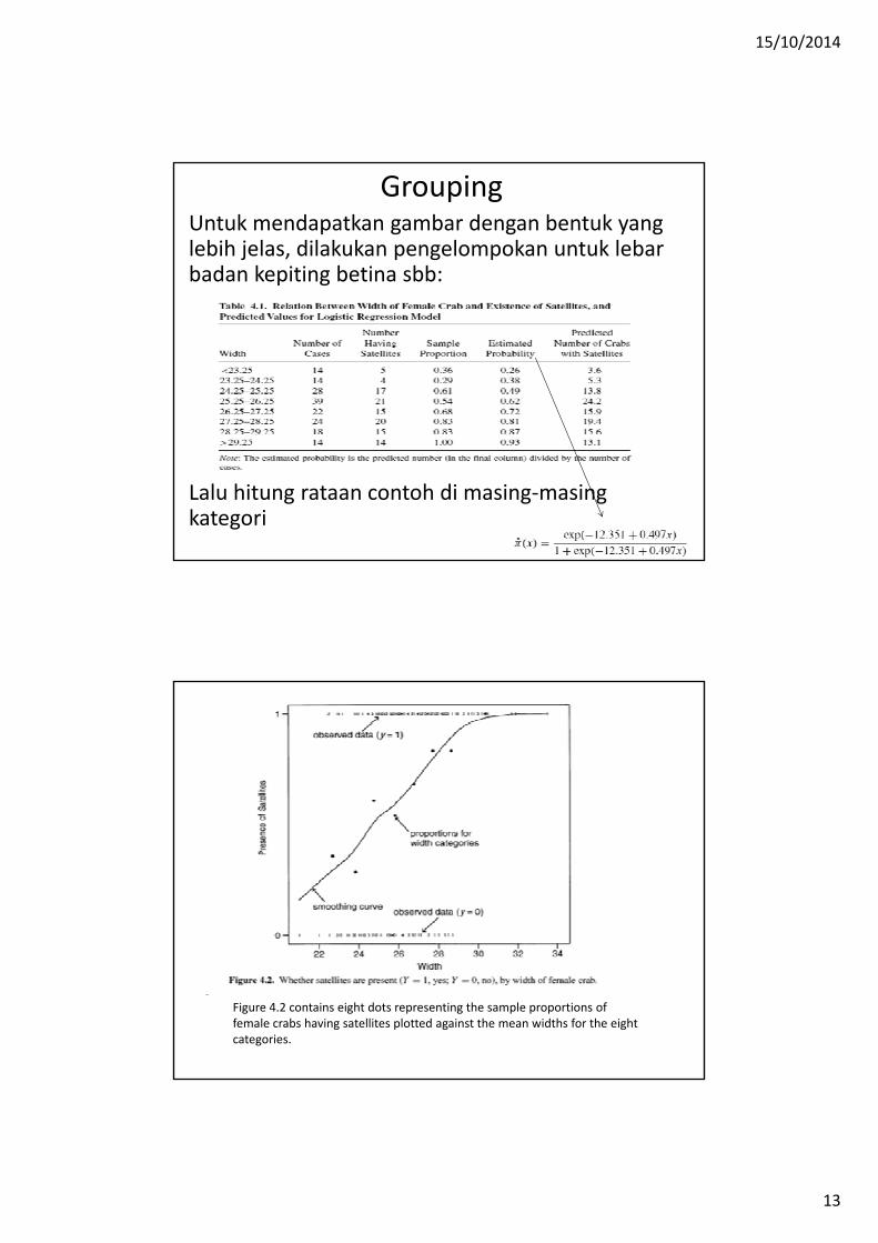
GroupingUntuk mendapatkan gambar dengan bentuk yang lebih jelas, dilakukan pengelompokan untuk lebar badan kepiting betina sbb:

Lalu hitung rataan contoh di masing‐masing kategori

Figure 4.2 contains eight dots representing the sample proportions of female crabs having satellites plotted against the mean widths for the eight categories.

15/10/2014

14

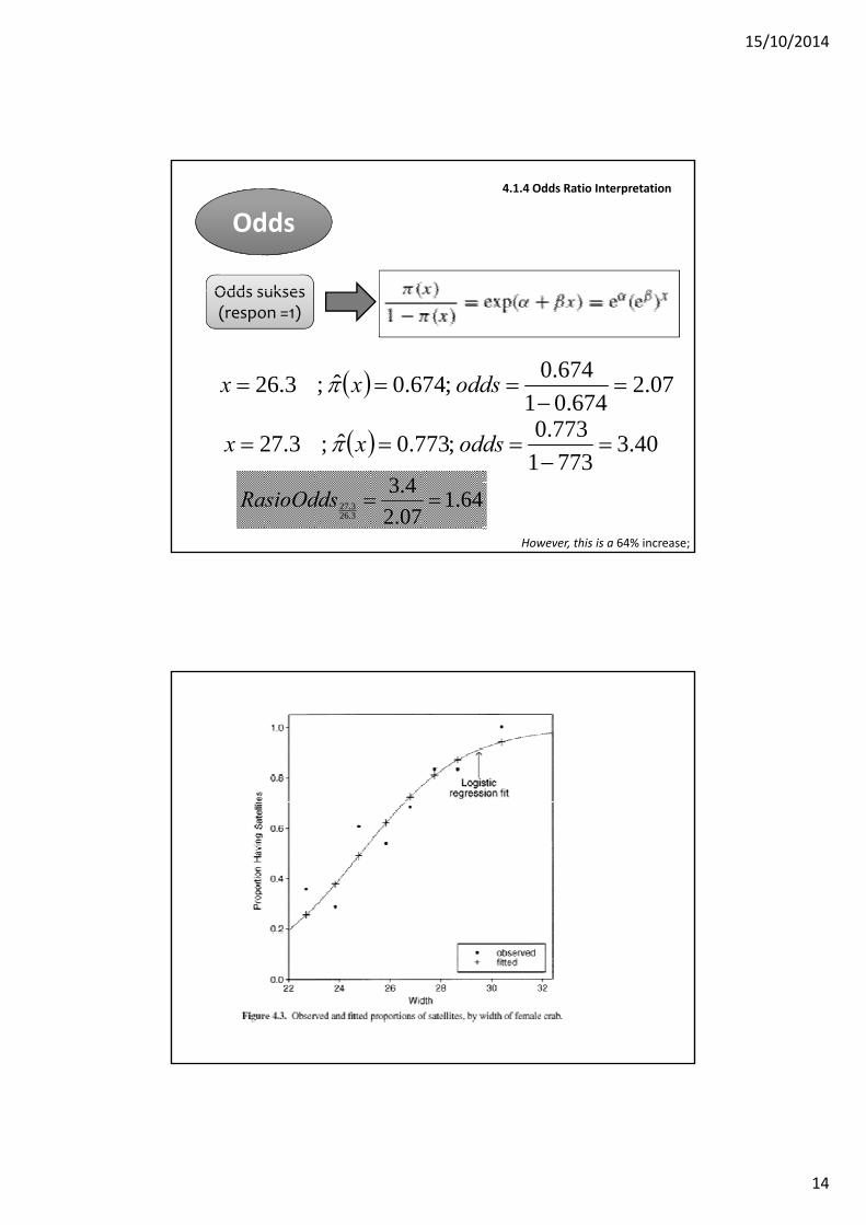
4.1.4 Odds Ratio Interpretation

Odds

Odds sukses Odds sukses (respon =1)

( ) 07.2674.01

674.0;674.0ˆ;3.26 =−

=== oddsxx π

7730

However, this is a 64% increase; 

( ) 40.37731773.0;773.0ˆ;3.27 =−

=== oddsxx π

64.107.24.3

3.263.27 ==RasioOdds

15/10/2014

15

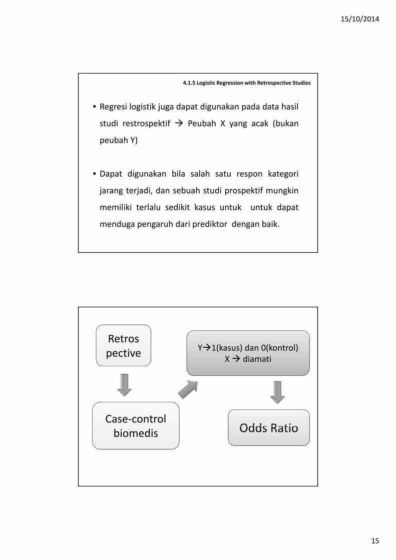
4.1.5 Logistic Regression with Retrospective Studies

• Regresi logistik juga dapat digunakan pada data hasil

studi restrospektif Peubah X yang acak (bukan

peubah Y)

• Dapat digunakan bila salah satu respon kategori

jarang terjadi, dan sebuah studi prospektif mungkinjarang terjadi, dan sebuah studi prospektif mungkin

memiliki terlalu sedikit kasus untuk untuk dapat

menduga pengaruh dari prediktor dengan baik.

Retros pective Y 1(kasus) dan 0(kontrol)

X  diamati

Case‐control Odds Ratiobiomedis Odds Ratio

15/10/2014

16

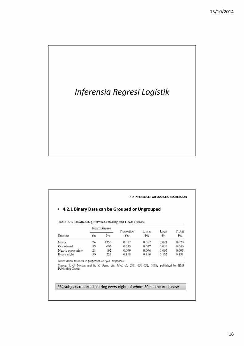
Inferensia Regresi Logistik

4.2 INFERENCE FOR LOGISTIC REGRESSION

• 4.2.1 Binary Data can be Grouped or Ungrouped

254 subjects reported snoring every night, of whom 30 had heart disease

15/10/2014

17

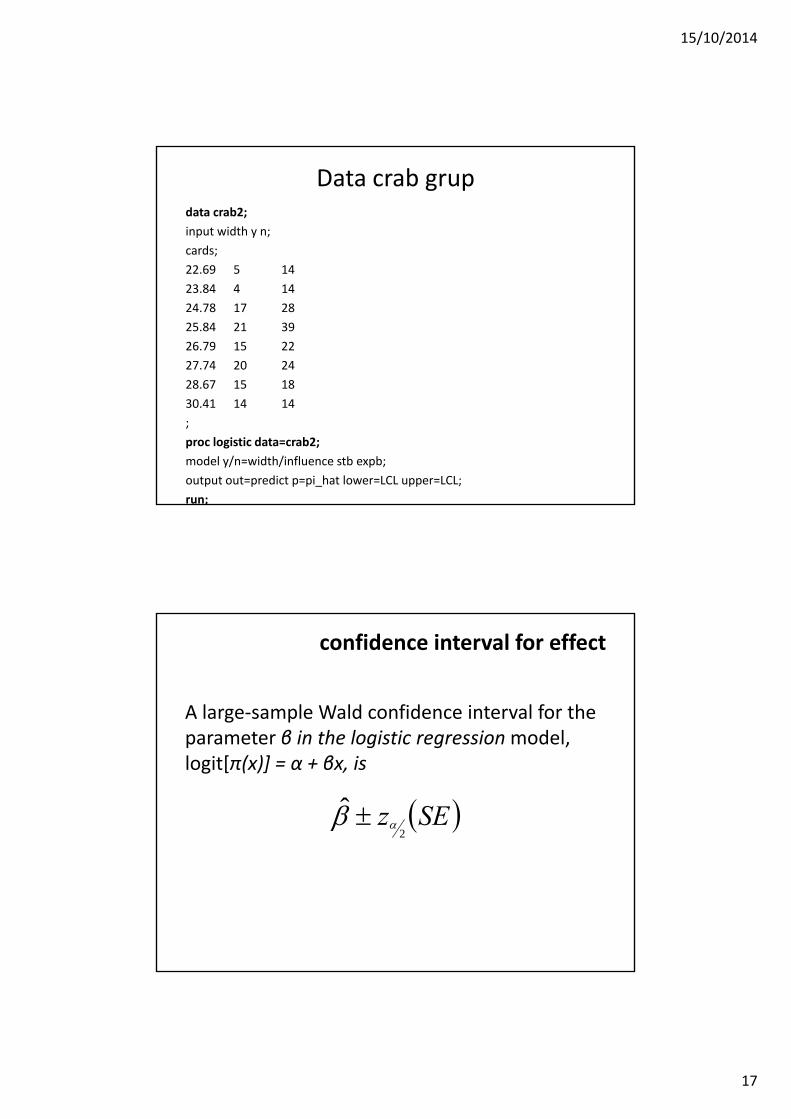
Data crab grupdata crab2;input width y n;cards;22 69 5 1422.69 5 1423.84 4 1424.78 17 2825.84 21 3926.79 15 2227.74 20 2428 67 15 1828.67 15 1830.41 14 14;proc logistic data=crab2;model y/n=width/influence stb expb;output out=predict p=pi_hat lower=LCL upper=LCL;run;

confidence interval for effect

A large‐sample Wald confidence interval for the t β i th l i ti i d lparameter β in the logistic regressionmodel, 

logit[π(x)] = α + βx, is

( )SEz2

ˆαβ ±

15/10/2014

18

Ilustrasi data kepiting

• Selang kepercayaan 95% untuk β adalah 0.497± 1.96(0.102) = [0.298, 0.697]

• Selang kepercayaan berdasarkan likelihood ratio = (0.308, 0.709).

• Interval likelihood ratio untuk pengaruh pada odds setiap kenaikan 1 cm lebar cangkang = (e308, e709)= (1.36, 2.03).

• Berarti setiap kenaikan 1 cm lebar cangkang, akan menaikkan odds satellite paling sedikit 1.36 kali dan paling banyak 2 kali

15/10/2014

19

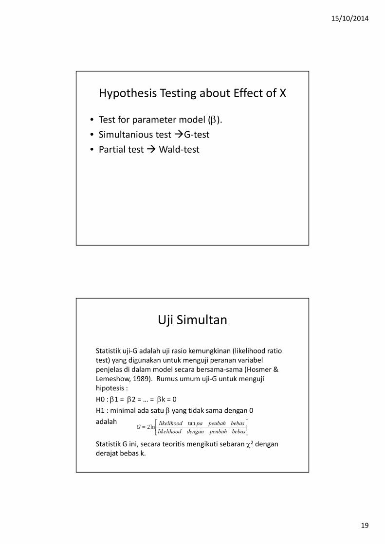
Hypothesis Testing about Effect of X

• Test for parameter model (β).  • Simultanious test  G‐test• Partial test  Wald‐test

Uji Simultan

Statistik uji‐G adalah uji rasio kemungkinan (likelihood ratio test) yang digunakan untuk menguji peranan variabelpenjelas di dalam model secara bersama‐sama (Hosmer & Lemeshow, 1989).  Rumus umum uji‐G untuk mengujihipotesis :H0 : β1 =  β2 = … =  βk = 0H1 : minimal ada satu β yang tidak sama dengan 0β y g gadalah

Statistik G ini, secara teoritis mengikuti sebaran χ2 dengan derajat bebas k.

⎥⎦

⎤⎢⎣

⎡=

bebaspeubahdenganlikelihoodbebaspeubahpalikelihoodG tanln2

15/10/2014

20

Partial TestSementara itu, uji Wald digunakan untuk menguji parameter βi secara parsial.  Hipotesis yang diuji adalah:H0 : βi = 0H1 : βi ≠ 0Formula statistik Wald adalah:

Secara teori, statistik Z ini mengikuti sebaran normal baku jika H0 benar.

)ˆ(

ˆ

i

i

SEZ

ββ

=

normal baku jika H0 benar.

Atau menggunakan statistik uji                          yang mengikuti sebaran         dengan db=1

Uji Hipotesi Data Kepiting• Hipotesis  H0 : β= 0 vs   H1 : β ≠ 0

• Statistik Uji :  Z= 0.497/0.102 = 4.9. (This shows strong evidence of a positive effect of width on the(This shows strong evidence of a positive effect of width on the presence of satellites (P <0.0001))

• The equivalent chi‐squared statistic, z2 = 23.9, has df = 1.

• Software reports that the maximized log likelihoods equal L0 = 

−112.88 under H0: β = 0 and L1 = −97.23 for the full model. The 

lik lih d ti t ti ti l 2(L0 L1) 31 3 ith df 1likelihood‐ratio statistic equals −2(L0 − L1) = 31.3, with df = 1.

• This also provides extremely strong evidence of a width effect (P < 

0.0001).

15/10/2014

21

Confidence Intervals for Probabilities

• We illustrate by estimating the probability of a satellite for female 

crabs of width x = 26.5, which is near the mean width. 

• The logistic regression fit yields

πˆ = exp(−12.351 + 0.497(26.5))/[1 + exp(−12.351 + 0.497(26.5))] = 

0.695

• From software, a 95% confidence interval for the true probability is 

(0.61, 0.77).

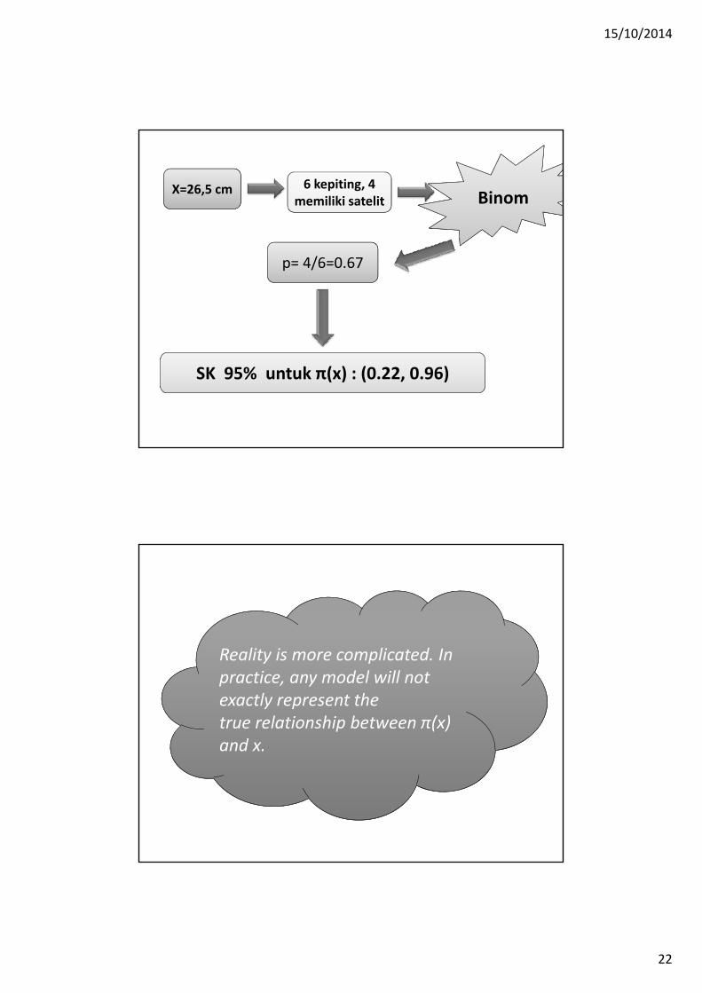
Kenapa menggunakan model untuk menduga 

peluang??

15/10/2014

22

X=26,5 cm 6 kepiting, 4 memiliki satelit Binom

p= 4/6=0.67

SK  95%  untuk π(x) : (0.22, 0.96)

R lit i li t d IReality is more complicated. In practice, any model will not exactly represent thetrue relationship between π(x) and x.

15/10/2014

23

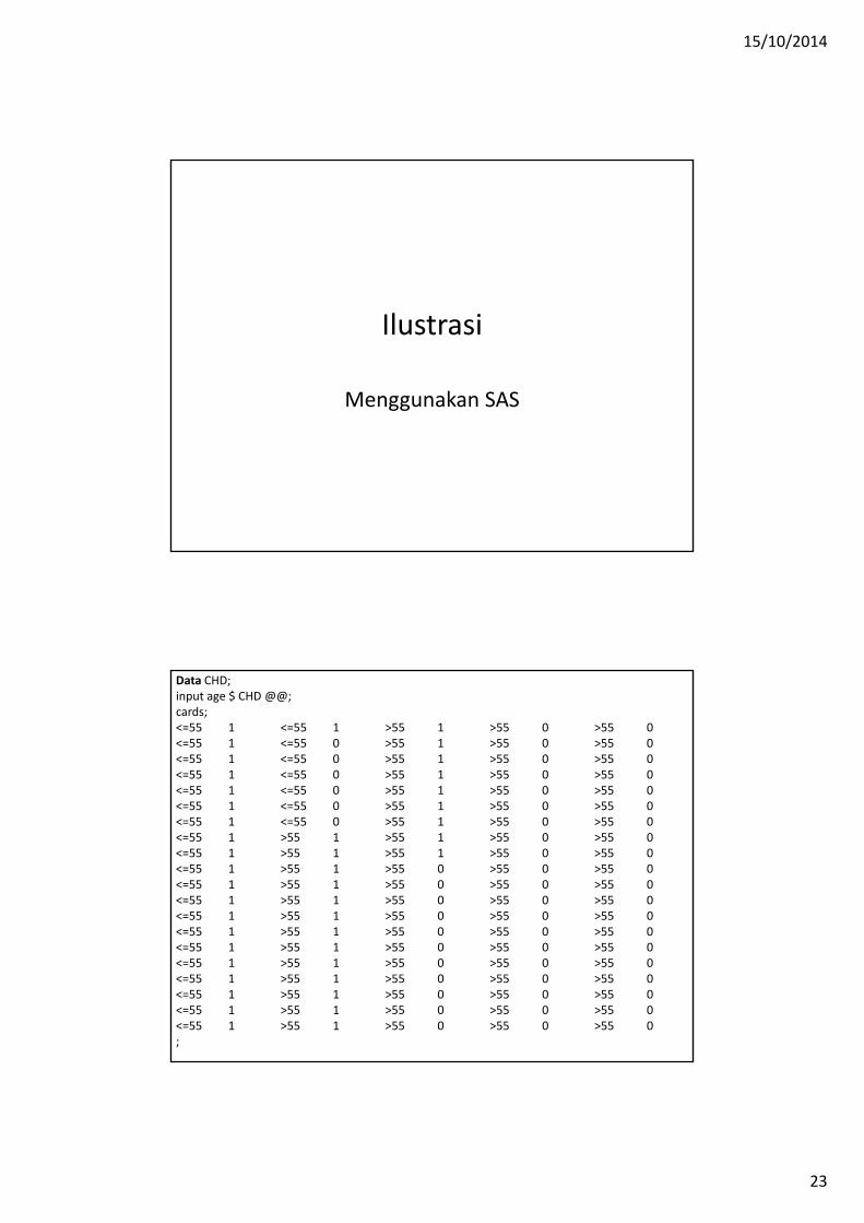
Ilustrasi 

Menggunakan SAS

Data CHD;input age $ CHD @@;cards;<=55 1 <=55 1 >55 1 >55 0 >55 0<=55 1 <=55 0 >55 1 >55 0 >55 0<=55 1 <=55 0 >55 1 >55 0 >55 0<=55 1 <=55 0 >55 1 >55 0 >55 0<=55 1 <=55 0 >55 1 >55 0 >55 0<=55 1 <=55 0 >55 1 >55 0 >55 0<=55 1 <=55 0 >55 1 >55 0 >55 0<=55 1 >55 1 >55 1 >55 0 >55 0<=55 1 >55 1 >55 1 >55 0 >55 0<=55 1 >55 1 >55 0 >55 0 >55 0<=55 1 >55 1 >55 0 >55 0 >55 0<=55 1 >55 1 >55 0 >55 0 >55 0<=55 1 >55 1 >55 0 >55 0 >55 0<=55 1 >55 1 >55 0 >55 0 >55 0<=55 1 >55 1 >55 0 >55 0 >55 0<=55 1 >55 1 >55 0 >55 0 >55 0<=55 1 >55 1 >55 0 >55 0 >55 0<=55 1 >55 1 >55 0 >55 0 >55 0<=55 1 >55 1 >55 0 >55 0 >55 0<=55 1 >55 1 >55 0 >55 0 >55 0<=55 1 >55 1 >55 0 >55 0 >55 0;

15/10/2014

24

proc freq data=CHD;tables age;tables CHD;tables age*CHD/nopercent nocol norowexpected chisq;run;

proc logistic data=CHD;class age;class age;model chd=age/expb;

run;

Tabulasi Silang

15/10/2014

25

Tugas Kelompok

Kelompok 1 Kelompok 2 (RegLog Berganda)

• Prediktor Kategorik• Uji Cochran‐Mantel 

Haenszel• Uji Kehomogenan Rasio 

Odd(Bab 4.3)

• Contoh Regresi Logistik Ganda

• Pembandingan Model(4.4.1, 4.4.2)

( )

15/10/2014

26

Tugas Kelompok (lanjutan)

Kelompok 3 (RegLog Berganda) Kelompok 4• Prediktor Kuantitatif dalam 

Regresi Logistik• Model dengan Interaksi(Bab 4.4.3, 4.4.4)

• Strategi Pemilihan Model• Pemeriksaan Kecocokan 

Model(Bab 5.1, 5.2)