arX

iv:1

710.

0902

2v2

[co

nd-m

at.s

tr-e

l] 7

Apr

201

8

Current transport properties and phase diagram of a Kitaev chain with long-range

pairing

Domenico Giuliano(1,2), Simone Paganelli(3), and Luca Lepori(3,4)(1) Dipartimento di Fisica, Universita della Calabria Arcavacata di Rende I-87036, Cosenza, Italy

(2) I.N.F.N., Gruppo collegato di Cosenza, Arcavacata di Rende I-87036, Cosenza, Italy(3) Dipartimento di Scienze Fisiche e Chimiche, Universita dell’ Aquila, via Vetoio, I-67010 Coppito-L’Aquila, Italy

(4) I.N.F.N., Laboratori Nazionali del Gran Sasso,Via G. Acitelli, 22, I-67100 Assergi (AQ), Italy

(Dated: April 10, 2018)

We describe a method to probe the quantum phase transition between the short-range topologicalphase and the long-range topological phase in the superconducting Kitaev chain with long-rangepairing, both exhibiting subgap modes localized at the edges. The method relies on the effects ofthe finite mass of the subgap edge modes in the long-range regime (which survives in the ther-modynamic limit) on the single-particle scattering coefficients through the chain connected to twonormal leads. Specifically, we show that, when the leads are biased at a voltage V with respect tothe superconducting chain, the Fano factor is either zero (in the short-range correlated phase) or 2e(in the long-range correlated phase). As a result, we find that the Fano factor works as a directlymeasurable quantity to probe the quantum phase transition between the two phases. In addition,we note a remarkable ”critical fractionalization effect” in the Fano factor, which is exactly equalto e along the quantum critical line. Finally, we note that a dual implementation of our proposeddevice makes it suitable as a generator of large-distance entangled two-particle states.

PACS numbers: 71.10.Pm , 73.21.-b , 74.78.Na , 74.45.+c .

I. INTRODUCTION

The Kitaev chain provides a prototypical example of a one-dimensional (1D) superconductive model with nontrivialtopology1. The related phase diagram consists of two gapped phases, separated by a quantum critical point (QCP),at which the mass gap closes and the system undergoes a phase transition between a topologically trivial and atopologically non trivial phase (TP). The hallmark of the emergence of the latter phase, which also constitutesits main point of interest, is the appearance of two unpaired real fermionic Majorana modes γL, γR (such that

γ†L/R = γ∗

L/R = γL/R), whose wave functions are localized at the endpoints of the chain2,3. This phenomenon is

strictly related to the spontaneous breaking of the Z2 fermion parity symmetry, due to the possibility of constructinga zero-energy Dirac mode d = 1

2 [γL + iγR] which, on acting over a generic energy eigenstate |E〉, changes its fermion

parity, without changing its energy4.Besides being interesting per se, the Kitaev Hamiltonian also maps onto the 1D Ising model in a transverse magnetic

field (TIM), by means of the standard Jordan-Wigner transformation (see for instance Ref.[5]). Therefore, it alsoprovides a way to exactly solve the 1D TIM by diagonalizing a quadratic fermion Hamiltonian. Along the Jordan-Wigner transformation, the fermion parity Z2 symmetry of the Kitaev Hamiltonian is traded for the spin-parity Z2

symmetry in the TIM. In particular, the topological phase in the former model corresponds to the ferromagneticphase in the latter6.Due to the remarkable emergence of a topological phase and to the relevance of Majorana modes as candidates for

working as fault-tolerant quantum bits7, the Kitaev chain has been largely studied in the last years. For instance,the effects on the Majorana modes of an additional electronic interaction along the chain have been considered inRef.[8], while the stability of a Majorana mode at the boundary of a Kitaev chain side coupled to an interactingnormal wire has been discussed in Refs.[9,10]. Devices in which two Kitaev chains are connected to each other viaa normal central region in an NSN-Josephson junction arrangement have been discussed as well in Ref.[11], wherea particular focus has been put on the effects of the Majorana modes on the Josephson current flowing across thewhole NSN junction when a fixed phase difference between the two superconductors is applied. Junctions of Kitaevchains have also been studied as a natural arena to realize and manipulate Majorana modes in a controlled way12,as well as an equivalent model (via the Jordan-Wigner transformation) of junctions of quantum spin chains13–16, orof suitably designed Josephson junction networks17,18. On the experimental side, the Kitaev chain has been arguedto provide an effective description of a superconducting proximity-induced 1D quantum wire with strong spin-orbitcoupling and Zeeman effect12,19, which has accordingly been proposed as a feasible arena to experimentally lookfor emerging Majorana modes. Indeed, following this scheme, the Kitaev chain has been experimentally realized insuitably designed devices20,21.The above mentioned remarkable features of the Kitaev Hamiltonian have recently triggered considerable interest

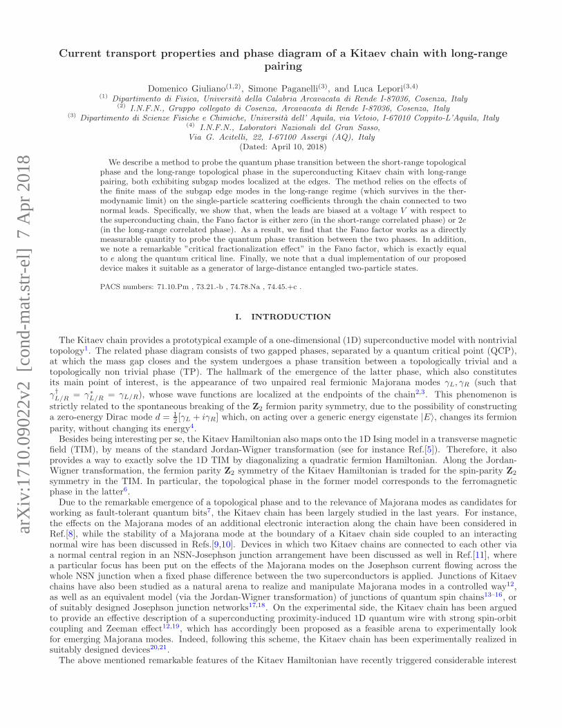
2

FIG. 1: Phase diagram of the LRK chain in the α-µ plane: The various phases are characterized by different values of theBerry phase γ (see main text for details)

in generalizations of it, with possible additional novel phases. In this direction, a particularly interesting example isprovided by the Kitaev chain with long-range pairing (LRK)22,23, with generalizations to long-range hopping24,25 andto Ising chains with long-range magnetic exchange strength24,26,27, as well as to higher-dimensional Hamiltonians28,29

(it is also worth mentioning the possibility of driving topological phase transitions by means of non-Abelian gaugepotentials in optical lattices30). The LRK is defined as a generalization of the Kitaev chain, with the pairing betweenparticles at sites i and j decaying by a power-law function ∼ |i− j|−α, α ≥ 0. The standard Kitaev Hamiltonian, withpairing involving only nearest-neighboring sites, is recovered in the limit α → ∞. On the experimental side, recentproposals have been put forward to realize the LRK and its generalizations by a Floquet engineering via an appliedexternal AC field31–33, using neutral atoms loaded onto an optical lattice coupled to photonic modes34–40, or usingShiba bound states induced in a chain of magnetic impurities on the top of an s-wave superconductor41,42.As the LRK, either with short-range or with long-range pairing, is described by a quadratic fermion Hamiltonian, it

can be exactly solved within the standard approach to noninteracting fermion problems43. This allowed for mappingout the whole phase diagram in the µ−α plane (µ being the chemical potential), displayed in Fig. 1. As a result, twonew phases have been found out22–25,27, not continuously connected to those characterizing the Kitaev model in theshort range limit1. These phases have been also inferred, not included in the classification of topological insulatorsand superconductors valid in the short-range limit44–46. They are suggested and characterized by:

• The appearance of noninteger winding numbers at α < 125,27. This property, as well as the ones describedabove, can be ascribed to the divergencies developing in the quasiparticle spectrum for those values of α23,27.Equivalently, a pertinently defined Berry phase γ here takes the values γ = ± π/2 (at µ ≷ 1), different from thevalues γ = 0, π, which label the phases of the Kitaev chain with short range pairing.

• The emergence of subgap modes localized at the edges of the open chain in the phase at α < 1 and µ < 1,as a remnant of the edge modes in the phase at α > 1 and |µ| < 1. In the latter case, the structure of thesesubgap modes is qualitatively equivalent to those in the Kitaev model: Two real fermionic modes emerge, withwave functions localized at the endpoints of the chain, which eventually evolve into the Majorana modes withvanishing mass in the infinite-chain limit. The emergence of the Majorana modes induces the spontaneousbreaking of the fermion parity Z2 symmetry and it is the hallmark of the onset of a topological phase46 (this”short-range topological” phase will be denoted in the following as SRTP).On the contrary, for α < 1, there are still subgap modes with wave functions mostly localized around theendpoints of the chain, but with the corresponding wave function overlap keeping finite, even in the infinite-chain limit. This corresponds to the onset, in the same limit and at µ < 1, of a subgap mode with nonvanishingmass, determined by the hybridization of the two Majorana modes emerging at α > 124,47. Such phenomenonleads to a nondegenerate groundstate, thus restoring the Z2-symmetry. This restore is by itself sufficient toevidence the emergence at µ < 1 and α < 1 of a phase not continuously connected to the topological phase ofthe standard (short-range) Kitaev model.

• The violation of the area law for the Von Neumann entropy48, also in the gapped regions, as soon as α < 122,23,49,and for every value of µ. On the contrary, the area law is respected ∀α > 1. The mentioned violation has beenshown49 to be deeply related to the singularities in the quasiparticle spectrum, originating the noninteger windingnumbers.

3

The long-range correlated phase at µ < 1 and α < 1 is also characterized by a suitably defined nontrivial LRtopology27, indeed reflecting in the massive subgap edge states. For this reason, the same phase will be denoted asLRTP in the following. Finally, a quantum phase transition at α = 1, not first order (following the Ehrenfest scheme)22

and without any mass gap closure, can be inferred, also falling outside the standard schemes for the classificationof quantum phases transitions, as presented in detail in, e.g., Ref.[50]. This result can be achieved mainly by otherspecific features, such as those listed above, and the divergence of the fidelity susceptibility51 in α along the lineα = 152.In this paper we focus mainly on the SRTP and LRTP, characterized by the presence of subgap edge modes, and

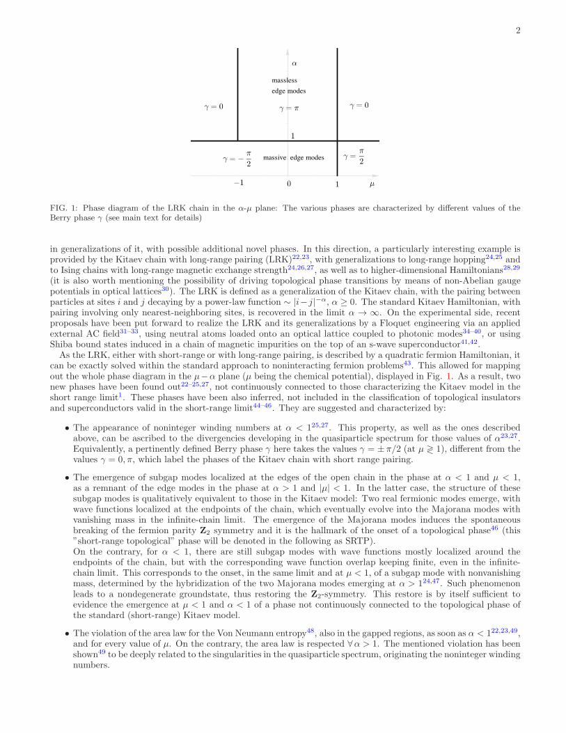
on the quantum phase transition between the two of them. In particular, we discuss how the emergence of themassive subgap edge modes, signaling the onset of the LRTP at α < 1 and µ < 1, affects the single-particle scatteringcoefficients across the LRK, when it is connected to two normal leads, from which particles and/or holes are injectedinto the LRK and collected after scattering. Specifically, we discuss an NSN device, in which the LRK is the centralsuperconducting region, and the normal leads at its side can be biased to a finite voltage V with respect to this region,so to make an electric current flow across the SN interfaces. In fact, our system, sketched in Fig. 2, can be regardedas an adapted version of the NSN junction studied in Ref.[53] to discuss nonlocal Andreev reflection processes. Torealize our device, one needs a solid-state realization of the LRK Hamiltonian which can be recovered, for instance,as in Refs.[41,42], that is, by using helical Shiba states emerging at a chain of magnetic impurities deposited on topof an s-wave superconducting substrate. The level of control one may achieve in a system as such allows, in principle,to tunnel couple the chain of magnetic impurities to normal contacts, which can be biased at a voltage V and, at thesame time, can be used to probe electric transport across the emerging LRK. Varying the superconducting coherencelength of the host superconductor at a fixed length of the chain, one may also change the effective range of the inducedpairing, so to make the system crossover from an effectively short-range pairing regime to a long-range pairing one.Note that keeping finite the length of the chain does not constitute an obstruction for the emergence of long-rangephysics, as described in detail in Ref.[27].The key idea is that, when the leads are weakly coupled to the LRK in the SRTP, as ℓ grows, the low-energy (subgap)

scattering processes across the NSN junction are expected to be fully determined by the two uncorrelated Majoranamodes residing at the SN interfaces. As it happens with the Kitaev Hamiltonian, this implies at the Fermi energy ofthe leads a strong suppression of all the scattering processes across each SN interface but the (local) Andreev reflection(LAR), consisting in the injection of a Cooper pair in the superconductive region, via the absorption of a particlefrom the injecting lead and in the creation in the same lead of a counter propagating hole54, whose correspondingscattering coefficient flows to 111,55. Instead, when the system lies within the LRTP, the finite hybridization betweenthe Majorana modes, yielding the massive subgap edge modes, is rather expected to lead to a full suppression of LAR,while keeping alive all the other scattering processes, including the remarkable nonlocal ”crossed Andreev reflection”(CAR) across the LRK, in which, differently from the LAR, the hole injected at one SN interface of the NSN systemeventually emerges as a particle at the opposite interface53, with the corresponding scattering coefficients that keepfinite at the Fermi energy.Both LAR and CAR can make a finite current flowing across the SN interfaces when the leads are biased at a

finite voltage V with respect to the LRK. Nevertheless, as argued in Ref.[53], a combined measurement of the currentand of the zero-frequency current noise is able to discriminate whether it is the LAR or the CAR the process that iseffective in supporting the (low-V ) current flow.Using this method, we look at the Fano factor, that is, at the ratio between the current noise and the current itself

as V → 0. We show that, whenever the current is supported by LAR (that is within the SRTP), the Fano factorflows to 0 as V → 0, while, when the current is supported by CAR (that is within the LRTP), the Fano factor flowsto 2e in the same limit, keeping equal to e exactly at the phase transition line (α = 1). Thus, on one hand we designa possible experiment to discriminate between the two phases by means of a simple transport measurement. On theother hand, by considering a possible experiment based on a process ”dual” to CAR, in which one imagines to injecta Cooper pair from the superconductor into the leads as two outgoing particles, we argue how the LRTP can bein principle used to create pairs of distant (in real space), highly-entangled particles. To witness the reliability ofthe combined measurements of current and noise to evidence the emergence of subgap modes in hybrid structures,it is worth stressing that it has been proposed to detect Majorana fermions at the edge of a vortex core in a chiral(two-dimensional) p-wave superconductor56, to probe Majorana modes at the interface between a superconductorand (the surface of) a topological insulator57, or in a Majorana fermion chain58, to measure Majorana fermions viatransport through a quantum dot59.In our case, while we acknowledge the difficulty of realizing our proposed NSN junction in a real solid-state device

and of tuning α across the quantum critical line α = 1, we believe that the experimental techniques mentioned abovecan make it possible to realize soon the junction in a controllable way.The paper is organized as follows:

• In Sec. II we introduce the model Hamiltonian for the NSN junction with the S-region realized by the 1D LRK

4

IL

L−lead R−leadLRK

V

IR

FIG. 2: Sketch of the NSN junction that we discuss in the paper. A LRK works as the central region of the junction; thisregion is connected to two normal leads, which can be biased at a finite voltage V with respect to the LRK, thus making thecurrents IL and IR, respectively, flow through the left-hand and the right-hand SN interfaces. This is an adapted version ofthe device proposed in Ref.[53].

and review some basic features of the latter model. We then compute the single-particle/single-hole scatteringamplitudes across the LRK, as a function of the energy E (measured with respect to the Fermi level of theleads) of the incoming particle/hole, paying particular attention to the E → 0-limit.

• In Sec. III we compute the current flowing through the leads when they are biased at a finite voltage V withrespect to the superconducting central region. We then compute the corresponding zero-frequency noise andthe Fano factor within both the SRTP and the LRTP, highlighting the different behavior of the various physicalquantities (currents and shot noise) in the two phases.

• In Sec. IV we discuss the current, the noise and the Fano factor across the quantum phase transition line atα = 1.

• In Sec, V we provide some concluding remarks and possible further developments of our work; then we discussa possible solid-state implementation of the LRK.

Mathematical details concerning the calculations of the physically relevant quantities are provided in the appendices.In particular, in Appendix C we prove how our formalism (based on an extensive use of single-particle Green’sfunctions to compute the various scattering amplitudes) is able to provide us back with the results of Ref.[53] in theℓ = 1 limit.

II. MODEL HAMILTONIAN AND SINGLE-PARTICLE SCATTERING PROCESSES

In this section we introduce our main model Hamiltonian, discuss how we recover the scattering amplitudes withinthe imaginary time Green’s function framework, discuss our results for the scattering coefficients, and compare themto the ones obtained within a simplified model adapted from Ref.[53].

A. The model Hamiltonian

Throughout this paper, we consider the LRK as a reference model since. As studied and discussed in Refs.[23,24],models characterized by a long-range hopping amplitude, as well, do not give rise to qualitative modifications in thephase diagram. The corresponding LRK over an ℓ-site lattice reads22

HLR = −w

ℓ−1∑

j=1

d†jdj+1 + d†j+1dj − µ

ℓ∑

j=1

d†jdj +∆

2

ℓ−1∑

j=1

ℓ−1∑

r=1

δ−αr djdj+r + d†j+rd

†j , (1)

with dj , d†j being lattice fermion operators and δr = |r| whenever j + r ≤ ℓ, otherwise δr = 0. HLR in Eq.(1) is a

generalization of the (short-range) Kitaev Hamiltonian1, to which it reduces as α → ∞. In the following, without anyloss of generality, we conventionally choose the parameters of HLR in analogy to what is done in22: ∆ = 2w = 1.

5

Incidentally, we note that, while for nearest-neighbor pairing, the Hamiltonian in Eq.(1) naturally emerges whenconsidering the Jordan-Wigner representation of the one-dimensional Ising model in a transverse magnetic field, sucha correspondence does not extend to the long-range Ising chain, due to the absence of cancellations between the Diracstrings in the Jordan-Wigner representation of the spin operators24; indeed, this makes it not possible to solve thelong-range Ising chain via the solution of the LRK.In Fig. 1, we show the phase diagram of the Hamiltonian in Eq.(1) in the µ and α plane. In the limit α → ∞, on

varying µ, two topological phase transitions are expected to take place at µ = ±1, with the topologically nontrivialphase, where the Majorana modes γL and γR appear at the endpoints of the open chain, realized when |µ| < 1. Withinthe same interval of values of µ, but at α < 1, the LRTP phase sets in, characterized by a finite hybridization energyǫd between the two edge modes24,47, which keeps finite in the thermodynamic limit and is typically accompanied bythe onset of a purely algebraic decay of the corresponding real-space wave functions22,24.In order to discriminate between the two phases by means of an appropriate scattering experiment, we let particles

and holes to be shot from the side reservoirs (leads) against the central region. We model the normal leads by meansof noninteracting spinless fermion Hamiltonians HLead =

∑

X=L,R HX , with

HL = −J∑

j≤−1

c†L,jcL,j+1 + c†L,j+1cL,j − µ′∑

j≤0

c†L,jcL,j

HR = −J∑

j≥ℓ+1

c†R,jcR,j+1 + c†R,j+1cR,j − µ′∑

j≥ℓ+1

c†R,jcR,j , (2)

cR/L,j being single-fermion operators over each lead, J and µ′ the corresponding hopping amplitude and chemicalpotential, and, by convention, j ≤ 0 for the left-hand lead and j ≥ ℓ + 1 for the right-hand lead. Finally, we modelthe coupling between the central superconductive region and the leads by means of the tunneling Hamiltonian

HT = −tc†L,0d1 + d†1cL,0 − tc†R,ℓ+1dℓ + d†ℓcR,ℓ+1 . (3)

We remark that, using HT as tunneling operator is equivalent to assuming purely local tunneling between S and theleads, despite intrinsically long-range nature of the correlations in S. This is justified by making a weak couplingassumption between S and the leads, that is, t/J ≪ 1. Finally, we note that, to simplify the derivation, we havechosen the lead Hamiltonian parameters in Eq.(2), as well as the hopping amplitudes in Eq.(3), L − R-symmetric,since the results are qualitatively equivalent to what one gets assuming different Hamiltonian parameters in HR andHL and/or different hopping amplitudes in HT .

B. The strategy to derive the scattering amplitudes

Scattering through the NSN junction is fully encoded the one-particle S matrix53,60 S(E), E being the energy of theincoming particle from the leads at the beginning of the scattering process, measured with respect to the Fermi level ofthe leads. To set up the notation, in the following we denote with rX,X(E) (rX,X(E)) the normal backscattering (NB)amplitude for a particle (hole) incoming from the lead X , with aX,X(E) (aX,X(E)) the LAR amplitude for a particle(hole) incoming from the lead X , with tX,X′(E) (tX,X′(E)) the normal transmission (NT) amplitude for a particle(hole) incoming from the lead X into the lead X ′ 6= X and, finally, with cX,X′(E) (cX,X′(E)) the CAR amplitude fora particle (hole) incoming from the lead X into the lead X ′. All the scattering amplitudes appear as entries of theS-matrix, which provides the outgoing state on pertinently acting onto the incoming state. In the low-energy limitin which one can assume that the particle- and hole-velocities are equal to each other and both equal to the Fermivelocity v, the S matrix is given by

S(E) =

rL,L(E) aL,L(E) tL,R(E) cL,R(E)aL,L(E) rL,L(E) cL,R(E) tL,R(E)tR,L(E) cR,L(E) rR,R(E) aR,R(E)cR,L(E) tR,L(E) aR,R(E) rR,R(E)

. (4)

Typically, for a quadratic Hamiltonian such as HLR, one may in principle construct S(E) by solving the Bogoliubov-de Gennes (BDG) equations for the lattice energy eigenfunctions in the scattering basis, whose elements are labeledaccording to whether the incoming state corresponds to a particle or a hole, coming from the left-hand, or from theright-hand lead61,62. While this procedure might in principle be applied to our system as well, by using the basis ofscattering states that we review in Appendix B 1, in fact, due to the long-range pairing term in HLR, the continuityconditions at the SN interfaces become quite hard to deal with.

6

For this reason, we resort to an alternative method63, based on the relation between the fully dressed Green’sfunction of the NSN junction (which we exactly compute in Appendix A) and the S matrix, which we review indetail in Appendix B. Specifically, we first use the equations of motion, as implemented in Appendix B, to prove thatS(E) basically depends on the Green’s function of the central region, Gd;(j,j′)(E), j, j′ ∈ 1, ℓ. Then, in order tooptimize the numerical calculation, we resort to imaginary time formalism, eventually computing the Green’s functionover the imaginary axis in frequency space, Gd;(j,j′)(iω). Finally, to recover the scattering amplitudes over the real

axis, we analytically continue Gd;(j,j′)(iω) for ω > 0, by means of the substitution iω → E + i0+. To perform thecalculation, we numerically diagonalize HLR at finite-ℓ for different values of µ and α and use the resulting eigenvaluesand eigenvectors to construct Gd;(j,j′)(iω). The relation between S(E) and Gd;(j,j′)(iω → E + i0+) is readily derivedby combining Eqs. (B18) of Appendix B with Eqs. (A13, A14, A15, A16) of Appendix A2.

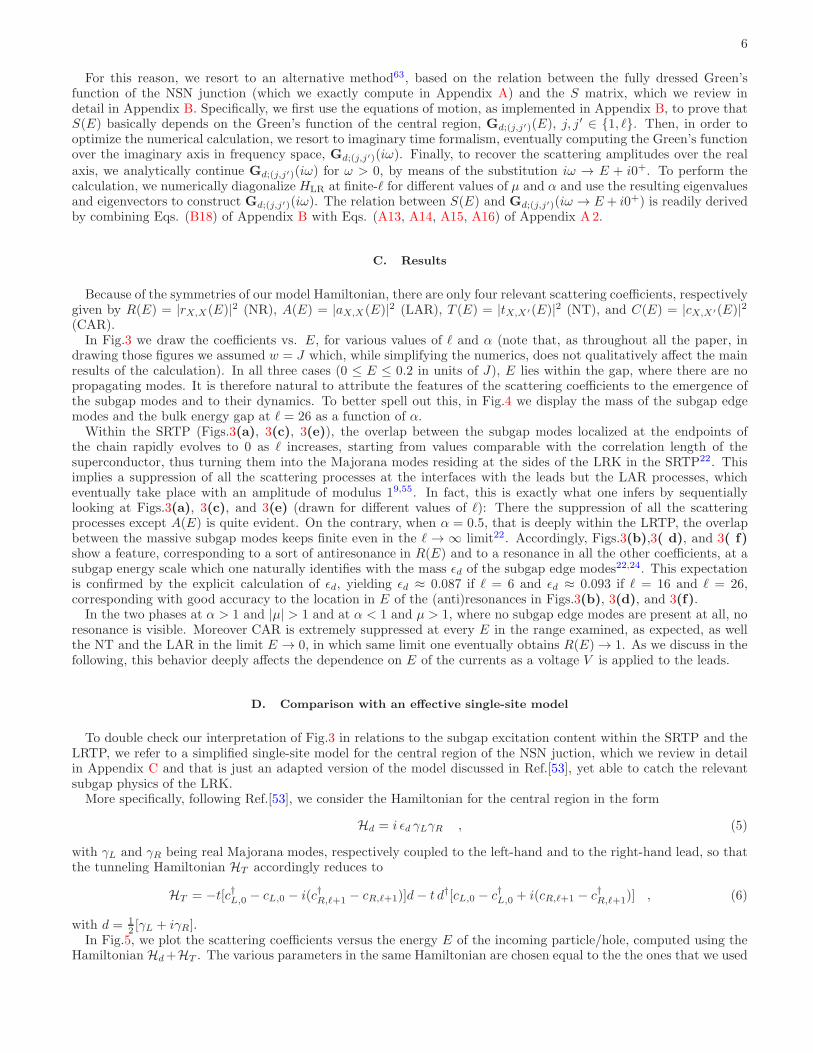
C. Results

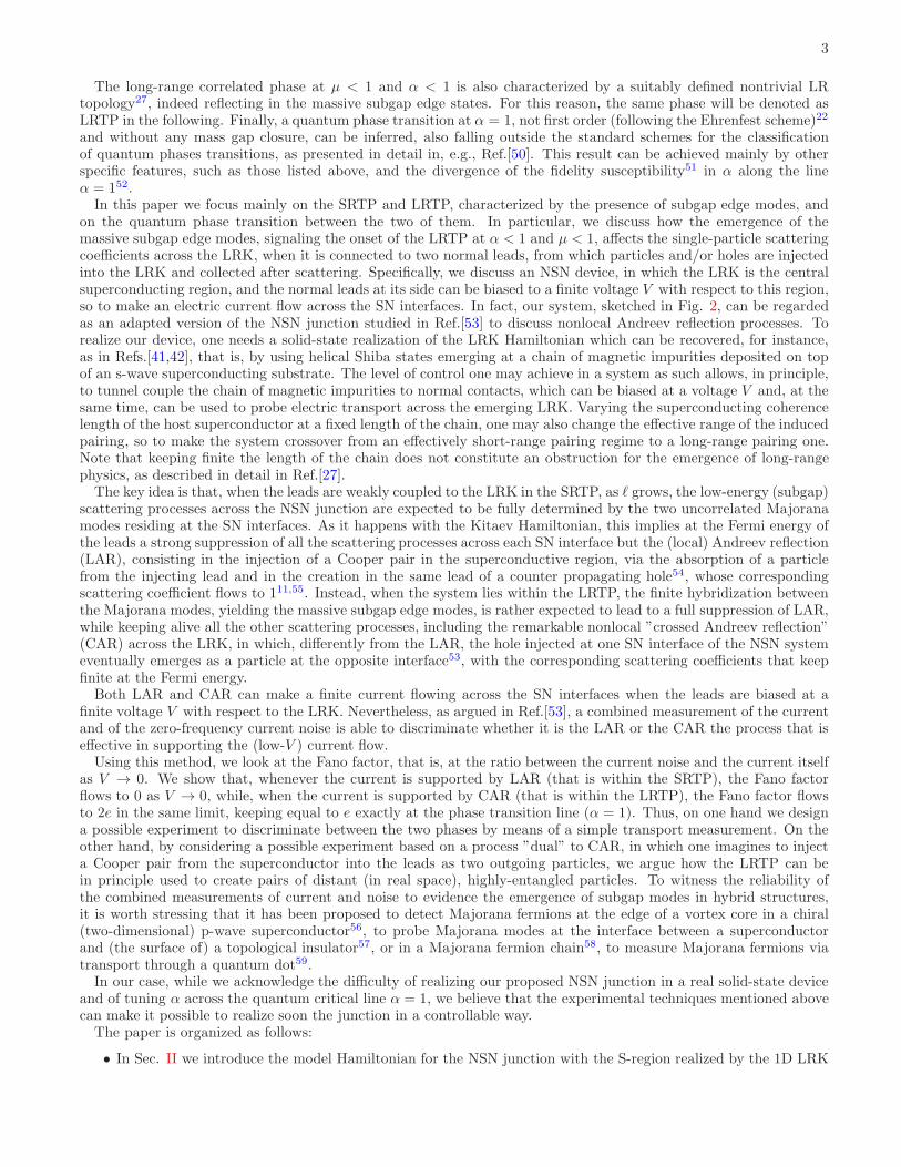
Because of the symmetries of our model Hamiltonian, there are only four relevant scattering coefficients, respectivelygiven by R(E) = |rX,X(E)|2 (NR), A(E) = |aX,X(E)|2 (LAR), T (E) = |tX,X′(E)|2 (NT), and C(E) = |cX,X′(E)|2

(CAR).In Fig.3 we draw the coefficients vs. E, for various values of ℓ and α (note that, as throughout all the paper, in

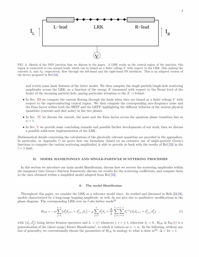
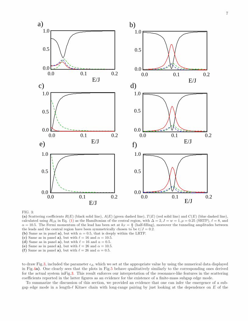
drawing those figures we assumed w = J which, while simplifying the numerics, does not qualitatively affect the mainresults of the calculation). In all three cases (0 ≤ E ≤ 0.2 in units of J), E lies within the gap, where there are nopropagating modes. It is therefore natural to attribute the features of the scattering coefficients to the emergence ofthe subgap modes and to their dynamics. To better spell out this, in Fig.4 we display the mass of the subgap edgemodes and the bulk energy gap at ℓ = 26 as a function of α.Within the SRTP (Figs.3(a), 3(c), 3(e)), the overlap between the subgap modes localized at the endpoints of

the chain rapidly evolves to 0 as ℓ increases, starting from values comparable with the correlation length of thesuperconductor, thus turning them into the Majorana modes residing at the sides of the LRK in the SRTP22. Thisimplies a suppression of all the scattering processes at the interfaces with the leads but the LAR processes, whicheventually take place with an amplitude of modulus 19,55. In fact, this is exactly what one infers by sequentiallylooking at Figs.3(a), 3(c), and 3(e) (drawn for different values of ℓ): There the suppression of all the scatteringprocesses except A(E) is quite evident. On the contrary, when α = 0.5, that is deeply within the LRTP, the overlapbetween the massive subgap modes keeps finite even in the ℓ → ∞ limit22. Accordingly, Figs.3(b),3( d), and 3( f)show a feature, corresponding to a sort of antiresonance in R(E) and to a resonance in all the other coefficients, at asubgap energy scale which one naturally identifies with the mass ǫd of the subgap edge modes22,24. This expectationis confirmed by the explicit calculation of ǫd, yielding ǫd ≈ 0.087 if ℓ = 6 and ǫd ≈ 0.093 if ℓ = 16 and ℓ = 26,corresponding with good accuracy to the location in E of the (anti)resonances in Figs.3(b), 3(d), and 3(f).In the two phases at α > 1 and |µ| > 1 and at α < 1 and µ > 1, where no subgap edge modes are present at all, no

resonance is visible. Moreover CAR is extremely suppressed at every E in the range examined, as expected, as wellthe NT and the LAR in the limit E → 0, in which same limit one eventually obtains R(E) → 1. As we discuss in thefollowing, this behavior deeply affects the dependence on E of the currents as a voltage V is applied to the leads.

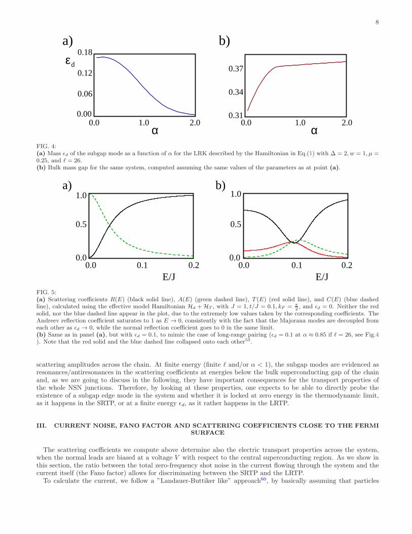
D. Comparison with an effective single-site model

To double check our interpretation of Fig.3 in relations to the subgap excitation content within the SRTP and theLRTP, we refer to a simplified single-site model for the central region of the NSN juction, which we review in detailin Appendix C and that is just an adapted version of the model discussed in Ref.[53], yet able to catch the relevantsubgap physics of the LRK.More specifically, following Ref.[53], we consider the Hamiltonian for the central region in the form

Hd = i ǫd γLγR , (5)

with γL and γR being real Majorana modes, respectively coupled to the left-hand and to the right-hand lead, so thatthe tunneling Hamiltonian HT accordingly reduces to

HT = −t[c†L,0 − cL,0 − i(c†R,ℓ+1 − cR,ℓ+1)]d− t d†[cL,0 − c†L,0 + i(cR,ℓ+1 − c†R,ℓ+1)] , (6)

with d = 12 [γL + iγR].

In Fig.5, we plot the scattering coefficients versus the energy E of the incoming particle/hole, computed using theHamiltonian Hd+HT . The various parameters in the same Hamiltonian are chosen equal to the the ones that we used

7

b)

E/J

E/J

a)

E/Jc)

E/JE/J

d)

E/J

f)e)

1.0

0.5

0.0 0.0 0.2 0.1

1.0

0.5

0.0 0.0 0.1 0.2

1.0

0.5

0.0 0.1 0.0 0.2

0.1 0.2 0.0 0.0

1.0

0.5

0.2 0.1 0.0 0.0

1.0

0.5

1.0

0.0 0.2 0.0

0.5

0.1

FIG. 3:(a) Scattering coefficients R(E) (black solid line), A(E) (green dashed line), T (E) (red solid line) and C(E) (blue dashed line),calculated using HLR in Eq. (1) as the Hamiltonian of the central region, with ∆ = 2, J = w = 1, µ = 0.25 (SRTP), ℓ = 8, andα = 10.5. The Fermi momentum of the lead has been set at kF = π

2(half-filling), moreover the tunneling amplitudes between

the leads and the central region have been symmetrically chosen to be t/J = 0.2.(b) Same as in panel a), but with α = 0.5, that is deeply within the LRTP.(c) Same as in panel a), but with ℓ = 16 and α = 10.5.(d) Same as in panel a), but with ℓ = 16 and α = 0.5.(e) Same as in panel a), but with ℓ = 26 and α = 10.5.(f) Same as in panel a), but with ℓ = 26 and α = 0.5.

to draw Fig.3, included the parameter ǫd, which we set at the appropriate value by using the numerical data displayedin Fig.4a). One clearly sees that the plots in Fig.5 behave qualitatively similarly to the corresponding ones derivedfor the actual system inFig.3. This result enforces our interpretation of the resonance-like features in the scatteringcoefficients reported in the latter figures as an evidence for the existence of a finite-mass subgap edge mode.To summarize the discussion of this section, we provided an evidence that one can infer the emergence of a sub-

gap edge mode in a length-ℓ Kitaev chain with long-range pairing by just looking at the dependence on E of the

8

εd

α α

a) b)

0.06

0.12

0.18

0.0 1.0 2.0 0.00 0.31

0.34

0.37

2.0 0.0 1.0

FIG. 4:(a) Mass ǫd of the subgap mode as a function of α for the LRK described by the Hamiltonian in Eq.(1) with ∆ = 2, w = 1, µ =0.25, and ℓ = 26.(b) Bulk mass gap for the same system, computed assuming the same values of the parameters as at point (a).

E/JE/J

b)a)

0.0 0.1 0.2 0.0

0.5

1.0

0.0

1.0

0.5

0.0 0.1 0.2

FIG. 5:(a) Scattering coefficients R(E) (black solid line), A(E) (green dashed line), T (E) (red solid line), and C(E) (blue dashedline), calculated using the effective model Hamiltonian Hd +HT , with J = 1, t/J = 0.1, kF = π

2, and ǫd = 0. Neither the red

solid, nor the blue dashed line appear in the plot, due to the extremely low values taken by the corresponding coefficients. TheAndreev reflection coefficient saturates to 1 as E → 0, consistently with the fact that the Majorana modes are decoupled fromeach other as ǫd → 0, while the normal reflection coefficient goes to 0 in the same limit.(b) Same as in panel (a), but with ǫd = 0.1, to mimic the case of long-range pairing (ǫd = 0.1 at α ≈ 0.85 if ℓ = 26, see Fig.4). Note that the red solid and the blue dashed line collapsed onto each other53.

scattering amplitudes across the chain. At finite energy (finite ℓ and/or α < 1), the subgap modes are evidenced asresonances/antiresonances in the scattering coefficients at energies below the bulk superconducting gap of the chainand, as we are going to discuss in the following, they have important consequences for the transport properties ofthe whole NSN junctions. Therefore, by looking at these properties, one expects to be able to directly probe theexistence of a subgap edge mode in the system and whether it is locked at zero energy in the thermodynamic limit,as it happens in the SRTP, or at a finite energy ǫd, as it rather happens in the LRTP.

III. CURRENT NOISE, FANO FACTOR AND SCATTERING COEFFICIENTS CLOSE TO THE FERMISURFACE

The scattering coefficients we compute above determine also the electric transport properties across the system,when the normal leads are biased at a voltage V with respect to the central superconducting region. As we show inthis section, the ratio between the total zero-frequency shot noise in the current flowing through the system and thecurrent itself (the Fano factor) allows for discriminating between the SRTP and the LRTP.To calculate the current, we follow a ”Landauer-Buttiker like” approach60, by basically assuming that particles

9

and holes are shot into the junction from thermal reservoirs at temperature T (which we eventually send to 0, so torecover the shot-noise regime, that is, kBT ≪ eV , with kB being the Boltzmann constant).The main derivation of the formulas for the currents and for the current correlations is summarized in Appendix

D, where we also show that the current flowing across the left- and right-hand lead, (IL and IR, respectively) is givenby IL = −IR = I, with

I =2e

2π

∫ ∞

0

dE f(−E − eV )− f(−E + eV ) |aL,L(E)|2 + |cL,R(E)|2 , (7)

f(E) being the Fermi distribution function at the temperature T of the thermal reservoirs, while aL,L(E) and cL,R(E)are the amplitudes for the (local and crossed) Andreev reflection, defined in Sec. II B. At zero temperature (and,more generally, in the shot-noise regime), Eq.(7) becomes

I =2e

2π

∫ eV

0

dE |aL,L(E)|2 + |cL,R(E)|2 . (8)

Equations (7) and (8) clearly show that a nonzero net current may flow toward the leads even for eV smaller thanthe superconducting gap of the central region, provided that either the LAR amplitudes, or the CAR amplitudes (orboth of them) keep different from zero close to the Fermi energy. Incidentally, this implies a strong suppression of thesubgap electric transport within the non-topological phase at µ > 1 and α > 1, where, as described in Sec. II C, allthe scattering amplitudes but the ones corresponding to normal reflection processes go to zero when approaching theFermi level, E → 0 . The same suppression occurs at α < 1 if µ > 1 and no massive subgap modes are present.As a special case of Eqs.(7) and (8), one may consider the limit of zero CAR amplitude, cL,R(E → 0) → 0. When

accompanied by a suppression of the normal transmission amplitude as well [tL,R(E → 0) → 0], this limiting situationmimics what happens at a single NS interface, where the finite-temperature (zero-temperature) current is given byEq.(7) [Eq.(8)], with cL,R(E) = 061,62. In the specific case of a LRK within the SRTP at α > 1, the emergence of theMajorana mode suppresses all the backscattering processes, except the LAR. This partial suppression makes the DCconductance G, associated to the current transport through the normal region, reach the maximum consistent with

unitarity constraint with an elementary carrier charge e∗ = 2e, that is, G = 2e2

2π9,10.

In our specific case, as we see from the plots of the previous section within the SRTP and the LRTP, either aL,L(E)or cL,R(E) (or both) keep nonvanishing as E → 0, which makes it hard to disentangle, from a measurement yielding afinite I at low values of eV , whether to attribute it to LAR or to CAR and, accordingly, whether to attribute a finitevalue of I to the onset of the SRTP or of the LRTP. Therefore, in order to define an experimental mean to distinguishthe two phases from each other via transport measurements, we follow the approach of Refs.[53,56,57] and considerthe zero-frequency shot noise associated to I.In order to evidence the L − R symmetry in the formula for the shot noise, we use a symmetrized version of the

operator associated to I, given by J = 12Jj − Jj′, with j belonging to lead L and j′ to lead R and

Jj = −ieJc†jcj+1 − c†j+1cj . (9)

For eV ≫ kBT , we obtain

I = 〈J(t)〉 =e

2π

∫ eV

0

dE |aL,L(E)|2 + |aR,R(E)|2 + |cL,R(E)|2 + |cR,L(E)|2 , (10)

with 〈. . .〉 denoting the thermal average with respect to the lead distribution functions. On applying the definition ofthe shot noise to our specific system, we find that the zero-frequency shot noise associated to J at a voltage bias V ,P(0, V ) is given by

P(0, V ) =1

4PL,L(0, V ) + PR,R(0, V )− PL,R(0, V )− PR,L(0, V ) , (11)

with PL,L(0), PR,R(0) , PL,R(0), PR,L(0), defined in Eqs.(D9,D10,D11,D12) of Appendix D 2 as combinations of thescattering amplitudes appearing in the S(E) matrix in Eq.(4) (for notational simplicity, in the following we will notexplicitly show the dependence of the shot noise on the voltage V ).The key quantity we now look at is the Fano factor, defined as P(0)/I. Within the SRTP, in the eV → 0 limit,

all the scattering coefficients but the LAR one are suppressed. This makes the SN junctions behave as a perfect

conductor, with conductance equal to G = 2e2

2π9,10 and with a corresponding suppression of the zero-frequency shot-

noise; therefore the Fano factor is expected to flow to 0 as e V → 0. On the contrary, within the LRTP, we infer

10

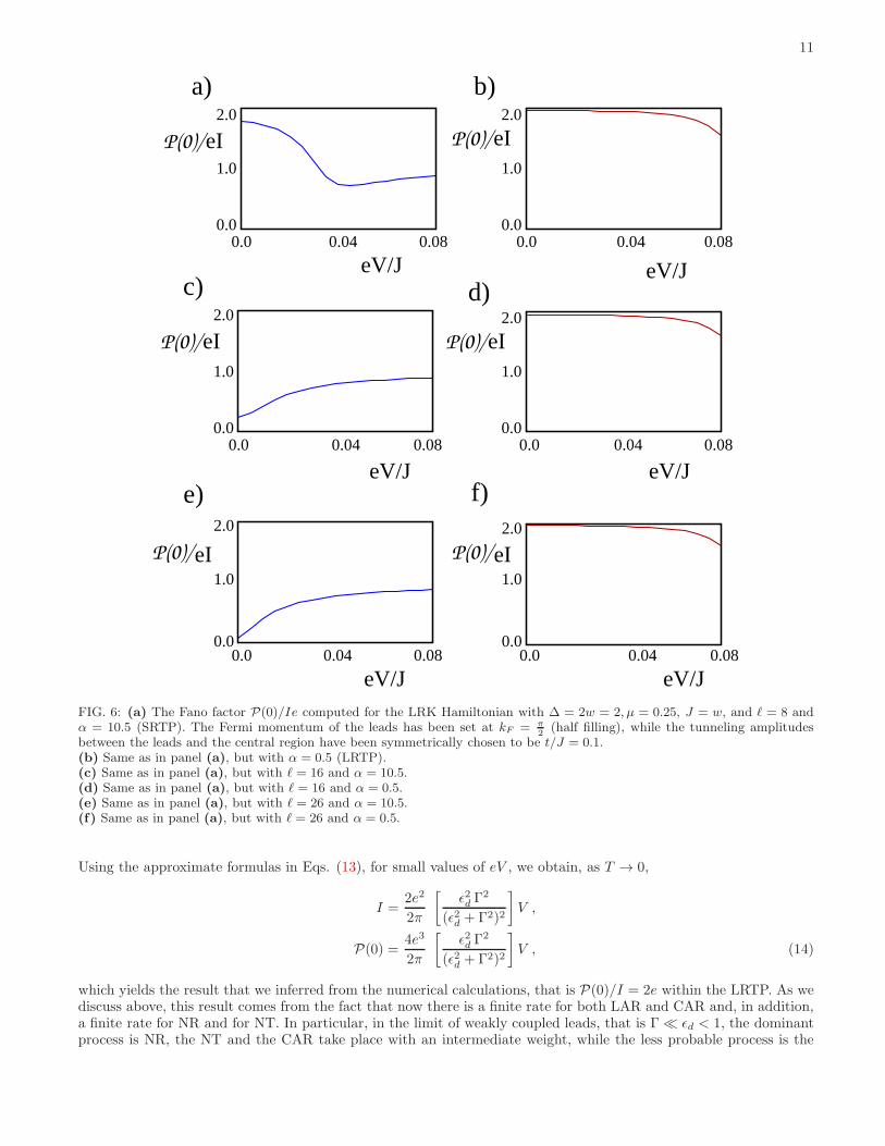
from the plots in Figs.3(b), 3( d), 3(f) that, though reduced, both the CAR and the LAR coefficients keep finite aseV → 0, due to the emergence of the finite-energy massive subgap modes. In addition, also the NR and NT scatteringcoefficients keep finite as well when eV → 0. While this is already enough to expect a nonzero Fano factor as eV → 0,we also note that, in the limit in which the leads are weakly coupled to the LRK (that is, at small values of t/J), thephysical processes supporting the current transport across the NSN junction become rare events. These processes areexactly the LAR and the CAR, plus complementary processes obtained from the symmetries of the S matrix. Sincethe net charge of the elementary charge carrier is e∗ = 2e (that is, the charge of a Cooper pair), we expect on onehand that the zero-frequency shot noise becomes Poissonian, on the other hand that, as eV → 0, the Fano factorconverges to e∗, at least for large enough values of ℓ.To verify the latter conclusions, in Fig.6, we display plots of the Fano factor vs. eV , drawn with the same values

of the system parameters that we used for the plots of the scattering coefficients in Fig.3. By looking at the eV → 0-limit of the Fano factor, we find that, the larger is ℓ, the neater is the convergence of P(0)/I to either 0, or e∗ = 2e.Importantly, the plots in Fig.6 show how it is possible to use a measurement of the Fano factor to detect which phasethe LRK lies within. In the following section, we refine our analysis to spell out the behavior of the zero-frequencyshot noise (and, accordingly, of the Fano factor) across the quantum critical line between the SRTP and the LRTP,at α = 1.

IV. THE SHOT-NOISE AND THE FANO FACTOR ACROSS THE QUANTUM PHASE TRANSITIONLINE

For the LRK, α can be regarded as a sort of tuning parameter, by acting on which one may in principle triggera quantum phase transition between the SRTP and the LRTP. From the previous section we expect that the Fanofactor can be an efficient quantity to monitor the corresponding quantum phase transition (QPT). Accordingly, wenow refine our analysis of the Fano factor around the critical line at α = 122,24. Close to the QPT one genericallyexpects that, even within the SRTP, the overlap between the wavefunctions of the localized Majorana modes dropsdown really slowly with ℓ22,24. For this reason, compared to the previous plots, we now substantially increase ℓ toℓ = 2000 sites. The results for the Fano factor vs. eV for small values of eV are reported in Fig.7. We find that, forα > 1 (SRTP), the curves bend downwards toward 0 as eV → 0, consistently with the expected result that the Fanofactor goes to 0, in the SRTP. On the contrary, for α < 1 (LRTP), the curves bend upwards, consistently with theexpected result that, within this phase, the Fano factor tends to 2e as eV → 0.In order to provide a physical interpretation of the results summarized in Fig.7, we now make a combined use

of the results of Ref.22 about the emergence of massive subgap modes within the LRTP (whose mass survives thethermodynamic limit) and of the simplified model in Eq. (5), by identifying the parameter ǫd in this specific modelwith the mass of the massive subgap modes, similarly to what was done in Secs. II C and II D.Within the SRTP, the Majorana mass goes to zero as ℓ → ∞. Accordingly, to address the large-ℓ limit for what

concerns the transport properties of our system, we consider the scattering coefficients obtained in Appendix C,setting ǫd = 0. In this case, as E → 0 we obtain

R(E) =E2

E2 + Γ2

A(E) =Γ2

E2 + Γ2

T (E) = C(E) ∼ 0 , (12)

with Γ = 4t2 sin(kF )/J . From the explicit formula for the zero-frequency shot-noise reported in appendix D, wetherefore obtain that P(0) = 0. The latter result in turn implies at T → 0 a noiseless current and, accordingly, a zeroFano factor, which explains the trend observed in Fig. 7, as soon as one enters the SRTP.When instead ǫd is finite as E → 0, one obtains (dropping the L,R labels, unessential because of the symmetry)

r(E) ≈ −ǫ2d

ǫ2d + Γ2+O(E) ,

a(E) ≈Γ2

ǫ2d + Γ2+O(E) ,

t(E) = c(E) ≈ǫd Γ

ǫ2d + Γ2+O(E) . (13)

11

eV/J

P(0)/

eV/J

a) b)

P(0)/ eI eI

eV/J

c)

P(0)/eI P(0)/

eV/J

eI

d)

eV/J

P(0)/

e)

eI

f)

eV/J

P(0)/eI

0.08 0.04 0.0

2.0

1.0

0.0 0.08 0.04 0.0

0.0

1.0

2.0

0.08 0.04 0.0 0.0

1.0

2.0 2.0

1.0

0.0 0.0 0.04 0.08

0.08 0.0 0.04 0.0

1.0

2.0

0.08 0.04 0.0 0.0

1.0

2.0

FIG. 6: (a) The Fano factor P(0)/Ie computed for the LRK Hamiltonian with ∆ = 2w = 2, µ = 0.25, J = w, and ℓ = 8 andα = 10.5 (SRTP). The Fermi momentum of the leads has been set at kF = π

2(half filling), while the tunneling amplitudes

between the leads and the central region have been symmetrically chosen to be t/J = 0.1.(b) Same as in panel (a), but with α = 0.5 (LRTP).(c) Same as in panel (a), but with ℓ = 16 and α = 10.5.(d) Same as in panel (a), but with ℓ = 16 and α = 0.5.(e) Same as in panel (a), but with ℓ = 26 and α = 10.5.(f) Same as in panel (a), but with ℓ = 26 and α = 0.5.

Using the approximate formulas in Eqs. (13), for small values of eV , we obtain, as T → 0,

I =2e2

2π

[

ǫ2d Γ2

(ǫ2d + Γ2)2

]

V ,

P(0) =4e3

2π

[

ǫ2d Γ2

(ǫ2d + Γ2)2

]

V , (14)

which yields the result that we inferred from the numerical calculations, that is P(0)/I = 2e within the LRTP. As wediscuss above, this result comes from the fact that now there is a finite rate for both LAR and CAR and, in addition,a finite rate for NR and for NT. In particular, in the limit of weakly coupled leads, that is Γ ≪ ǫd < 1, the dominantprocess is NR, the NT and the CAR take place with an intermediate weight, while the less probable process is the

12

eV/J

α=1.00α=0.99α=0.94

α=1.06α=1.01

P(0)/eI

0.4 0.0 0.05

1.0

1.6

FIG. 7: The Fano factor P(0)/Ie computed for the central region Hamiltonian with ∆ = 2w = 2, µ = 0.25, ℓ = 2000, J = w,and for various values of α close to α = 1. The main trend clearly appears from the plot: At small values of eV the Fanofactor either converges to 0 within the SRTP, or it flows towards 2e within the LRTP. Apparently, the more one moves fromthe critical value α = 1, the closer the Fano factor gets to its value within either phase, as expected. The difficult convergenceof the Fano factor for α ∼ 1 is clearly a finite-size effect. Therefore we expect that the convergence can be made better byincreasing ℓ, which we avoided to do, on one hand because the trend was already clear enough, on the other hand because ofthe increasing computing time for ℓ larger than 2000. An interesting ”Fano factor fractionalization” takes place as α = 1 (seethe main text for a discussion about this point).

LAR, at both interfaces. Therefore, events supporting the subgap current transport (which can be regarded as dueto injection/absorption of Cooper pairs into/from the superconducting region) become rare processes and, therefore,the corresponding fluctuations are expected to be Poissonian, which motivates the Fano factor becoming equal to theelementary charge transported through the circuit, that is 2e.Despite the specific example we made within the simplified model in Eq.(5), the discussion above applies to more

general situations, such as the LRK, provided that, as E → 0, the corresponding amplitudes behave consistently withthe results in Eqs.(13). To verify this point for the LRK, in Fig.8 we plot the scattering coefficients, computed withinthe LRTP at α = 0.94, at the critical value of α, α = 1.0022, and within the SRTP at α = 1.06. All the plots havebeen drawn at ℓ = 2000. (Note that, close to the QPT, even at such value of ℓ the convergence of the scatteringcoefficients at E → 0 to their values in the thermodynamic limit is quite slow. A similar slow convergence effect hasbeen found and discussed in Refs.[22,52]). Nevertheless, one can already identify a well defined trend, as a function ofE: As α = 0.94 and E → 0, we find that R(E) takes off, which is expected, due to the low value of t/J Eq.(3) (andof the hybridization parameter Γ). In that limit, the lowest coefficient is A(E), with A(E) < C(E), T (E) ≪ R(E).These results are absolutely consistent with the ones for the model in Eq.(5) (see also appendix C) at ǫd > 0,

which suggests an analogous interpretation of the low-energy dynamics supporting subgap current transport withinthe LRTP, eventually explaining the value P(0)/I = 2e, found from the exact numerical calculations. Similarly fromthe plot drawn at α = 1.06, which we report in Fig.7c), we find that A(E) takes off as E → 0, with a correspondingsuppression of all the other scattering coefficients. This is again consistent with the results obtained within the modelin Eq. (5) as ǫd → 0, which implies a corresponding interpretation of the low-energy subgap dynamics, as well as ofthe numerically estimated value P(0)/I = 0, within the SRTP.Considerably interesting per se is the plot that we show in Fig.7b), where we draw again the scattering coefficients

computed at the critical point α = 1.00. We find that, at this special value of α, all the scattering coefficients basicallyconverge towards an unique value as E → 0. While this numerics explains the ”Fano factor fractionalization” at α = 1,that is, the halving of the Fano factor (with respect to its value within the SRP) to P(0)/I = e. Such an interestingcritical fractionalization calls for a deeper investigation of the corresponding physical processes and, in general, ofwhat happens across the quantum phase transition from the SRTP to the LRTP. Here we do not discuss more indetail this issue since, as it falls beyond the scope of this paper, we plan to address it in a future publication.

V. CONCLUSIONS

In this paper we presented a possible way of monitoring the quantum phase transition between the short-rangephase and the long-range topological phase of the Kitaev chain with long-range pairing, by looking at whether themass of the emerging subgap modes flows to zero, or keeps finite, as the length of the chain ℓ → ∞. We assumed thatthe LRK can be contacted with two normal leads to form an NSN junction and we derived the low-energy behaviorof the scattering coefficients across the whole junctions within both phases. Specifically, while within the SRTP onlyLAR survives at the Fermi energy, within the LRTP all the four possible scattering coefficients have, in general, a

13

E/J

E/J

α=0.94

α=1.06

E/J

a)

b)

c)

α=1.00

0.05

1.0

0.0 0.0

0.0 0.05 0.0

1.0

0.0 0.05 0.0

1.0

FIG. 8: Scattering coefficients R(E) (black solid line), A(E) (green dashed line), T (E) (red solid line), and C(E) (blue dashedline), computed for ∆ = 2, w = 1, µ = 0.25, kF = π

2, and ℓ = 2000, at α = 0.94 (a), at α = 1.00 (b), and at α = 1.06 (c).

nonzero value at the same energy. We therefore spell out the corresponding consequences for the Fano factor in thesmall-eV limit. Eventually, we prove that either the Fano factor goes to 0 as eV → 0 within the SRTP, or it goes to2e as eV → 0 within the LRTP. We also discuss the behavior of the Fano factor at quantum critical line at α = 1,finding the remarkable result that it flows to e, as eV → 0. This poses the further question of what could be thephysical meaning of such a ”fractionalization” effect, which we plan to address in a follow-up publication.On the practical side, we evidence the strict connection between the emergence of the LRTP and the onset of a

remarkable nonzero crossed Andreev reflection at the Fermi level. On taking the complementary point of view inwhich one injects Cooper pairs into the circuit through the central superconducting region, this provides a potentialsource to generate nonlocal particle-hole highly entangled states, that is, thanks to the CAR our device can stabilizethe emission of two correlated particles, one per each lead. Therefore our model can be regarded as an efficientgenerator of pairs of strongly entangled particles, distant in real space53. Notably the described mechanism worksonly in the long-range regime α < 1.A separate question concerns the practical realization of our proposed device. Apparently, engineering a current

transport experiment requires an appropriate solid-state realization of the LRK, suitable to be connected to elec-tric leads with an applied voltage bias and allowing the measurements of the induced electric currents and currentcorrelations (noise).While a number of ”optical” experimental realizations of the LRK in appropriate atomic setups has recently

emerged in the literature31,34–40, a proposal of a solid-state realization has been put forward in Refs.[41,42]. The basicidea consists in realizing chains of magnetic impurities on the top of a conventional s-wave superconductor and infocusing onto the dynamics of the subgap Shiba states emerging at the magnetic impurities themselves. In fact, Shibastates can be described as an effective 1D pairing Hamiltonian, with both long-range hopping, as well as long-range

14

pairing41,42. As highlighted in Refs.[23,24], adding long-range hopping does not give rise to qualitative modificationsin the phase diagram, with respect to the LRK. Therefore, the effective Hamiltonian of Refs.[41,42] is expected tobe qualitatively equivalent to the LRK. More in detail, the long-range pairing between Shiba states falls with thedistance r as e−r/ξ0/r, with ξ0 being the coherence length of the host superconductor (remarkably, ξ0 can be made aslarge as a few thousands of the lattice step of the chain41,42). Therefore, in chains of length ℓ ≫ ξ0 this is expected tomimic pairing in the SRK, while chains of length ℓ ≪ ξ0 are expected to behave as a LRK with α = 1. As discussedabove, α = 1 corresponds to the critical regime, where the Fano factor should jump from 0 to a finite value ∼ e.Accordingly, as ξ0 is in principle a tunable parameter by acting, for instance, with an applied magnetic field, or bychanging the temperature, it can be used to drive the system (at fixed ℓ) between an effectively short-range pairingregime and a critical regime at α = 1, the latter one being already characterized by long-range correlations (witnessedby the finite value of the Fano factor as V → 0). Note that keeping ℓ finite does not constitute an obstruction for theemergence of long-range physics, as described in detail in Ref.[27]. While this system does not appear to rigorouslymap onto the LRK at α ≥ 1, it is likely that, for what concerns the phase diagram, acting on ξ0 in a finite-length ℓchain should be qualitatively equivalent to vary α in the LRK. Finally, by tunnel-coupling the endpoints of the chainto conducting quantum wires, one is expected to readily realize the whole circuit we propose to use to measure thecurrent and the shot-noise across the LRK.Of course, it is still unclear how to realize in a solid state system the long-range pairing phase at α < 1 strictly.

However, we are confident that the enormous and continuous progress in the engineering of nanostructures andnanodevices is likely to soon make it available or, alternatively, to enable experimentalists to design appropriate”optical” versions of the experiment in pertinently designed atomic setups31,34–40 .

Acknowledgements – We thank M. Burrello, G. Campagnano, A. Nava, A. Tagliacozzo, and A. Trombettoni foruseful discussions. S. P. acknowledges support by a Rita Levi-Montalcini fellowship of the Italian MIUR.

Appendix A: Construction of the fully dressed imaginary-time Green’s function

In this section we review the derivation of the exact Green’s function in the real space-imaginary frequency repre-sentation, Cj,j′ (iω)

64. For the sake of discussion, we add to the C function an additional pair of labels, X,X ′ = L,R,which evidence whether j and j′ refer to sites within the left-hand, or the right-hand normal lead. Using the samenotation of the main text, we therefore set

C(X,X′);(j,j′)(τ) = −

[

〈Tτ [cX,j(τ)c†X′,j′(0)]〉 〈Tτ [c

†X,j(τ)c

†X′,j′ (0)]〉

〈Tτ [cX,j(τ)cX′,j′(0)]〉 〈Tτ [c†X,j(τ)cX′,j′ (0)]〉

]

, (A1)

and, accordingly

C(X,X′);(j,j′)(iω) =

∫ β

0

dτ eiωτ C(X,X′);(j,j′)(τ) . (A2)

1. The Green’s function for the disconnected leads

To regularize the calculations, we consider leads made of Λ sites, eventually sending Λ → ∞. Accordingly, theleft-hand lead consists of sites running from j = −Λ + 1 to j = 0, while the right-hand lead consists of sites runningfrom j = ℓ+ 1 to j = ℓ+ Λ. Accordingly, write the lead Hamiltonians as

HR,L =∑

k

ξk c†(L,R),kc(L,R),k , (A3)

with ξk = −2J cos(k)− µ and k = πnΛ+1 , with n = 1, . . . ,Λ, and

cL,k =

√

2

Λ + 1

0∑

j=−Λ+1

sin[k(j + Λ)] cL,j ≡

0∑

j=−Λ+1

φk(j + Λ) cL,j ,

cR,k =

√

2

Λ + 1

Λ+ℓ∑

j=ℓ+1

sin[k(j − ℓ)] cR,j ≡

Λ+ℓ∑

j=ℓ+1

φk(j − ℓ)cR,j . (A4)

15

It is, now, straightforward, though tedious, to compute the Green’s functions C(0)(L,L);(j,j′)(iω) and C

(0)(R,R);(j,j′)(iω).

The result is

C(0)(L,L);(j,j′)(iω) =

∑

k

φL,k(j)φL,k(j′)

[

(iω − ξk)−1 0

0 (iω + ξk)−1

]

=

[

G(0)(L,L);(j,j′)(iω) 0

0 −[G(0)(L,L);(j,j′)(iω)]

∗

]

C(0)(R,R);(j,j′)(iω) =

∑

k

φR,k(j)φR,k(j′)

[

(iω − ξk)−1 0

0 (iω + ξk)−1

]

=

[

G(0)(R,R);(j,j′)(iω) 0

0 −[G(0)(R,R);(j,j′)(iω)]

∗

]

,(A5)

with

G(0)(L,L);(j,j′)(iω) =

1

2J

sinh[λ(ω)(Λ + 1− |j − j′|)]− sinh[λ(ω)(Λ − 1 + j + j′)]

sinh[λ(ω)(Λ + 1)] sinh[λ(ω)]

G(0)(R,R);(j,j′)(iω) =

1

2J

sinh[λ(ω)(Λ + 1− |j − j′|)]− sinh[λ(ω)(Λ + 1 + 2ℓ− j − j′)]

sinh[λ(ω)(Λ + 1)] sinh[λ(ω)]

, (A6)

and e±λ(ω) being the roots of the algebraic equation z2+2(

µ+iω2J

)

z+1 = 0. If only low values of ω are relevant to thecalculations, then λ(ω) can be expanded according to λ(ω) ≈ ikF − ω

v . As a result, we may approximate Eqs.(A6) as

G(0)(L,L);(j,j′)(iω) ≈

1

2J

sinh[(

ikF − ωv

)

(Λ + 1− |j − j′|)]

− sinh[(

ikF − ωv

)

(Λ− 1 + j + j′)]

sinh[(

ikF − ωv

)

(Λ + 1)]

sinh[(

ikF − ωv

)]

G(0)(R,R);(j,j′)(iω) ≈

1

2J

sinh[(

ikF − ωv

)

(Λ + 1− |j − j′|)]

− sinh[(

ikF − ωv

)

(Λ + 1 + 2ℓ− j − j′)]

sinh[(

ikF − ωv

)

(Λ + 1)]

sinh[(

ikF − ωv

)]

. (A7)

In the following, we use the quantities we computed in Eqs.(A6,A7) as building blocks to construct the fully dressedGreen’s functions in the mixed representation.

2. Fully dressed Green’s functions in the mixed representation

In computing the exact Green’s functions of the system, a necessary ingredient is the Green’s functions for thecentral region S, Gd;(r,r′)(τ). In Nambu representation, this is given by

Gd;(r,r′)(τ) = −

[

〈Tτ [dr(τ)d†r′ (0)]〉 〈Tτ [d

†r(τ)d

†r′ (0)]〉

〈Tτ [dr(τ)dr′ (0)]〉 〈Tτ [d†r(τ)dr′ (0)]〉

]

, (A8)

and, as usual, we define its Fourier transform as

Gd;(r,r′)(iω) =

∫ β

0

dτ eiωτ Gd;(r,r′)(τ) . (A9)

In terms of the solutions of the Bogoliubov-de Gennes equations within the central region with open boundaryconditions, (ur, vr), with r = 1, . . . , ℓ, one may represent Gd;(r,r′)(iω) as

Gd;(r,r′)(iω) =∑

ǫ>0

1

iω − ǫ

[

uǫr(u

ǫr′)

∗ uǫr(v

ǫr′)

∗

vǫr(uǫr′)

∗ vǫr(vǫr′)

∗

]

+1

iω + ǫ

[

(vǫr)∗vǫr′ (vǫr)

∗uǫr′

(uǫr)

∗vǫr′ (uǫr)

∗uǫr′

]

. (A10)

16

By means of a systematic application of the equation of motion approach, one may readily derive the full set ofDyson’s equations for the fully dressed Green’s functions C(X,X′);(j,j′)(iω). These are given by

C(L,L);(j,j′)(iω) = C(0)(L,L);(j,j′)(iω) + t2C

(0)(L,L);(j,0)(iω)τ

zGd;(1,1)(iω)τzC(L,L);(0,j′)(iω)

+ t2C(0)(L,L);(j,0)(iω)τ

zGd;(1,ℓ)(iω)τzC(R,L);(ℓ+1,j′)(iω)

C(L,R);(j,j′)(iω) = t2C(0)(L,L);(j,0)(iω)τ

zGd;(1,1)(iω)τzC(L,R);(0,j′)(iω)

+ t2C(0)(L,L);(j,0)(iω)τ

zGd;(1,ℓ)(iω)τzC(R,R);(ℓ+1,j′)(iω)

C(R,L);(j,j′)(iω) = t2C(0)(R,R);(j,ℓ+1)(iω)τ

zGd;(ℓ,1)(iω)τzC(L,L);(0,j′)(iω)

+ t2C(0)(R,R);(j,ℓ+1)(iω)τ

zGd;(ℓ,ℓ)(iω)τzC(R,L);(ℓ+1,j′)(iω)

C(R,R);(j,j′)(iω) = C(0)(R,R);(j,j′)(iω) + t2C

(0)(R,R);(j,ℓ+1)(iω)τ

zGd;(ℓ,1)(iω)τzC(L,R);(0,j′)(iω)

+ t2C(0)(R,R);(j,ℓ+1)(iω)τ

zGd;(ℓ,ℓ)(iω)τzC(R,R);(ℓ+1,j′)(iω) , (A11)

with τz being a Pauli matrix acting within the Nambu space. Taking into account that one gets C(0)(L,L);(0,0)(iω) =

C(0)(R,R);(ℓ+1,ℓ+1)(iω), one may formally write down

[

C(L,L);(0,j′)(iω)C(R,L);(ℓ+1,j′)(iω)

]

=

[

C(0)(L,L);(0,j′)(iω)

0

]

+

t2

[

C(0)(L,L);(0,0)(iω) 0

0 C(0)(L,L);(0,0)(iω)

]

[

τzGd;(1,1)(iω)τz τzGd;(1,ℓ)(iω)τ

z

τzGd;(ℓ,1)(iω)τz τzGd;(ℓ,ℓ)(iω)τ

z

] [

C(L,L);(0,j′)(iω)C(R,L);(ℓ+1,j′)(iω)

]

, (A12)

and

[

C(L,R);(0,j′)(iω)C(R,R);(ℓ+1,j′)(iω)

]

=

[

0

C(0)(R,R);(ℓ+1,j′)(iω)

]

+

t2

[

C(0)(L,L);(0,0)(iω) 0

0 C(0)(L,L);(0,0)(iω)

]

[

τzGd;(1,1)(iω)τz τzGd;(1,ℓ)(iω)τ

z

τzGd;(ℓ,1)(iω)τz τzGd;(ℓ,ℓ)(iω)τ

z

] [

C(L,R);(0,j′)(iω)C(R,R);(ℓ+1,j′)(iω)

]

. (A13)

We now define the matrix M(iω) as

M(iω) =

I− t2

[

C(0)(L,L);(0,0)(iω) 0

0 C(0)(L,L);(0,0)(iω)

]

[

τzGd;(1,1)(iω)τz τzGd;(1,ℓ)(iω)τ

z

τzGd;(ℓ,1)(iω)τz τzGd;(ℓ,ℓ)(iω)τ

z

]

−1

≡

[

M1,1(iω) M1,2(iω)M2,1(iω) M2,2(iω)

]

. (A14)

As a result, we obtain

C(L,L);(j,j′)(iω) = C(0)(L,L);(j,j′)(iω) +C

(0)(L,L);(j,0)(iω)Υ(L,L)(iω)C

(0)(L,L);(0,j′)(iω)

C(R,L);(j,j′)(iω) = C(0)(R,R);(j,ℓ+1)(iω)Υ(R,L)(iω)C

(0)(L,L);(0,j′)(iω)

C(L,R);(j,j′)(iω) = C(0)(L,L);(j,0)(iω)Υ(L,R)(iω)C

(0)(R,R);(ℓ+1,j′)(iω)

C(R,R);(j,j′)(iω) = C(0)(R,R);(j,j′)(iω) +C

(0)(R,R);(j,ℓ+1)(iω)Υ(R,R)(iω)C

(0)(R,R);(ℓ+1,j′)(iω) , (A15)

with

Υ(L,L)(iω) = t2τzGd;(1,1)(iω)τzM1,1(iω) + t2τzGd;(1,ℓ)(iω)τ

zM2,1(iω)

Υ(R,L)(iω) = t2τzGd;(ℓ,1)(iω)τzM1,1(iω) + t2τzGd;(ℓ,ℓ)(iω)τ

zM2,1(iω)

Υ(L,R)(iω) = t2τzGd;(1,1)(iω)τzM1,2(iω) + t2τzGd;(1,ℓ)(iω)τ

zM2,2(iω)

Υ(R,R)(iω) = t2τzGd;(ℓ,1)(iω)τzM1,2(iω) + t2τzGd;(ℓ,ℓ)(iω)τ

zM2,2(iω) . (A16)

17

Equations (A16) encode the Green’s functions of the leads for the fully dressed system. To present the fully dressedGreen’s functions in a form explicitly containing the scattering amplitudes, we have still to send Λ → ∞, which is thesubject of the next subsection.

3. Fully dressed Green’s functions in terms of the scattering amplitudes

Before taking the Λ → ∞ limit, we recall that, for the sake of performing the analytical continuation to realfrequencies, we have to work at ω > 0. Making such an assumption, we send Λ → ∞ in the Green’s functions wederived before, obtaining

C(L,L);(j,j′)(iω) =

e(−ikF +ωv )|j−j′ |

v(iω) 0

0 e(−ikF −ωv )|j−j′ |

v(−iω)

+ eωv(j+j′−2)

e−ikF (j+j′−2)

[

− 1v(iω) +

Υ(1,1)L,L

(iω)

J2

]

−e−ikF (j−j′) Υ(1,2)L,L

(iω)

J2

−eikF (j−j′) Υ(2,1)L,L

(iω)

J2 eikF (j+j′−2)

[

− 1v(−iω) +

Υ(2,2)L,L

(iω)

J2

]

, ,(A17)

C(L,R);(j,j′)(iω) = eωv(j−j′+ℓ−1)

e−ikF (j−j′+ℓ−1) Υ(1,1)L,R

(iω)

J2 −e−ikF (j+j′−ℓ−1) Υ(1,2)L,R

(iω)

J2

−eikF (j+j′−ℓ−1) Υ(2,1)L,R

(iω)

J2 eikF (j−j′+ℓ−1) Υ(2,2)L,R

(iω)

J2

, (A18)

C(R,L);(j,j′)(iω) = e−ωv(j−j′−ℓ+1)

eikF (j−j′−ℓ+1) Υ(1,1)R,L

(iω)

J2 −eikF (j+j′−ℓ−1) Υ(1,2)R,L

(iω)

J2

−e−ikF (j+j′−ℓ−1) Υ(2,1)R,L

(iω)

J2 e−ikF (j−j′−ℓ+1) Υ(2,2)R,L

(iω)

J2

, (A19)

and, finally

C(R,R);(j,j′)(iω) =

e−(−ikF +ω

v )|j−j′ |

v(iω) 0

0 e(−ikF −ωv )|j−j′ |

v(−iω)

+ e−ωv(j+j′−2ℓ)

e−ikF (j+j′−2ℓ)

[

− 1v(iω) +

Υ(1,1)R,R

(iω)

J2

]

−eikF (j−j′) Υ(1,2)R,R

(iω)

J2

−e−ikF (j−j′) Υ(2,1)R,R

(iω)

J2 eikF (j+j′−2ℓ)

[

− 1v(−iω) +

Υ(2,2)R,R

(iω)

J2

]

.(A20)

Eqsuations (A17), (A18), (A19), and (A20) provide us with the necessary means to extract the imaginary-timescattering amplitudes from the Green’s function, which is the subject of the next appendix.

Appendix B: Relations between the Green’s function and the scattering amplitudes across the central region

In this appendix, we review the derivation of the relation between the fully dressed Green’s functions of the NSNjunction and the scattering amplitudes across the central region. At a given energy, the four independent solutions ofthe Bogoliubov-de Gennes equations for the whole NSN junction satisfying the proper scattering boundary conditionsare:

1. Solutions obeying scattering boundary conditions

Referring to the asymptotic form of the solutions of the BdG equations at energy E that satisfy the scatteringboundary conditions, that is for either j belonging to the left-hand lead (j ≤ 0) or for j belonging to the right-handlead (j ≥ ℓ+ 1), there are four possible solutions, which we label in the following according to whether the incomingstate is a particle-like or a hole-like state and to whether the particle/hole comes from the left-hand or from theright-hand lead. We therefore consider the following solutions:

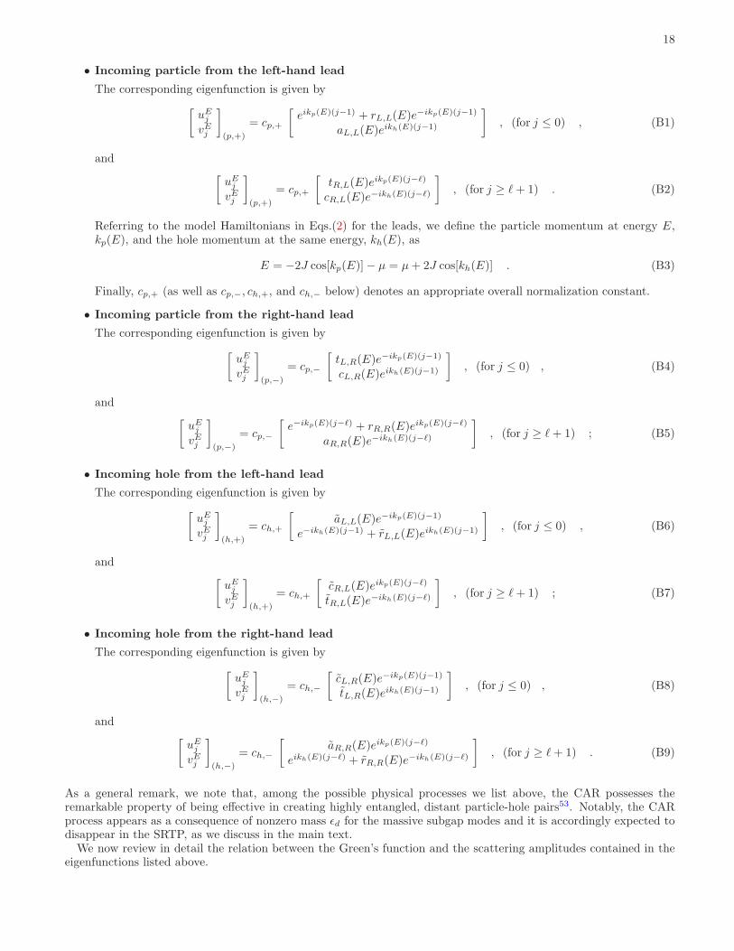
18

• Incoming particle from the left-hand lead

The corresponding eigenfunction is given by

[

uEj

vEj

]

(p,+)

= cp,+

[

eikp(E)(j−1) + rL,L(E)e−ikp(E)(j−1)

aL,L(E)eikh(E)(j−1)

]

, (for j ≤ 0) , (B1)

and[

uEj

vEj

]

(p,+)

= cp,+

[

tR,L(E)eikp(E)(j−ℓ)

cR,L(E)e−ikh(E)(j−ℓ)

]

, (for j ≥ ℓ+ 1) . (B2)

Referring to the model Hamiltonians in Eqs.(2) for the leads, we define the particle momentum at energy E,kp(E), and the hole momentum at the same energy, kh(E), as

E = −2J cos[kp(E)]− µ = µ+ 2J cos[kh(E)] . (B3)

Finally, cp,+ (as well as cp,−, ch,+, and ch,− below) denotes an appropriate overall normalization constant.

• Incoming particle from the right-hand lead

The corresponding eigenfunction is given by

[

uEj

vEj

]

(p,−)

= cp,−

[

tL,R(E)e−ikp(E)(j−1)

cL,R(E)eikh(E)(j−1)

]

, (for j ≤ 0) , (B4)

and[

uEj

vEj

]

(p,−)

= cp,−

[

e−ikp(E)(j−ℓ) + rR,R(E)eikp(E)(j−ℓ)

aR,R(E)e−ikh(E)(j−ℓ)

]

, (for j ≥ ℓ+ 1) ; (B5)

• Incoming hole from the left-hand lead

The corresponding eigenfunction is given by

[

uEj

vEj

]

(h,+)

= ch,+

[

aL,L(E)e−ikp(E)(j−1)

e−ikh(E)(j−1) + rL,L(E)eikh(E)(j−1)

]

, (for j ≤ 0) , (B6)

and[

uEj

vEj

]

(h,+)

= ch,+

[

cR,L(E)eikp(E)(j−ℓ)

tR,L(E)e−ikh(E)(j−ℓ)

]

, (for j ≥ ℓ+ 1) ; (B7)

• Incoming hole from the right-hand lead

The corresponding eigenfunction is given by

[

uEj

vEj

]

(h,−)

= ch,−

[

cL,R(E)e−ikp(E)(j−1)

tL,R(E)eikh(E)(j−1)

]

, (for j ≤ 0) , (B8)

and[

uEj

vEj

]

(h,−)

= ch,−

[

aR,R(E)eikp(E)(j−ℓ)

eikh(E)(j−ℓ) + rR,R(E)e−ikh(E)(j−ℓ)

]

, (for j ≥ ℓ+ 1) . (B9)

As a general remark, we note that, among the possible physical processes we list above, the CAR possesses theremarkable property of being effective in creating highly entangled, distant particle-hole pairs53. Notably, the CARprocess appears as a consequence of nonzero mass ǫd for the massive subgap modes and it is accordingly expected todisappear in the SRTP, as we discuss in the main text.We now review in detail the relation between the Green’s function and the scattering amplitudes contained in the

eigenfunctions listed above.

19

2. Relation between the scattering amplitudes and the fully dressed Green’s functions of the system

To spell out the relation between scattering amplitudes and Green’s functions, we start by considering the Green’sfunctions in Eq.(A1), which can be readily expressed in terms of the solutions of the BdG equations, by going throughthe representation of the fermion operators in real space in terms of the eigenmodes of the whole system Hamiltonian.This is determined by the equations

cj =∑

E>0

∑

a

[uEj ]aΓE,a + [vEj ]

∗aΓ

†E,a

c†j =∑

E>0

∑

a

[vEj ]aΓE,a + [uEj ]

∗aΓ

†E,a , (B10)

with a ∈ (p,+), (p,−), (h,+), (h,−) and ΓE,a,Γ†E,a being the corresponding energy eigenmodes satisfying the

anticommutator algebra

ΓE,a,Γ†E′,a′ = δE,E′δa,a′ . . (B11)

As a result, inserting Eqs.(B11) into Eqs.(A1) and moving to the mixed (real space-frequency) representation, oneobtains

C(X,X′);(j,j′)(iω) =∑

E>0

∑

a

1

iω − E

[

(uEj )a(u

Ej′)

∗a (uE

j )a(vEj′ )

∗a

(vj)Ea (u

Ej′)

∗a (vj)

Ea (v

Ej′ )

∗a

]

+∑

E>0

∑

a

1

iω + E

[

(vEj )∗a(v

Ej′ )a (vEj )∗a(u

Ej′)a

(uEj )

∗a(v

Ej′ )a (uE

j )∗a(u

Ej′)a

]

,

(B12)with, respectively, (X,X ′) = (L,L) for j, j′ ≤ 0, (X,X ′) = (L,R) for j ≤ 0, j′ ≥ ℓ + 1, (X,X ′) = (R,L) forj ≥ ℓ+ 1, j′ ≤ 0, and (X,X ′) = (R,R) for j, j′ ≥ ℓ+ 1.Now, to keep in touch with the results that we provide in Eqs.(A17,A18,A19,A20), we compute the Green’s functions

in terms of the solutions of the BdG equations by expanding the momenta kp(E), kh(E) around the Fermi momentumkF , defined by −2J cos(kF )− µ = 0, as

kp(E) = kF +E

v

kh(E) = kF −E

v, (B13)

with the Fermi velocity v = 2J sin(kF ), which also corresponds to setting ω = 0 in the function v(ω), so that wesubstitute v(±ω) with v(ω = 0) = 2iJ sin(kF ) = iv. Without entering the details of a straightforward, though tedious,calculation, one eventually obtains

C(L,L);(j,j′)(iω) =1

iv

[

eikF |j−j′|−ωv|j−j′| 0

0 e−ikF |j−j′|−ωv|j−j′|

]

,

+1

iv

[

rL,L(iω)e−ikF (j+j′−2)+ω

v(j+j′−2) aL,L(iω)e

−ikF (j−j′)+ωv(j+j′−2)

aL,L(iω)eikF (j−j′)+ω

v(j+j′−2) rL,L(iω)e

ikF (j+j′−2)+ωv(j+j′−2)

]

, (B14)

C(L,R);(j,j′)(iω) =1

iv

[

tL,R(iω)e−ikF (j−j′+ℓ−1)+ω

v(j−j′+ℓ−1) cL,R(iω)e

−ikF (j+j′−ℓ−1)+ωv(j−j′+ℓ−1)

cL,R(iω)eikF (j+j′−ℓ−1)+ω

v(j−j′+ℓ−1) tL,R(iω)e

ikF (j−j′+ℓ−1)+ωv(j−j′+ℓ−1)

]

, (B15)

C(R,L);(j,j′)(iω) =1

iv

[

tR,L(iω)eikF (j−j′−ℓ+1)−ω

v(j−j′−ℓ+1) cR,L(iω)e

ikF (j+j′−ℓ−1)−ωv(j−j′−ℓ+1)

cR,L(iω)e−ikF (j+j′−ℓ−1)−ω

v(j−j′−ℓ+1) tR,L(iω)e

−ikF (j−j′−ℓ+1)+ωv(j−j′−ℓ+1)

]

. (B16)

and, finally

C(R,R);(j,j′)(iω) =1

iv

[

eikF |j−j′|−ωv|j−j′| 0

0 e−ikF |j−j′|−ωv|j−j′|

]

+1

iv

[

rR,R(iω)eikF (j+j′−2ℓ)−ω

v(j+j′−2ℓ) aR,R(iω)e

ikF (j−j′)−ωv(j+j′−2ℓ)

aR,R(iω)e−ikF (j−j′)−ω

v(j+j′−2ℓ) rR,R(iω)e

−ikF (j+j′−2ℓ)−ωv(j+j′−2ℓ)

]

. (B17)

20

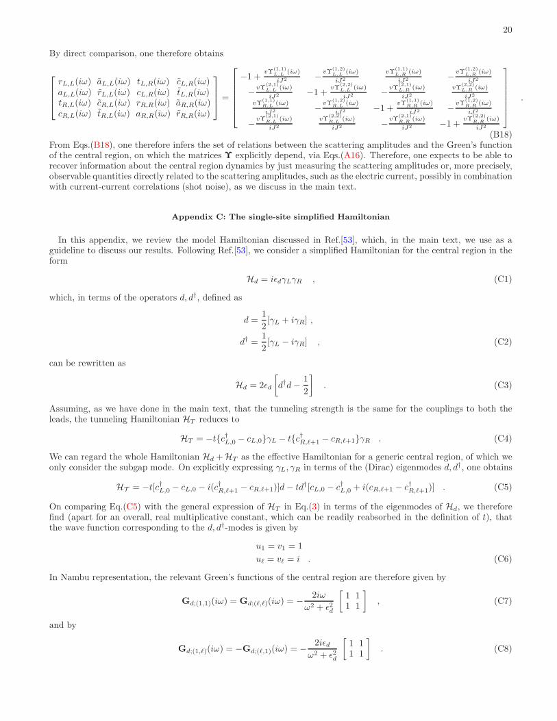
By direct comparison, one therefore obtains

rL,L(iω) aL,L(iω) tL,R(iω) cL,R(iω)aL,L(iω) rL,L(iω) cL,R(iω) tL,R(iω)tR,L(iω) cR,L(iω) rR,R(iω) aR,R(iω)cR,L(iω) tR,L(iω) aR,R(iω) rR,R(iω)

=

−1 +vΥ

(1,1)L,L

(iω)

iJ2 −vΥ

(1,2)L,L

(iω)

iJ2

vΥ(1,1)L,R

(iω)

iJ2 −vΥ

(1,2)L,R

(iω)

iJ2

−vΥ

(2,1)L,L

(iω)

iJ2 −1 +vΥ

(2,2)L,L

(iω)

iJ2 −vΥ

(2,1)L,R

(iω)

iJ2

vΥ(2,2)L,R

(iω)

iJ2

vΥ(1,1)R,L

(iω)

iJ2 −vΥ

(1,2)R,L

(iω)

iJ2 −1 +vΥ

(1,1)R,R

(iω)

iJ2 −vΥ

(1,2)R,R

(iω)

iJ2

−vΥ

(2,1)R,L

(iω)

iJ2

vΥ(2,2)R,L

(iω)

iJ2 −vΥ

(2,1)R,R

(iω)

iJ2 −1 +vΥ

(2,2)R,R

(iω)

iJ2

.

(B18)From Eqs.(B18), one therefore infers the set of relations between the scattering amplitudes and the Green’s functionof the central region, on which the matrices Υ explicitly depend, via Eqs.(A16). Therefore, one expects to be able torecover information about the central region dynamics by just measuring the scattering amplitudes or, more precisely,observable quantities directly related to the scattering amplitudes, such as the electric current, possibly in combinationwith current-current correlations (shot noise), as we discuss in the main text.

Appendix C: The single-site simplified Hamiltonian

In this appendix, we review the model Hamiltonian discussed in Ref.[53], which, in the main text, we use as aguideline to discuss our results. Following Ref.[53], we consider a simplified Hamiltonian for the central region in theform

Hd = iǫdγLγR , (C1)

which, in terms of the operators d, d†, defined as

d =1

2[γL + iγR] ,

d† =1

2[γL − iγR] , (C2)

can be rewritten as

Hd = 2ǫd

[

d†d−1

2

]

. (C3)

Assuming, as we have done in the main text, that the tunneling strength is the same for the couplings to both theleads, the tunneling Hamiltonian HT reduces to

HT = −tc†L,0 − cL,0γL − tc†R,ℓ+1 − cR,ℓ+1γR . (C4)

We can regard the whole Hamiltonian Hd +HT as the effective Hamiltonian for a generic central region, of which weonly consider the subgap mode. On explicitly expressing γL, γR in terms of the (Dirac) eigenmodes d, d†, one obtains

HT = −t[c†L,0 − cL,0 − i(c†R,ℓ+1 − cR,ℓ+1)]d− td†[cL,0 − c†L,0 + i(cR,ℓ+1 − c†R,ℓ+1)] . (C5)

On comparing Eq.(C5) with the general expression of HT in Eq.(3) in terms of the eigenmodes of Hd, we thereforefind (apart for an overall, real multiplicative constant, which can be readily reabsorbed in the definition of t), thatthe wave function corresponding to the d, d†-modes is given by

u1 = v1 = 1

uℓ = vℓ = i . (C6)

In Nambu representation, the relevant Green’s functions of the central region are therefore given by

Gd;(1,1)(iω) = Gd;(ℓ,ℓ)(iω) = −2iω

ω2 + ǫ2d

[

1 11 1

]

, (C7)

and by

Gd;(1,ℓ)(iω) = −Gd;(ℓ,1)(iω) = −2iǫd

ω2 + ǫ2d

[

1 11 1

]

. (C8)

21

In order to perform a comparison with the results of Ref.[53], we have to go through a further low-energy approxima-

tion, in neglecting the dependence on ω in C(0)(L,L);(0,0)(iω), which yields

Υ(L,L)(iω) =

[

1

(Jω − 4t2 sin(kF ))2 + J2ǫ2d

] [

−2it2(Jω − 4t2 sin(kF )) 2it2(Jω − 4t2 sin(kF ))2it2(Jω − 4t2 sin(kF )) −2it2(Jω − 4t2 sin(kF ))

]

, (C9)

Υ(L,R)(iω) =

[

1

(Jω − 4t2 sin(kF ))2 + J2ǫ2d

] [

−2iJt2ǫd 2iJt2ǫd2iJt2ǫd −2iJt2ǫd

]

, (C10)

Υ(R,L)(iω) =

[

1

(Jω − 4t2 sin(kF ))2 + J2ǫ2d

] [

2iJt2ǫd −2iJt2ǫd−2iJt2ǫd 2iJt2ǫd

]

, (C11)

and, finally

Υ(R,R)(iω) =

[

1

(Jω − 4t2 sin(kF ))2 + J2ǫ2d

] [

−2it2(Jω − 4t2 sin(kF )) 2it2(Jω − 4t2 sin(kF ))2it2(Jω − 4t2 sin(kF )) −2it2(Jω − 4t2 sin(kF ))

]

. (C12)

Accordingly, the scattering amplitudes are given by[

rL,L(iω) aL,L(iω)aL,L(iω) rL,L(iω)

]

=

[

rR,R(iω) aR,R(iω)aR,R(iω) rR,R(iω)

]

=

[

−1− α(iω) −α(iω)−α(iω) −1− α(iω)

]

, (C13)

with

α(iω) =4t2 sin(kF )(Jω − 4t2 sin(kF ))

(Jω − 4t2 sin(kF ))2 + J2ǫ2d, (C14)

and[

tL,R(iω) cL,R(iω)cL,R(iω) tL,R(iω)

]

= −

[

tR,L(iω) cR,L(iω)cR,L(iω) tR,L(iω)

]

=

[

−β(iω) −β(iω)−β(iω) −β(iω)

]

, (C15)

being

β(iω) =4t2 sin(kF )Jǫd

(Jω − 4t2 sin(kF ))2 + J2ǫ2d. (C16)

On back-rotating to real energies, we have to substitute iω with E + i0+, which implies

α(iω) → α(E) = −Γ(iE + Γ)

(iE + Γ)2 + ǫ2d

β(iω) → β(E) =Γǫd

(iE + Γ)2 + ǫ2d, (C17)

where we have set Γ = 4t2 sin(kF )/J . This is the basic result for the scattering amplitudes derived in Ref.[53], whichwe used as a reference model Hamiltonian to discuss the subgap physics of our system.

Appendix D: Derivation of the current and of the shot-noise in the NSN junction

In this appendix, we review and discuss the derivation of the transport properties of the NSN junction. To do so,we rely on the Landauer-like scattering approach, in which one imagines to ”shoot in” particles and holes againstthe SN interfaces from a thermal lead at temperature T : This allows us to recover the full expression of the currentand of the zero-frequency shot-noise just in terms of the single-particle and of the single hole scattering amplitudes.The approach we are going to review in the following is an adapted version of the general formalism developed anddiscussed in details in Ref.[65].Our starting point is the electric current operator over the link from j to j + 1, which takes the form

Jj = −ieJc†jcj+1 − c†j+1cj . (D1)

22

Once expanding the single-fermion operators in the basis of the eigenstates obeying the scattering boundary conditions,according to the Bogoliubov-Valatin transformations in Eqs.(B10), one obtains that the current operator in theHeisenberg representation takes the form

Jj(t) =∑

a,a′

∑

E,E′>0

J(a,a′);(E,E′)(+,−);j ei(E−E′)tΓ†

a,EΓa′,E′ + J(a,a′);(E,E′)(−,+);j e−i(E−E′)tΓa,EΓ

†a′,E′

+ J(a,a′);(E,E′)(+,+);j ei(E+E′)tΓ†

a,EΓ†a′,E′ + J

(a,a′);(E,E′)(−,−);j e−i(E+E′)tΓa,EΓa′,E′ , (D2)

with

J(a,a′);(E,E′)(+,−);j = −ieJ(uE

j )∗a(u

E′

j+1)a′ − (uEj+1)

∗a(u

E′

j )a′

J(a,a′);(E,E′)(−,+);j = −ieJ(vEj )a(v

E′

j+1)∗a′ − (vEj+1)a(v

E′

j )∗a′

J(a,a′);(E,E′)(+,+);j = −ieJ(uE

j )∗a(v

E′

j+1)∗a′ − (uE

j+1)∗a(v

E′

j )∗a′

J(a,a′);(E,E′)(−,−);j = −ieJ(vEj )a(u

E′

j+1)a′ − (vEj+1)a(uE′

j )a′ . (D3)

Using Eqs.(D2, D3), in the following we compute the current, as well as the zero-frequency shot noise.

1. Current flowing across the normal leads

Assuming that the two leads are biased at a voltage V with respect to the central region, basically means thatparticles and/or holes enter the central region from thermal reservoirs, so that particles emerge from the reservoirs ata chemical potential µ−eV , µ being the equilibrium chemical potential of the whole NSN junction, while, accordingly,holes emerge at a chemical potential µ+ eV . In terms of average energy of the eigenmodes of the total Hamiltonian,this basically implies

〈Γ†a,EΓa′,E′〉 = δa,a′δE,E′ f(E − eV ) if a ∈ (p,+), (p,−)

〈Γ†a,EΓa′,E′〉 = δa,a′δE,E′ f(E + eV ) if a ∈ (h,+), (h,−)

〈Γ†a,EΓ

†a′,E′〉 = 〈Γa,EΓa′,E′〉 = 0 , (D4)

with f(E) being the Fermi distribution function with chemical potential µ. Taking Eqs.(D4) into account andconsidering the explicit form of the current operator, one eventually obtains, in the zero-temperature limit

IL →2e

2π

∫ eV

0

dE |aL,L(E)|2 + |cL,R(E)|2 ,

IR → −2e

2π

∫ eV

0

dE |aR,R(E)|2 + |cR,L(E)|2 . (D5)

As a next step, we now compute the zero-frequency shot noise.

2. Zero-frequency shot noise

The zero-frequency shot noise at voltage bias V is defined from the Fourier transform of the real-time current-currentcorrelation functions. In general, considering current operators in sites j, j′, one sets

Rj,j′(Ω) =

∫ ∞

−∞

dt eiΩt 1

2〈δJj(t), δJj′ (0)〉 , (D6)

with

δJj(t) = Jj(t)− 〈Jj(t)〉 . (D7)

Therefore, the zero-frequency noise power is defined as

Pj,j′ = limΩ→0

Rj,j′ (Ω) . (D8)

23

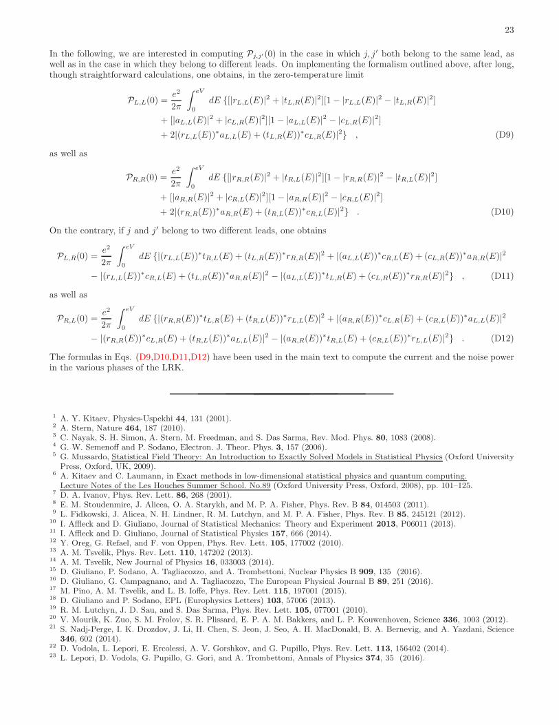
In the following, we are interested in computing Pj,j′(0) in the case in which j, j′ both belong to the same lead, aswell as in the case in which they belong to different leads. On implementing the formalism outlined above, after long,though straightforward calculations, one obtains, in the zero-temperature limit

PL,L(0) =e2

2π

∫ eV

0

dE [|rL,L(E)|2 + |tL,R(E)|2][1 − |rL,L(E)|2 − |tL,R(E)|2]

+ [|aL,L(E)|2 + |cL,R(E)|2][1 − |aL,L(E)|2 − |cL,R(E)|2]

+ 2|(rL,L(E))∗aL,L(E) + (tL,R(E))∗cL,R(E)|2 , (D9)

as well as

PR,R(0) =e2

2π

∫ eV

0

dE [|rR,R(E)|2 + |tR,L(E)|2][1− |rR,R(E)|2 − |tR,L(E)|2]

+ [|aR,R(E)|2 + |cR,L(E)|2][1− |aR,R(E)|2 − |cR,L(E)|2]

+ 2|(rR,R(E))∗aR,R(E) + (tR,L(E))∗cR,L(E)|2 . (D10)

On the contrary, if j and j′ belong to two different leads, one obtains

PL,R(0) =e2

2π

∫ eV

0

dE |(rL,L(E))∗tR,L(E) + (tL,R(E))∗rR,R(E)|2 + |(aL,L(E))∗cR,L(E) + (cL,R(E))∗aR,R(E)|2

− |(rL,L(E))∗cR,L(E) + (tL,R(E))∗aR,R(E)|2 − |(aL,L(E))∗tL,R(E) + (cL,R(E))∗rR,R(E)|2 , (D11)

as well as

PR,L(0) =e2

2π

∫ eV

0

dE |(rR,R(E))∗tL,R(E) + (tR,L(E))∗rL,L(E)|2 + |(aR,R(E))∗cL,R(E) + (cR,L(E))∗aL,L(E)|2

− |(rR,R(E))∗cL,R(E) + (tR,L(E))∗aL,L(E)|2 − |(aR,R(E))∗tR,L(E) + (cR,L(E))∗rL,L(E)|2 . (D12)

The formulas in Eqs. (D9,D10,D11,D12) have been used in the main text to compute the current and the noise powerin the various phases of the LRK.

1 A. Y. Kitaev, Physics-Uspekhi 44, 131 (2001).2 A. Stern, Nature 464, 187 (2010).3 C. Nayak, S. H. Simon, A. Stern, M. Freedman, and S. Das Sarma, Rev. Mod. Phys. 80, 1083 (2008).4 G. W. Semenoff and P. Sodano, Electron. J. Theor. Phys. 3, 157 (2006).5 G. Mussardo, Statistical Field Theory: An Introduction to Exactly Solved Models in Statistical Physics (Oxford UniversityPress, Oxford, UK, 2009).

6 A. Kitaev and C. Laumann, in Exact methods in low-dimensional statistical physics and quantum computing.Lecture Notes of the Les Houches Summer School. No.89 (Oxford University Press, Oxford, 2008), pp. 101–125.

7 D. A. Ivanov, Phys. Rev. Lett. 86, 268 (2001).8 E. M. Stoudenmire, J. Alicea, O. A. Starykh, and M. P. A. Fisher, Phys. Rev. B 84, 014503 (2011).9 L. Fidkowski, J. Alicea, N. H. Lindner, R. M. Lutchyn, and M. P. A. Fisher, Phys. Rev. B 85, 245121 (2012).

10 I. Affleck and D. Giuliano, Journal of Statistical Mechanics: Theory and Experiment 2013, P06011 (2013).11 I. Affleck and D. Giuliano, Journal of Statistical Physics 157, 666 (2014).12 Y. Oreg, G. Refael, and F. von Oppen, Phys. Rev. Lett. 105, 177002 (2010).13 A. M. Tsvelik, Phys. Rev. Lett. 110, 147202 (2013).14 A. M. Tsvelik, New Journal of Physics 16, 033003 (2014).15 D. Giuliano, P. Sodano, A. Tagliacozzo, and A. Trombettoni, Nuclear Physics B 909, 135 (2016).16 D. Giuliano, G. Campagnano, and A. Tagliacozzo, The European Physical Journal B 89, 251 (2016).17 M. Pino, A. M. Tsvelik, and L. B. Ioffe, Phys. Rev. Lett. 115, 197001 (2015).18 D. Giuliano and P. Sodano, EPL (Europhysics Letters) 103, 57006 (2013).19 R. M. Lutchyn, J. D. Sau, and S. Das Sarma, Phys. Rev. Lett. 105, 077001 (2010).20 V. Mourik, K. Zuo, S. M. Frolov, S. R. Plissard, E. P. A. M. Bakkers, and L. P. Kouwenhoven, Science 336, 1003 (2012).21 S. Nadj-Perge, I. K. Drozdov, J. Li, H. Chen, S. Jeon, J. Seo, A. H. MacDonald, B. A. Bernevig, and A. Yazdani, Science

346, 602 (2014).22 D. Vodola, L. Lepori, E. Ercolessi, A. V. Gorshkov, and G. Pupillo, Phys. Rev. Lett. 113, 156402 (2014).23 L. Lepori, D. Vodola, G. Pupillo, G. Gori, and A. Trombettoni, Annals of Physics 374, 35 (2016).

24

24 D. Vodola, L. Lepori, E. Ercolessi, and G. Pupillo, New Journal of Physics 18, 015001 (2016).25 O. Viyuela, D. Vodola, G. Pupillo, and M. A. Martin-Delgado, Phys. Rev. B 94, 125121 (2016).26 P. Hauke and L. Tagliacozzo, Phys. Rev. Lett. 111, 207202 (2013).27 L. Lepori and L. Dell’Anna, New Journal of Physics 19, 103030 (2017).28 O. Viyuela, L. Fu, and M. A. Martin-Delgado, Phys. Rev. Lett. 120, 017001 (2018).29 L. Lepori, D. Giuliano, and S. Paganelli, Phys. Rev. B 97, 041109(R) (2018).30 M. Burrello, I. C. Fulga, E. Alba, L. Lepori, and A. Trombettoni, Phys. Rev. A 88, 053619 (2013).31 M. Benito, A. Gomez-Leon, V. M. Bastidas, T. Brandes, and G. Platero, Phys. Rev. B 90, 205127 (2014).32 Z.-Z. Li, C.-H. Lam, and J. Q. You, Phys. Rev. B 96, 155438 (2017).33 P. Nevado, S. Fernandez-Lorenzo, and D. Porras, Phys. Rev. Lett. 119, 210401 (2017).34 P. Richerme, Z.-X. Gong, A. Lee, C. Senko, J. Smith, M. Foss Feigh, S. Michalakis, A. V. Gorshkov, and C. Monroe, Nature

(London) 511, 198 (2014).35 P. Jurcevic, B. P. Lanyon, P. Hauke, C. Hempel, P. Zoller, R. Blatt, and C. F. Roos, Nature (London) 511, 202 (2014).36 C. Schneider, D. Porras, and T. Schaetz, Reports on Progress in Physics 75, 024401 (2012).37 S. Gopalakrishnan, B. L. Lev, and P. M. Goldbart, Phys. Rev. Lett. 107, 277201 (2011).38 E. Shahmoon and G. Kurizki, Phys. Rev. A 87, 033831 (2013).39 J. Perczel, J. Borregaard, D. E. Chang, H. Pichler, S. F. Yelin, P. Zoller, and M. D. Lukin, Phys. Rev. Lett. 119, 023603

(2017).40 R. J. Bettles, J. c. v. Minar, C. S. Adams, I. Lesanovsky, and B. Olmos, Phys. Rev. A 96, 041603 (2017).41 F. Pientka, L. I. Glazman, and F. von Oppen, Phys. Rev. B 89, 180505 (2014).42 F. Pientka, L. I. Glazman, and F. von Oppen, Phys. Rev. B 88, 155420 (2013).43 J. P. Blaizot and G. Ripka, Quantum Theory of Finite Systems (The MIT Press, Cambridge, Massachusetts, 1986).44 A. Altland and M. R. Zirnbauer, Phys. Rev. B 55, 1142 (1997).45 A. P. Schnyder, S. Ryu, A. Furusaki, and A. W. W. Ludwig, Phys. Rev. B 78, 195125 (2008).46 A. P. Schnyder, S. Ryu, A. Furusaki, and A. W. W. Ludwig, AIP Conference Proceedings 1134, 10 (2009).47 K. Patrick, T. Neupert, and J. K. Pachos, Phys. Rev. Lett. 118, 267002 (2017).48 J. Eisert, M. Cramer, and M. B. Plenio, Rev. Mod. Phys. 82, 277 (2010).49 F. Ares, J. G. Esteve, F. Falceto, and A. R. de Queiroz, Phys. Rev. A 92, 042334 (2015).50 S. Sachdev, Quantum phase transitions (second edition) (Cambridge University Press, Cambridge, UK, 2011).51 P. Zanardi, P. Giorda, and M. Cozzini, Phys. Rev. Lett. 99, 100603 (2007).52 L. Pezze, M. Gabbrielli, L. Lepori, and A. Smerzi, Phys. Rev. Lett. 119, 250401 (2017).53 J. Nilsson, A. R. Akhmerov, and C. W. J. Beenakker, Phys. Rev. Lett. 101, 120403 (2008).54 M. Tinkham, Introduction to Superconductivity: Second Edition (Dover Publications, Oxford, UK, 2004).55 A. Nava, R. Giuliano, G. Campagnano, and D. Giuliano, Phys. Rev. B 94, 205125 (2016).56 C. J. Bolech and E. Demler, Phys. Rev. Lett. 98, 237002 (2007).57 K. T. Law, P. A. Lee, and T. K. Ng, Phys. Rev. Lett. 103, 237001 (2009).58 A. Golub and B. Horovitz, Phys. Rev. B 83, 153415 (2011).59 Y. Cao, P. Wang, G. Xiong, M. Gong, and X.-Q. Li, Phys. Rev. B 86, 115311 (2012).60 Y. V. Nazarov and Y. M. Blanter, Quantum Transport: Introduction to Nanoscience (Cambridge University Press, 2009).61 G. E. Blonder, M. Tinkham, and T. M. Klapwijk, Phys. Rev. B 25, 4515 (1982).62 M. Octavio, M. Tinkham, G. E. Blonder, and T. M. Klapwijk, Phys. Rev. B 27, 6739 (1983).63 N. N. Bogoli’Ubov and D. V. Shirkov, Introduction to the theory of quantized fields (1959).64 G. D. Mahan, Many-Particle Physics (Plenum Press, New York, NY, 1990).65 M. P. Anantram and S. Datta, Phys. Rev. B 53, 16390 (1996).