1 indexing and hashing indexing and hashing basic concepts dense and sparse indices b+trees, b-trees...

1

Indexing and HashingIndexing and Hashing

Basic Concepts

Dense and Sparse Indices

B+Trees, B-trees

Dynamic Hashing

Comparison of Ordered Indexing and Hashing

Index Definition in SQL

Multiple-Key Access

2

Basic ConceptsBasic Concepts Indexing mechanisms used to speed up access to desired data.

E.g., author catalog in library

Search Key - attribute to set of attributes used to look up records in a file.

An index file consists of records (called index entries) of the form

Index files are typically much smaller than the original file

Two basic kinds of indices:

Ordered indices: search keys are stored in sorted order

Hash indices: search keys are distributed uniformly across “buckets” using a “hash function”.

search-key pointer

3

Index Evaluation MetricsIndex Evaluation Metrics

Access types supported efficiently. E.g.,

records with a specified value in the attribute

or records with an attribute value falling in a specified range of values.

Access time

Insertion time

Deletion time

Space overhead

4

Ordered IndicesOrdered Indices

In an ordered index, index entries are stored sorted on the search key value. E.g., author catalog in library.

Primary index: in a sequentially ordered file, the index whose search key specifies the sequential order of the file.

Also called clustering index

The search key of a primary index is usually but not necessarily the primary key.

Secondary index: an index whose search key specifies an order different from the sequential order of the file. Also called non-clustering index.

Index-sequential file: ordered sequential file with a primary index.

5

Sequential File

2010

4030

6050

8070

10090

6

Sequential File

2010

4030

6050

8070

10090

Dense Index

10203040

50607080

90100110120

7

Sequential File

2010

4030

6050

8070

10090

Sparse Index

10305070

90110130150

170190210230

8

Sequential File

2010

4030

6050

8070

10090

Sparse 2nd level

10305070

90110130150

170190210230

1090

170250

330410490570

9

Sparse vs. Dense TradeoffSparse vs. Dense Tradeoff

Sparse:

Less index space per record can keep more of index in memory

Dense:

Can tell if any record exists without accessing file

10

Dense and Sparse Index Update OperationsDense and Sparse Index Update Operations

Duplicate keys

Deletion/Insertion

Secondary indexes

11

Duplicate keysDuplicate keys

1010

2010

3020

3030

4540

12

1010

2010

3020

3030

4540

10101020

20303030

1010

2010

3020

3030

4540

10101020

20303030

Dense index, one way to implement?Dense index, one way to implement?


13

1010

2010

3020

3030

4540

10203040

Dense index, better way?Dense index, better way?


14

1010

2010

3020

3030

4540

10102030

Sparse index, one way?Sparse index, one way?

Duplicate keysDuplicate keysca

refu

l if lookin

gfo

r 2

0 o

r 3

0!

15

1010

2010

3020

3030

4540

10203040

Sparse index, another way?Sparse index, another way?


– place first new key from block

16

Duplicate values, Duplicate values, primary index primary index

Index may point to first instance of each value only

Index File

Summary

aaa

b

17

Deletion from sparse indexDeletion from sparse index

2010

4030

6050

8070

10305070

90110130150

18


2010

4030

6050

8070

10305070

90110130150

– delete record 40

19


2010

4030

6050

8070

10405070

90110130150


40

20


2010

4030

6050

8070

10305070

90110130150

– delete records 30 & 40

5070

21

Deletion from dense indexDeletion from dense index

2010

4030

6050

8070

10203040

50607080


4040

22

Insertion, sparse index caseInsertion, sparse index case

2010

30

5040

60

10304060

23


2010

30

5040

60

10304060

– insert record 34

34

24


2010

30

5040

60

10304060


15

2030

20

• Illustrated: Immediate reorganization• Variation:

– insert new block (chained file)– update index

25


2010

30

5040

60

10304060


25

overflow blocks(reorganize later...)

26

Sparse vs Dense IndicesSparse vs Dense Indices

Sparse Less index space per record

Can keep more of index in memory

Better for insertions

Dense Finds whether the record exists without file accessing

Required for secondary indices

27

Conventional indexesConventional indexes

Advantage:

- Simple- Index is sequential file

good for scans

Disadvantage:- Inserts expensive, and/or- Lose sequentiality & balance

28

BB++-Tree Index Files-Tree Index Files

Disadvantage of indexed-sequential files: performance degrades as file grows, since many overflow blocks get created. Periodic reorganization of entire file is required.

Advantage of B+-tree index files: automatically reorganizes itself with small, local, changes, in the face of insertions and deletions. Reorganization of entire file is not required to maintain performance.

Disadvantage of B+-trees: extra insertion and deletion overhead, space overhead.

Advantages of B+-trees outweigh disadvantages, and they are used extensively.

B+-tree indices are an alternative to indexed-sequential files.

29

BB++-Tree Index Files (Cont.)-Tree Index Files (Cont.)

All paths from root to leaf are of the same length

Each node that is not a root or a leaf has between [n/2] and n children.

A leaf node has between [(n–1)/2] and n–1 values

Special cases: If the root is not a leaf, it has at least 2 children.

If the root is a leaf (that is, there are no other nodes in the tree), it can have between 0 and (n–1) values.

A B+-tree is a rooted tree satisfying the following properties:

30

BB++-Tree Node Structure-Tree Node Structure

Typical node

Ki are the search-key values

Pi are pointers to children (for non-leaf nodes) or pointers to records or buckets of records (for leaf nodes).

The search-keys in a node are ordered

K1 < K2 < K3 < . . . < Kn–1

31

Leaf Nodes in BLeaf Nodes in B++-Trees-Trees

For i = 1, 2, . . ., n–1, pointer Pi either points to a file record with search-key value Ki, or to a bucket of pointers to file records, each record having search-key value Ki. Only need bucket structure if search-key does not form a primary key.

If Li, Lj are leaf nodes and i < j, Li’s search-key values are less than Lj’s search-key values

Pn points to next leaf node in search-key order

Properties of a leaf node:

32

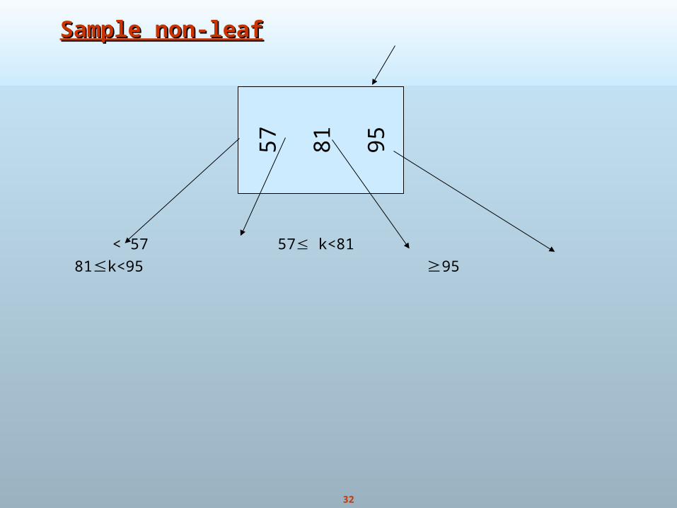
Sample non-leafSample non-leaf

< 57 57 k<81 81k<95 95

57

81

95

33

Example of a BExample of a B++-tree-tree

B+-tree for account file (n = 3)

34

Example of BExample of B++-tree-tree

Leaf nodes must have between 2 and 4 key values ((n–1)/2 and n –1, with n = 5).

Non-leaf nodes other than root must have between 3 and 5 children ((n/2 and n with n =5).

Root must have at least 2 children.

B+-tree for account file (n = 5)

35

Observations about BObservations about B++-trees-trees

Since the inter-node connections are done by pointers, “logically” close blocks need not be “physically” close.

The non-leaf levels of the B+-tree form a hierarchy of sparse indices.

The B+-tree contains a relatively small number of levels (logarithmic in the size of the main file), thus searches can be conducted efficiently.

Insertions and deletions to the main file can be handled efficiently, as the index can be restructured in logarithmic time (as we shall see).

36

Queries on BQueries on B++-Trees-Trees

Find all records with a search-key value of k.

1. Start with the root node

1. Examine the node for the smallest search-key value > k.

2. If such a value exists, assume it is Kj. Then follow Pi to the child node

3. Otherwise k Km–1, where there are m pointers in the node. Then follow Pm to the child node.

2. If the node reached by following the pointer above is not a leaf node, repeat the above procedure on the node, and follow the corresponding pointer.

3. Eventually reach a leaf node. If for some i, key Ki = k follow pointer Pi to the desired record or bucket. Else no record with search-key value k exists.

37

Queries on BQueries on B+-+-Trees (Cont.)Trees (Cont.)

In processing a query, a path is traversed in the tree from the root to some leaf node.

If there are K search-key values in the file, the path is no longer than logn/2(K).

A node is generally the same size as a disk block, typically 4 kilobytes, and n is typically around 100 (40 bytes per index entry).

With 1 million search key values and n = 100, at most log50(1,000,000) = 4 nodes are accessed in a lookup.

Contrast this with a balanced binary free with 1 million search key values — around 20 nodes are accessed in a lookup above difference is significant since every node access

may need a disk I/O, costing around 20 milliseconds!

38

Updates on BUpdates on B++-Trees: Insertion-Trees: Insertion

Find the leaf node in which the search-key value would appear

If the search-key value is already there in the leaf node, record is added to file and if necessary a pointer is inserted into the bucket.

If the search-key value is not there, then add the record to the main file and create a bucket if necessary. Then: If there is room in the leaf node, insert (key-value, pointer) pair in the

leaf node

Otherwise, split the node (along with the new (key-value, pointer) entry) as discussed in the next slide.

39

Updates on BUpdates on B++-Trees: Insertion (Cont.)-Trees: Insertion (Cont.)

Splitting a node: take the n(search-key value, pointer) pairs (including the one being

inserted) in sorted order. Place the first n/2 in the original node, and the rest in a new node.

let the new node be p, and let k be the least key value in p. Insert (k,p) in the parent of the node being split. If the parent is full, split it and propagate the split further up.

The splitting of nodes proceeds upwards till a node that is not full is found. In the worst case the root node may be split increasing the height of the tree by 1.

Result of splitting node containing Brighton and Downtown on inserting Clearview

40

Updates on BUpdates on B++-Trees: Insertion (Cont.)-Trees: Insertion (Cont.)

B+-Tree before and after insertion of “Clearview”

41

Updates on BUpdates on B++-Trees: Deletion-Trees: Deletion

Find the record to be deleted, and remove it from the main file and from the bucket (if present)

Remove (search-key value, pointer) from the leaf node if there is no bucket or if the bucket has become empty

If the node has too few entries due to the removal, and the entries in the node and a sibling fit into a single node, then Insert all the search-key values in the two nodes into a

single node (the one on the left), and delete the other node.

Delete the pair (Ki–1, Pi), where Pi is the pointer to the deleted node, from its parent, recursively using the above procedure.

42

Examples of BExamples of B++-Tree Deletion-Tree Deletion

The removal of the leaf node containing “Downtown” did not result in its parent having too little pointers. So the cascaded deletions stopped with the deleted leaf node’s parent.

Before and after deleting “Downtown”

43

Examples of BExamples of B++-Tree Deletion (Cont.)-Tree Deletion (Cont.)

Node with “Perryridge” becomes underfull (actually empty, in this special case) and merged with its sibling.

As a result “Perryridge” node’s parent became underfull, and was merged with its sibling (and an entry was deleted from their parent)

Root node then had only one child, and was deleted and its child became the new root node

Deletion of “Perryridge” from result of previous example

44

Example of BExample of B++-tree Deletion (Cont.)-tree Deletion (Cont.)

Parent of leaf containing Perryridge became underfull, and borrowed a pointer from its left sibling

Search-key value in the parent’s parent changes as a result

Before and after deletion of “Perryridge” from earlier example

45

B-Tree Index FilesB-Tree Index Files

Similar to B+-tree, but B-tree allows search-key values to appear only once; eliminates redundant storage of search keys.

Search keys in nonleaf nodes appear nowhere else in the B-tree; an additional pointer field for each search key in a nonleaf node must be included.

Generalized B-tree leaf node

Nonleaf node – pointers Bi are the bucket or file record pointers.

46

B-Tree Index File ExampleB-Tree Index File Example

B-tree (above) and B+-tree (below) on same data

47

B-Tree Index Files (Cont.)B-Tree Index Files (Cont.)

Advantages of B-Tree indices: May use less tree nodes than a corresponding B+-Tree.

Sometimes possible to find search-key value before reaching leaf node.

Disadvantages of B-Tree indices: Only small fraction of all search-key values are found early

Non-leaf nodes are larger, so fan-out is reduced. Thus, B-Trees typically have greater depth than corresponding B+-Tree

Insertion and deletion more complicated than in B+-Trees

Implementation is harder than B+-Trees.

Typically, advantages of B-Trees do not out weigh disadvantages.

48

key h(key)

Hashing

<key>

.

.

Buckets(typically 1disk block)

49

.

.

.

Two alternatives

records

.

.

.

(1) key h(key)

50

(2) key h(key)

Index

recordkey 1

Two alternatives

Alt (2) for “secondary” search key

51

Example hash functionExample hash function

Key = ‘x1 x2 … xn’ n byte character string

Have b buckets h: add x1 + x2 + ….. xn

compute sum modulo b

52

This may not be best function …

Read Knuth Vol. 3 if you really need to select a good function.

Good hash Expected number of

function: keys/bucket is the

same for all buckets

53

Within a bucket:Within a bucket:

Do we keep keys sorted?

Yes, if CPU time critical

& Inserts/Deletes not too frequent

54

Next:Next: example to illustrate example to illustrateinserts, overflows, deletesinserts, overflows, deletes

h(K)

55

EXAMPLEEXAMPLE 2 records/bucket 2 records/bucket

INSERT:

h(a) = 1

h(b) = 2

h(c) = 1

h(d) = 0

0

1

2

3

d

ac

b

h(e) = 1

e

56

0

1

2

3

a

bc

e

d

EXAMPLE:EXAMPLE: deletion deletion

Delete:ef

fg

maybe move“g” up

cd

57

Rule of thumb:Rule of thumb: Try to keep space utilization

between 50% and 80%

Utilization = # keys used total # keys that fit

If < 50%, wasting space

If > 80%, overflows significantdepends on how good hash function is & on # keys/bucket

58

How do we cope with growth?How do we cope with growth?

Overflows and reorganizations

Dynamic hashing

Extensible

Linear

59

Dynamic HashingDynamic Hashing

Good for database that grows and shrinks in size Allows the hash function to be modified dynamically Extendable hashing – one form of dynamic hashing

Hash function generates values over a large range — typically b-bit integers, with b = 32.

At any time use only a prefix of the hash function to index into a table of bucket addresses.

Let the length of the prefix be i bits, 0 i 32.

Bucket address table size = 2i. Initially i = 0

Value of i grows and shrinks as the size of the database grows and shrinks.

Multiple entries in the bucket address table may point to a bucket.

Thus, actual number of buckets is < 2i

The number of buckets also changes dynamically due to coalescing and splitting of buckets.

60

General Extendable Hash Structure General Extendable Hash Structure

In this structure, i2 = i3 = i, whereas i1 = i – 1 (see next slide for details)

61

Use of Extendable Hash StructureUse of Extendable Hash Structure

Each bucket j stores a value ij; all the entries that point to the same bucket have the same values on the first ij bits.

To locate the bucket containing search-key Kj:

1. Compute h(Kj) = X

2. Use the first i high order bits of X as a displacement into bucket address table, and follow the pointer to appropriate bucket

To insert a record with search-key value Kj

follow same procedure as look-up and locate the bucket, say j.

If there is room in the bucket j insert record in the bucket.

Else the bucket must be split and insertion re-attempted (next slide.)

Overflow buckets used instead in some cases (will see shortly)

62

Updates in Extendable Hash Structure Updates in Extendable Hash Structure

If i > ij (more than one pointer to bucket j)

allocate a new bucket z, and set ij and iz to the old ij -+ 1.

make the second half of the bucket address table entries pointing to j to point to z

remove and reinsert each record in bucket j.

recompute new bucket for Kj and insert record in the bucket (further splitting is required if the bucket is still full)

If i = ij (only one pointer to bucket j)

increment i and double the size of the bucket address table.

replace each entry in the table by two entries that point to the same bucket.

recompute new bucket address table entry for Kj

Now i > ij so use the first case above.

To split a bucket j when inserting record with search-key value Kj:

63

Updates in Extendable Hash Structure Updates in Extendable Hash Structure (Cont.)(Cont.)

When inserting a value, if the bucket is full after several splits (that is, i reaches some limit b) create an overflow bucket instead of splitting bucket entry table further.

To delete a key value, locate it in its bucket and remove it. The bucket itself can be removed if it becomes empty (with

appropriate updates to the bucket address table). Coalescing of buckets can be done (can coalesce only with a

“buddy” bucket having same value of ij and same ij –1 prefix, if it is present)

Decreasing bucket address table size is also possible Note: decreasing bucket address table size is an expensive

operation and should be done only if number of buckets becomes much smaller than the size of the table

64

Linear HashingLinear Hashing

Linear Hashing (Litwin 1980)

C – key space

N – initial number of buckets

Each bucket can keep M keys

P – pointer to keep track of the bucket that needs to be split if an overflow occurs. Initially P=0.

H0 (c) = c(modN)

Hi (c) = c(mod2^i *N)

For any key c, either Hi(c) = H(i-1) (c) or

Hi(c) = H(i-1) (c)+2^(i-1) * N

65

Linear HashingLinear Hashing

…….

H(i+1) H(i+1) Hi Hi H(i+1) H(i+1)

p

66

Extendable Hashing vs. Other SchemesExtendable Hashing vs. Other Schemes

Benefits of extensible hashing: Hash performance does not degrade with growth of file

Minimal space overhead

Disadvantages of extensible hashing Extra level of indirection to find desired record

Bucket address table may itself become very big (larger than memory)

Need a tree structure to locate desired record in the structure!

Changing size of bucket address table is an expensive operation

Linear hashing is an alternative mechanism which avoids these disadvantages at the possible cost of more bucket overflows

67

Comparison of Ordered Indexing and HashingComparison of Ordered Indexing and Hashing

Cost of periodic re-organization

Relative frequency of insertions and deletions

Is it desirable to optimize average access time at the expense of worst-case access time?

Expected type of queries: Hashing is generally better at retrieving records having a specified

value of the key.

If range queries are common, ordered indices are to be preferred

1 indexing and hashing indexing and hashing basic concepts dense and sparse indices b+trees, b-trees...

Documents