1

Improved Adaptive Rejection Metropolis

Sampling AlgorithmsLuca Martino†, Jesse Read†, David Luengo‡

†Department of Signal Theory and Communications, Universidad Carlos III de Madrid.

Avenida de la Universidad 30, 28911 Leganes, Madrid, Spain.‡Department of Circuits and Systems Engineering, Universidad Politecnica de Madrid.

Carretera de Valencia Km. 7, 28031 Madrid, Spain.

E-mail: luca@tsc.uc3m.es, jread@tsc.uc3m.es, david.luengo@upm.es

Abstract

Markov Chain Monte Carlo (MCMC) methods, such as the Metropolis-Hastings (MH) algorithm,

are widely used for Bayesian inference. One of the most important challenges for any MCMC method

is speeding up the convergence of the Markov chain, which depends crucially on a suitable choice of

the proposal density. Adaptive Rejection Metropolis Sampling (ARMS) is a well-known MH scheme

that generates samples from one-dimensional target densities making use of adaptive piecewise linear

proposals constructed using support points taken from rejected samples. In this work we pinpoint a

crucial drawback of the adaptive procedure used in ARMS: support points might never be added inside

regions where the proposal is below the target. When this happens in many regions it leads to a poor

performance of ARMS, and the sequence of proposals never converges to the target. In order to overcome

this limitation, we propose two alternative adaptive schemes that guarantee convergence to the target

distribution. These two new schemes improve the adaptive strategy of ARMS, thus allowing us to simplify

the construction of the sequence of proposals. Numerical results show that the new algorithms outperform

the standard ARMS and other techniques.

Index Terms

Markov Chain Monte Carlo (MCMC) methods; Metropolis-Hastings (MH) algorithm; Adaptive

Rejection Metropolis Sampling (ARMS).

I. INTRODUCTION

Bayesian inference techniques and their implementation by means of sophisticated Monte Carlo (MC)

statistical methods, such as Markov chain Monte Carlo (MCMC) and sequential Monte Carlo (SMC)

arX

iv:1

205.

5494

v4 [

stat

.CO

] 8

Oct

201

2

2

approaches (also known as particle filters), has become a very active area of research over the last years

[Gilks et al., 1995a, Gamerman, 1997, Liu, 2004, Robert and Casella, 2004, Liang et al., 2010]. Monte

Carlo techniques are very powerful tools for numerical inference, stochastic optimization and simulation

of complex systems [Devroye, 1986, Fearnhead, 1998, Doucet et al., 2001, Jaeckel, 2002, Robert and

Casella, 2004].

Rejection sampling (RS) [Devroye, 1986, von Neumann, 1951] and the Metropolis-Hastings (MH)

algorithm are two well-known classical Monte Carlo methods for universal sampling [Metropolis and

Ulam, 1949, Metropolis et al., 1953, Hastings, 1970, Liu, 2004]. Indeed, they can be used to generate

samples (independent with the RS and correlated with MH) from virtually any target probability density

function (pdf) by drawing from a simpler proposal pdf. Consequently, these two methods have been

widely diffused and applied. Unfortunately, in some situations they present certain important limitations

and drawbacks as we describe below.

In the RS technique the generated samples are either accepted or rejected by an adequate test of the

ratio of the target, p(x), and the proposal density, π(x), with x ∈ D ⊆ R.1 An important limitation of

RS is the need to analytically establish an upper bound M for the ratio of these two pdfs, M ≥ p(x)π(x)

or equivalently Mπ(x) ≥ p(x), which is not always an easy task. Moreover, even using the best bound,

i.e. M = supx p(x)/π(x), the acceptance rate can be very low if the proposal is not similar to the target

pdf. On the oher hand, in the MH algorithm, depending on the choice of the proposal pdf, the correlation

among the samples in the Markov chain can be very high [Liu, 2004, Liang et al., 2010, Martino and

Mıguez, 2010]. Correlated samples provide less statistical information and the resulting chain can remain

trapped almost indefinitely in a local mode, meaning that convergence will be very slow in practice.

Moreover, determining how long the chain needs to be run in order to converge is a difficult task, leading

to the common practice of establishing a large enough burn-in period to ensure the chain’s convergence

[Gilks et al., 1995a, Gamerman, 1997, Liu, 2004, Liang et al., 2010].

In order to overcome these limitations several extensions of both techniques have been introduced

[Devroye, 1986, Liu, 2004, Liang et al., 2010], as well as methods combining them [Tierney, 1991,

1994]. Furthermore, in the literature there is great interest in adaptive MCMC approaches that can speed

up the convergence of the Markov chain [Haario et al., 2001, Gasemyr, 2003, Andrieu and Moulines,

2006, Andrieu and Thoms, 2008, Holden et al., 2009, Griffin and Walker, 2011]. Here we focus on two

1Note that we assume, as is commonly done in the literature, that both pdfs are known up to a normalization constant, and

we denote as po(x) ∝ p(x) and π(x) ∝ π(x) the normalized target and proposal pdfs.

3

of the most popular adaptive extensions, pointing out their important limitations, and proposing a novel

adaptive technique that can overcome them and leads to a much more efficient approach for drawing

samples from the target pdf.

One widely known extension of RS is the class of adaptive rejection sampling (ARS) methods [Gilks,

1992, Gilks and Wild, 1992, Gilks et al., 1997], which is an improvement of the standard RS technique

that ensures high acceptance rates with a moderate and bounded computational cost. Indeed, the standard

ARS algorithm of [Gilks and Wild, 1992] yields a sequence of proposal functions, {πt(x)}t∈N, that

converge towards the target pdf when the procedure is iterated. The basic mechanism of ARS is the

following. Given a set of support points, St = {s1, ..., smt}, ARS builds a proposal pdf composed of

truncated exponential pdfs inside the intervals (sj , sj+1] (0 ≤ j ≤ mt), considering also the open intervals

(−∞, s1] (corresponding to j = 0) and [smt,+∞) (associated to j = mt) when D = R. Then, when a

newly proposed sample x′, drawn from πt(x), is rejected, it is always added to the set of support points,

St+1 = St ∪ {x′}, which are used to build a refined proposal pdf, πt+1(x), for the next iteration.

Note that the proposal density used in ARS becomes quickly closer to the target pdf and the proportion

of accepted samples grows. Consequently, since the proposal pdf is only updated when a sample is rejected

and the probability of discarding a sample decreases quickly to zero, the computational cost is bounded

and remains moderate, i.e. the computational cost does not diverge due to this smart adaptive strategy

that improves the proposal pdf only when and where it is needed. Unfortunately, this algorithm can only

be used with log-concave target densities and hence also unimodal. Therefore, several generalizations

have been proposed [Gilks et al., 1995b, Hormann, 1995, Evans and Swartz, 1998, Gorur and Teh, 2011,

Martino and Mıguez, 2011] handling specific classes of target distributions or using jointly a MCMC

approach.

Indeed, for instance, another popular technique that combines the ARS and MH approaches in an

attempt to overcome the limitations of both methodologies is the Adaptive Rejection Metropolis Sampling

(ARMS) [Gilks et al., 1995b]. ARMS extends ARS to tackle multimodal and non-log-concave densities

by allowing the proposal to remain below the target in some regions and adding a Metropolis-Hastings

(MH) step to the algorithm to ensure that the accepted samples are properly distributed according to

the target pdf. Note that introducing the MH step means that, unlike in the original ARS method, the

resulting samples are correlated. The ARMS technique uses first an RS test on each generated sample

x′ and, if this sample is initially accepted, applies also an MH step to determine whether it is finally

accepted or not. If a sample x′ is rejected in the RS test (hence, imperatively πt(x′) ≥ p(x′), as otherwise

samples are always initially accepted by the RS step), then it is incorporated to the set of support points,

4

St+1 = St ∪{x′}, that is used to build a better proposal pdf for the next iteration, πt+1(x), exactly as in

ARS. On the other hand, when a sample is initially accepted, after the MH step the set of support points

is never updated, i.e. St+1 = St, meaning that the proposal pdf is not improved and πt+1(x) = πt(x).

This is the crucial point w.r.t. the performance of ARMS. In general, if proper procedures for

constructing πt(x) given a set of support points, St, such as the ones proposed in [Gilks et al., 1995b,

Meyer et al., 2008] are adopted, the proposal will improve throughout the whole domain x ∈ D. However,

inside the regions of the domain D where πt(x) < p(x), new support points might never be added.

Consequently, the convergence of the sequence {πt(x)}t∈N to p(x) cannot be guaranteed, and it may not

occur in some cases, as shown in Section IV through a simple example. Due to this problem and the

correlation among the samples generated, when the target pdf is multimodal the Markov chain generated

by the ARMS algorithm tends to get trapped in a single mode despite the (partial) adaptation of the

proposal pdf (see e.g. example 2 in [Martino and Mıguez, 2010]).

It is important to remark that this drawback is caused by a structural problem of ARMS: the adaptive

mechanism proposed for updating the proposal pdf is not complete, since it never adds support points

inside regions where πt(x) < p(x). Therefore, even though a suitable procedure for constructing the

proposals (see e.g. [Gilks et al., 1995b, Meyer et al., 2008]) can allow them to change inside these regions

(eventually obtaining πt(x) ≥ p(x) in some cases), the convergence cannot be guaranteed regardless of

the procedure used to build the proposal densities. For this reason, the performance of the standard ARMS

depends critically on the choice of a very good way to construct the proposal pdf, πt(x), that attains

πt(x′) ≥ p(x′) almost everywhere, implying that ARMS tends to be reduced to the ARS algorithm.

Indeed, note that if the procedure used to build the proposal produces π0(x) < p(x) ∀x ∈ D, then the

proposal is never improved, i.e. πt(x) = π0(x) for all t ∈ N, resulting in no adaptation at all.

This structural problem of the ARMS approach can be solved in a trivial way: adding a new support

point each time that the MH step is applied. Unfortunately, in this case the computational cost of the

algorithm increases rapidly as the number of support points diverges. Moreover, a second major problem

is that the convergence of the Markov chain to the invariant density cannot be ensured, as partially

discussed in [Gilks et al., 1995b] and in [Gilks et al., 1997] for the case of ARMS-within-Gibbs (see

also [Liang et al., 2010, Chapter 8] for further considerations).

In this work we present two enhancements of ARMS that guarantee the convergence of the sequence

of proposal densities to the target pdf with a bounded computational cost, as in the standard ARS and

ARMS approaches, since the probability of incorporating a new support point quickly decreases to zero.

Moreover, the two novel techniques fulfill one of the required condition to assure the convergence of

5

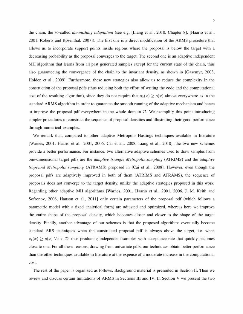
the chain, the so-called diminishing adaptation (see e.g. [Liang et al., 2010, Chapter 8], [Haario et al.,

2001, Roberts and Rosenthal, 2007]). The first one is a direct modification of the ARMS procedure that

allows us to incorporate support points inside regions where the proposal is below the target with a

decreasing probability as the proposal converges to the target. The second one is an adaptive independent

MH algorithm that learns from all past generated samples except for the current state of the chain, thus

also guaranteeing the convergence of the chain to the invariant density, as shown in [Gasemyr, 2003,

Holden et al., 2009]. Furthermore, these new strategies also allow us to reduce the complexity in the

construction of the proposal pdfs (thus reducing both the effort of writing the code and the computational

cost of the resulting algorithm), since they do not require that πt(x) ≥ p(x) almost everywhere as in the

standard ARMS algorithm in order to guarantee the smooth running of the adaptive mechanism and hence

to improve the proposal pdf everywhere in the whole domain D. We exemplify this point introducing

simpler procedures to construct the sequence of proposal densities and illustrating their good performance

through numerical examples.

We remark that, compared to other adaptive Metropolis-Hastings techniques available in literature

[Warnes, 2001, Haario et al., 2001, 2006, Cai et al., 2008, Liang et al., 2010], the two new schemes

provide a better performance. For instance, two alternative adaptive schemes used to draw samples from

one-dimensional target pdfs are the adaptive triangle Metropolis sampling (ATRIMS) and the adaptive

trapezoid Metropolis sampling (ATRAMS) proposed in [Cai et al., 2008]. However, even though the

proposal pdfs are adaptively improved in both of them (ATRIMS and ATRAMS), the sequence of

proposals does not converge to the target density, unlike the adaptive strategies proposed in this work.

Regarding other adaptive MH algorithms [Warnes, 2001, Haario et al., 2001, 2006, J. M. Keith and

Sofronov, 2008, Hanson et al., 2011] only certain parameters of the proposal pdf (which follows a

parametric model with a fixed analytical form) are adjusted and optimized, whereas here we improve

the entire shape of the proposal density, which becomes closer and closer to the shape of the target

density. Finally, another advantage of our schemes is that the proposed algorithms eventually become

standard ARS techniques when the constructed proposal pdf is always above the target, i.e. when

πt(x) ≥ p(x) ∀x ∈ D, thus producing independent samples with acceptance rate that quickly becomes

close to one. For all these reasons, drawing from univariate pdfs, our techniques obtain better performance

than the other techniques available in literature at the expense of a moderate increase in the computational

cost.

The rest of the paper is organized as follows. Background material is presented in Section II. Then we

review and discuss certain limitations of ARMS in Sections III and IV. In Section V we present the two

6

novel techniques, whereas alternative procedures to construct the proposal pdf are described in Section

VI. Finally, numerical simulations are shown in Section VII and conclusions are drawn in Section VIII.

II. BACKGROUND

A. Notation

We indicate random variables with upper-case letters, e.g. X , while we use lower-case letters to denote

the corresponding realizations, e.g. x. Sets are denoted with calligraphic upper-case letters, e.g. R. The

domain of the variable of interest, x, is denoted as D ⊆ R. The normalized target PDF is indicated

as po(x), whereas p(x) = cppo(x) represents the unnormalized target. The normalized proposal PDF is

denoted as π(x), whereas π(x) = cππ(x) is the unnormalized proposal. For simplicity, we also refer

to the unnormalized functions p(x) and π(x), and in general to all unnormalized but proper PDFs, as

densities.

B. Adaptive rejection sampling

The standard adaptive rejection sampling (ARS) algorithm [Gilks, 1992, Gilks and Wild, 1992, Gilks

et al., 1997] enables the construction of a sequence of proposal densities, {πt(x)}t∈N, tailored to the

target density, po(x) ∝ p(x). Its most appealing feature is that each time that a sample is drawn from a

proposal, πt(x), and it is rejected, this sample can be used to build an improved proposal, πt+1(x), with a

higher mean acceptance rate. Unfortunately, the ARS method can only be applied with target pdfs which

are log-concave (and thus unimodal), which is a very stringent constraint for many practical applications

[Gilks et al., 1995b, Martino and Mıguez, 2011]. In this section we briefly review the ARS algorithm,

which is the basis for the ARMS method and the subsequent improvements proposed in this paper.

Let us assume that we want to draw samples from a target pdf, po(x) ∝ p(x), with support D ⊆ R,

known up a normalization constant. The ARS procedure can be applied when p(x) is log-concave, i.e.

when

V (x) , log(p(x)), (1)

is strictly concave ∀x ∈ D ⊆ R. In this case, let

St , {s1, s2, . . . , smt} ⊂ D (2)

be the set of support points at time t, sorted in ascending order (i.e. s1 < . . . < smt). Note that the

number of points mt can grow with the iteration index t. From St a piecewise-linear function Wt(x) is

7

constructed such that

Wt(x) ≥ V (x), (3)

for all x ∈ D and ∀t ∈ N. Different approaches are possible for constructing this function. For instance,

if we denote by wk(x) the linear function tangent to V (x) at sk ∈ St [Gilks and Wild, 1992], then a

suitable piecewise linear function Wt(x) is:

Wt(x) , min{w1(x), . . . , wmt(x)} for x ∈ D. (4)

In this case, clearly we have Wt(x) ≥ V (x), ∀x ∈ D and ∀t ∈ N, as shown in Figure 1(a). However,

it is also possible to construct Wt(x) without using the first derivative of V (x), which is involved in

the calculation of the tangent lines used in the previous approach, by using secant lines [Gilks, 1992].

Indeed, defining the intervals

I0 , (−∞, s1], I1 , (s1, s2], ... Ij , (sj , sj+1], ..., Imt, (smt−1, smt

], Imt, (smt

,+∞) (5)

and denoting as Li,i+1(x) the straight line passing through the points (si, V (si)) and (si+1, V (si+1)) for

1 ≤ i ≤ mt, a suitable function Wt(x) can be expressed as

Wt(x) ,

L1,2(x), x ∈ I0 = (−∞, s1];

L2,3(x), x ∈ I1 = (s1, s2];

min{Lj−1,j(x), Lj+1,j+2(x)}, x ∈ Ij = (sj , sj+1], 2 ≤ j ≤ mt − 2;

Lmt−2,mt−1(x), x ∈ Imt−1 = (smt−1, smt];

Lmt−1,mt(x), x ∈ Imt

= (smt,+∞).

(6)

It is apparent also in this case that Wt(x) ≥ V (x), ∀x ∈ D and ∀t ∈ N, as shown in Figure 1(b).

Therefore, building Wt(x) such that Wt(x) ≥ V (x), we have in both cases

πt(x) , exp(Wt(x)) ≥ p(x) = exp{V (x)}. (7)

Since Wt(x) is a piecewise linear function, we obtain an exponential-type proposal density, πt(x) ∝ πt(x).

Note also that knowledge of the area below each exponential piece, ki =∫x∈Ii exp(Wt(x))dx for

0 ≤ i ≤ mt, is required to generate samples from πt(x), and, given the functional form of πt(x), it

is straightforward to compute each of these terms, as well as the normalization constant, 1/cπ with

cπ =∫x∈D πt(x)dx, since cπ = k0 + k2 + ...+ kn.

Therefore, we conclude that, since πt(x) is a piecewise-exponential function, it is very easy to

draw samples from πt(x) = 1cππt(x) and, since πt(x) ≥ p(x), we can apply the rejection sampling

8

principle. Moreover, when a sample x′ drawn from πt(x) is rejected, we can incorporate it into the

set of support points, i.e. St+1 = St ∪ {x′} and mt+1 = mt + 1. Then, we can compute a refined

approximation, Wt+1(x), following one of the two approaches described above, and a new proposal

density, πt+1(x) = exp(Wt+1(x)), can be constructed. Table I summarizes the procedure followed by

the ARS algorithm to generate N samples from a target p(x).

TABLE I

ADAPTIVE REJECTION SAMPLING ALGORITHM.

1. Start with i = 0, t = 0, m0 = 2, S0 = {s1, s2} where s1 < s2 and [s1, s2] contains the mode.

Let N be the number of desired samples from po(x) ∝ p(x).

2. Build the piecewise-linear function Wt(x) as in Eq. (4) or (6), and as shown in Figure 1(a) or 1(b).

3. Sample x′ from πt(x) ∝ πt(x) = exp(Wt(x)), and u′ from U([0, 1]).

4. If u′ ≤ p(x′)πt(x)

then accept x(i) = x′ and set St+1 = St (mt+1 = mt), i = i+ 1.

5. Otherwise, if u′ > p(x′)πt(x′)

, then reject x′, set St+1 = St ∪ {x′} (mt+1 = mt + 1).

6. Sort St+1 in ascending order and set t = t+ 1. If i = N , then stop. Else, go back to step 2.

It is important to observe that the adaptive strategy followed by ARS includes new support points

only when and where they are needed, i.e. when a sample is rejected, indicating that the discrepancy

between the shape of the target and the proposal pdfs is potentially large. This discrepancy is measured

by computing the ratio p(x)/πt(x). Since πt(x) approaches p(x) when t → ∞, the ratio p(x)/πt(x)

becomes closer and closer to one, and the probability of adding a new support point becomes closer

and closer to zero, thus ensuring that the computational cost remains bounded. More details about the

convergence of ARS are provided below.

C. Convergence

Note that every time a sample x′ drawn from πt(x) is rejected, x′ is incorporated as a support point in

the new set St+1 = St ∪ {x′}. As a consequence, a refined lower hull Wt+1(x) is constructed, yielding

a better approximation of the system’s potential function, V (x). In this way, πt+1(x) = exp(Wt+1(x))

becomes “closer” to p(x) and the mean acceptance rate can be expected to become higher. More precisely,

the probability of accepting a sample x ∈ D drawn from πt(x) is

at(x) ,p(x)

πt(x), (8)

9

€

s1

€

s2

€

s3

€

w1(x)€

w2 (x)

€

w3(x)

€

V (x)

€

Wt (x)

(a)

€

V (x)

€

s1

€

s2

€

s3

€

Wt (x)

€

s4

€

s5

(b)

Fig. 1. Two possible procedures to build a suitable piecewise linear function Wt(x) ≥ V (x) when V (x) is concave: (a) using

the first derivative of V (x) (i.e. tangent lines) at the support points (with 3 support points, for instance); (b) using secant lines

(with 5 support points, for instance).

and we define the acceptance rate at the t-th iteration of the ARS algorithm, denoted as at, as the expected

value of at(x) with respect to the normalized pdf πt(x), i.e.,

at , E[at(x)] =

∫Dat(x)πt(x)dx =

∫D

p(x)

πt(x)πt(x)dx =

1

cπ

∫Dp(x)dx =

cpcπ≤ 1, (9)

where 1/cπ and 1/cp are the proportionality constants for πt(x) and p(x) respectively, i.e.

cπ =

∫Dπt(x)dx,

and

cp =

∫Dp(x)dx,

and we remark that cpcπ≤ 1 because πt(x) ≥ p(x) ∀x ∈ D. Hence, from (9) we conclude that

at = 1⇔ cπ = cp. Equivalently, defining the distance between two curves Dπ|p(t) as

Dπ|p(t) ,∫D|πt(x)− p(x)| dx =

∫D|exp(Wt(x))− exp(V (x))| dx, (10)

then we have at = 1⇔ Dπ|p(t) = 0. Note that this distance Dπ|p(t) measures the discrepancy between

the proposal πt(x) and the target p(x) pdfs. In particular, if Dπ|p(t) decreases the acceptance rate at =cpcπ

increases, and, since exp(Wt(x)) ≥ exp(V (x)) ∀x ∈ D, Dπ|p(t) = 0 if, and only if, Wt(x) = V (x)

almost everywhere. Equivalently, at = 1 if, and only if, πt(x) = p(x) almost everywhere.

10

III. ADAPTIVE REJECTION METROPOLIS SAMPLING ALGORITHM

The disadvantage of the classical ARS technique is that it can only draw samples from univariate log-

concave densities. In general, for non-log-concave and multimodal pdfs it is difficult to build a function

Wt(x) that satisfies the condition Wt(x) ≥ V (x) for all x ∈ D. Recognizing this problem, in [Gilks

et al., 1995b] an extension of ARS is suggested to deal with pdfs that are not log-concave by appending a

Metropolis-Hastings (MH) algorithm step [Hastings, 1970, Metropolis et al., 1953, Metropolis and Ulam,

1949]. The adaptive rejection Metropolis sampling (ARMS) first performs an RS test, and the discarded

samples are used to improve the proposal pdf, as in the standard ARS technique. However, if the sample

is accepted in the RS test, then the ARMS adds another statistical control using the MH acceptance

rule. This guarantees that the accepted samples are distributed according to the target pdf, p(x), even if

Wt(x) < V (x). Therefore, unlike ARS, the algorithm produces a Markov chain and the resulting samples

are correlated. Finally, we remark that the ARMS technique can be seen as an adaptive generalization of

the rejection sampling chain proposed in [Tierney, 1991, 1994].

The ARMS algorithm is described in detail in Table II. The time index k denotes the iteration of the

chain whereas t is the index corresponding to evolution of the sequence of proposal pdfs {πt(x)}t∈N.

The key stages are steps 4 and 5. On the one hand, in step 4 of Table II, when a sample is rejected

by the RS test (it is possible if and only if πt(x′) > p(x′)), ARMS adds this new point to the set Stand uses it to improve the construction of Wt+1(x) and go back to step 2. On the other hand, when a

sample is initially accepted by the RS test (clearly this always happens if πt(x′) < p(x′)), ARMS enters

in step 5 and uses the MH acceptance rule to determine whether it is finally accepted or not. However,

notice that ARMS never incorporates this new point to St, even if it is finally rejected by the MH step.

Observe also that, if πt(x) ≥ p(x) ∀x ∈ D and ∀t ∈ N, then the ARMS becomes the standard ARS

scheme, since the proposed sample is always accepted in step 5.

Moreover, since πt(x) depends on the support points, a more rigorous notation would be πt(x|St).

However, since St never contains the current state of the chain, then the ARMS can be considered an

adaptive independent MH algorithm and, for this reason, the dependence on St is usually omitted from

the notation. Indeed, the ARMS can be also seen as a particular case of the auxiliary variables method

in [Besag and Green, 1993].

Finally, we observe that, although in [Gilks et al., 1995b] the ARMS algorithm seems to be tightly

linked to a particular mechanism to construct the sequence of the proposal pdfs, in fact these two issues

can be studied separately. Therefore, in the following section we describe the two procedures proposed

11

in literature to construct the function Wt(x) in a suitable way [Gilks et al., 1995b, Meyer et al., 2008].

TABLE II

ADAPTIVE REJECTION METROPOLIS SAMPLING ALGORITHM.

1. Start with k = 0 (iteration of the chain), t = 0, S0 = {s1, . . . , sm0}, with s1 < s2 < . . . < sm0 ,

and choose a value x0. Let N be the required number of iterations of the Markov chain.

2. Build a function Wt(x) using the set of points St and one of the two procedures described in Section III-A

[Gilks et al., 1995b, Meyer et al., 2008].

3. Sample x′ from πt(x) ∝ πt(x) = exp(Wt(x)), and u′ from U([0, 1]).

4. If u′ > p(x′)πt(x′)

, then discard x′, set St+1 = St ∪ {x′}, mt+1 = mt + 1, sort St+1 in ascending order,

update t = t+ 1, and go back to step 2.

5. Otherwise, i.e. if u′ ≤ p(x′)πt(x′)

, set xk+1 = x′ with probability

α = min[1, p(x

′)min[p(xk),πt(xk)]p(xk)min[p(x′),πt(x′)]

],

or set xk+1 = xk with probability 1− α. Moreover, set St+1 = St, mt+1 = mt, t = t+ 1 and k = k + 1.

6. If k = N − 1, then stop. Else, go back to step 2.

A. Procedure to build Wt(x) proposed in [Gilks et al., 1995b]

Consider again a set of support points St = {s1, ..., smt} and the mt + 1 intervals I0 = (−∞, s1],

Ij = (sj , sj+1], for j = 1, ...,mt − 1 and Imt= (smt

,+∞). Moreover, let us denote as Lj,j+1(x) the

straight line passing through the points (sj , V (sj)) and (sj+1, V (sj+1)) for j = 1, ...,mt − 1, and also

set

L−1,0(x) = L0,1(x) , L1,2(x),

Lmt,mt+1(x) = Lmt+1,mt+2(x) , Lmt−1,mt(x).

In the standard ARMS procedure introduced in [Gilks et al., 1995b], the function Wt(x) is piecewise

linear and defined as

Wt(x) = max[Li,i+1(x),min [Li−1,i(x), Li+1,i+2(x)]

]for Ii = (si, si+1], (11)

with i = 0, . . . ,mt. The function Wt(x) can be also rewritten in a more explicit form as

Wt(x) =

L1,2(x), x ∈ I0 = (−∞, s1];

max {L1,2(x), L2,3(x)} , x ∈ I1 = (s1, s2];

max {Lj,j+1(x),min {Lj−1,j(x), Lj+1,j+2(x)}} , x ∈ Ij = (sj , sj+1], 2 ≤ j ≤ mt − 2;

max {Lmt−1,mt(x), Lmt−2,mt−1(x)} , x ∈ Imt−1 = (smt−1, smt

];

Lmt−1,mt(x), x ∈ Imt = (smt ,+∞).

(12)

12

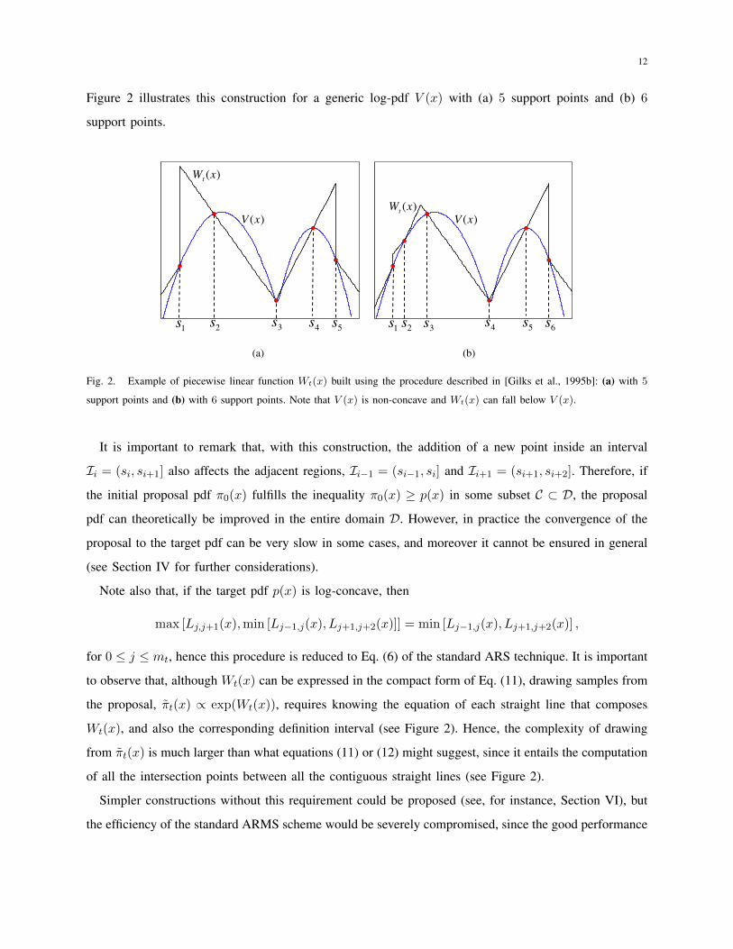
Figure 2 illustrates this construction for a generic log-pdf V (x) with (a) 5 support points and (b) 6

support points.

€

V (x)€

Wt (x)

€

s1

€

s2

€

s3

€

s4

€

s5

(a)

€

V (x)

€

Wt (x)

€

s1

€

s3

€

s4

€

s5

€

s6

€

s2

(b)

Fig. 2. Example of piecewise linear function Wt(x) built using the procedure described in [Gilks et al., 1995b]: (a) with 5

support points and (b) with 6 support points. Note that V (x) is non-concave and Wt(x) can fall below V (x).

It is important to remark that, with this construction, the addition of a new point inside an interval

Ii = (si, si+1] also affects the adjacent regions, Ii−1 = (si−1, si] and Ii+1 = (si+1, si+2]. Therefore, if

the initial proposal pdf π0(x) fulfills the inequality π0(x) ≥ p(x) in some subset C ⊂ D, the proposal

pdf can theoretically be improved in the entire domain D. However, in practice the convergence of the

proposal to the target pdf can be very slow in some cases, and moreover it cannot be ensured in general

(see Section IV for further considerations).

Note also that, if the target pdf p(x) is log-concave, then

max [Lj,j+1(x),min [Lj−1,j(x), Lj+1,j+2(x)]] = min [Lj−1,j(x), Lj+1,j+2(x)] ,

for 0 ≤ j ≤ mt, hence this procedure is reduced to Eq. (6) of the standard ARS technique. It is important

to observe that, although Wt(x) can be expressed in the compact form of Eq. (11), drawing samples from

the proposal, πt(x) ∝ exp(Wt(x)), requires knowing the equation of each straight line that composes

Wt(x), and also the corresponding definition interval (see Figure 2). Hence, the complexity of drawing

from πt(x) is much larger than what equations (11) or (12) might suggest, since it entails the computation

of all the intersection points between all the contiguous straight lines (see Figure 2).

Simpler constructions without this requirement could be proposed (see, for instance, Section VI), but

the efficiency of the standard ARMS scheme would be severely compromised, since the good performance

13

of ARMS depends critically on the construction of the proposal, as discussed in the following section

and shown in the simulations (see Section VII).

Another possible and more complex procedure for building Wt(x) was proposed in [Meyer et al.,

2008], involving quadratic approximations of the log-pdf V (x) when it is possible, so that the proposal

is also formed by truncated Gaussian pdfs. Indeed, parabolic pieces passing through 3 support points

are used if only if the resulting quadratic function is concave (in order to obtain truncated Gaussian as

proposal pdf in the corresponding interval). Otherwise, linear functions are used to build Wt(x). The main

advantage of this alternative procedure [Meyer et al., 2008] is that it provides a better approximation of

the function V (x) = log(p(x)). However, it does not overcome the critical structural limitation of the

standard ARMS technique that we explain in the sequel.

IV. STRUCTURAL LIMITATION IN THE ADAPTIVE PROCEDURE OF ARMS

Although ARMS can be a very effective technique for sampling from univariate non-log-concave pdfs,

its performance depends critically on the following two issues:

a) The construction of Wt(x) should be such that the condition Wt(x) ≥ V (x) is satisfied for

most intervals x ∈ Ij as possible, with j = 0, 1, . . . , mt. That is, the proposal function

πt(x) = exp(−Wt(x)) must stay above the target pdf p(x), inside as many intervals as possible,

covering as much of the domain D as possible. In this case the adaptive procedure works almost

in the entire domain D and the proposal density can be improved virtually everywhere. Indeed, if

πt(x) ≥ p(x) for all x ∈ D and for all t ∈ N, the ARMS is reduced the classical ARS algorithm.

b) The addition of a support point within an interval, Ij = (sj , sj+1], with j ∈ {0, ...,mt}, must entail

an improvement of the proposal pdf inside other neighboring intervals when building Wt+1(x). This

allows the proposal pdf to improve even inside regions where πt(x) < p(x) and a support point

can never be added at the t-th iteration, since we could have πt+1(x) > p(x) by adding a support

point in an adjacent interval. For instance, in the procedure described in Section III-A [Gilks et al.,

1995b], when a support point is added inside Ij , the proposal pdf also changes in the intervals

Ij−1 and Ij+1. Consequently, the drawback of not adding support points within the intervals where

πt(x) < p(x) is reduced, but may not completely eliminated, as shown through an example below.

In any case, it is important to remark that the convergence of the proposal πt(x) to the target pdf

p(x), cannot be guaranteed using any suitable construction of Wt(x) except for the special case where

Wt(x) ≥ V (x) ∀x ∈ D and ∀t ∈ N, where ARMS is reduced to ARS. This is due to a fundamental

14

structural limitation of the ARMS technique caused by the impossibility of adding support points inside

regions where πt(x) < p(x).

Indeed, it is possible that inside some region C ⊂ D where πt(x) < p(x), we obtain a sequence of

proposals {πt+1(x), πt+2(x), . . . , πt+τ (x)} such that πt+1(x) < p(x), πt+2(x) < p(x), . . . , πt+τ (x) <

p(x) for an arbitrarily large value of τ , and the discrepancy between the proposal and the target pdfs

cannot be reduced after an iteration t = τ , clearly implying that the proposal does not converge to the

target for x ∈ D.

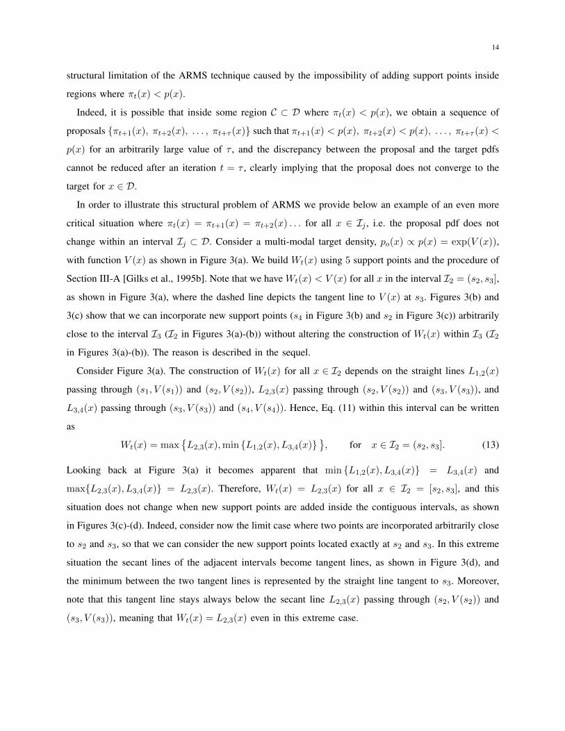
In order to illustrate this structural problem of ARMS we provide below an example of an even more

critical situation where πt(x) = πt+1(x) = πt+2(x) . . . for all x ∈ Ij , i.e. the proposal pdf does not

change within an interval Ij ⊂ D. Consider a multi-modal target density, po(x) ∝ p(x) = exp(V (x)),

with function V (x) as shown in Figure 3(a). We build Wt(x) using 5 support points and the procedure of

Section III-A [Gilks et al., 1995b]. Note that we have Wt(x) < V (x) for all x in the interval I2 = (s2, s3],

as shown in Figure 3(a), where the dashed line depicts the tangent line to V (x) at s3. Figures 3(b) and

3(c) show that we can incorporate new support points (s4 in Figure 3(b) and s2 in Figure 3(c)) arbitrarily

close to the interval I3 (I2 in Figures 3(a)-(b)) without altering the construction of Wt(x) within I3 (I2in Figures 3(a)-(b)). The reason is described in the sequel.

Consider Figure 3(a). The construction of Wt(x) for all x ∈ I2 depends on the straight lines L1,2(x)

passing through (s1, V (s1)) and (s2, V (s2)), L2,3(x) passing through (s2, V (s2)) and (s3, V (s3)), and

L3,4(x) passing through (s3, V (s3)) and (s4, V (s4)). Hence, Eq. (11) within this interval can be written

as

Wt(x) = max{L2,3(x),min {L1,2(x), L3,4(x)}

}, for x ∈ I2 = (s2, s3]. (13)

Looking back at Figure 3(a) it becomes apparent that min {L1,2(x), L3,4(x)} = L3,4(x) and

max{L2,3(x), L3,4(x)} = L2,3(x). Therefore, Wt(x) = L2,3(x) for all x ∈ I2 = [s2, s3], and this

situation does not change when new support points are added inside the contiguous intervals, as shown

in Figures 3(c)-(d). Indeed, consider now the limit case where two points are incorporated arbitrarily close

to s2 and s3, so that we can consider the new support points located exactly at s2 and s3. In this extreme

situation the secant lines of the adjacent intervals become tangent lines, as shown in Figure 3(d), and

the minimum between the two tangent lines is represented by the straight line tangent to s3. Moreover,

note that this tangent line stays always below the secant line L2,3(x) passing through (s2, V (s2)) and

(s3, V (s3)), meaning that Wt(x) = L2,3(x) even in this extreme case.

15

€

V (x)

€

Wt (x)

€

s1

€

s3

€

s4

€

s5

€

s2

(a)

€

V (x)

€

Wt (x)

€

s1

€

s3

€

s5

€

s6

€

s2

€

s4

(b)

€

V (x)

€

s1

€

s4

€

s6

€

s7

€

s2

€

s5

€

s3

€

Wt (x)

(c)

€

V (x)

€

s2

€

s3

(d)

Fig. 3. Example of a critical structural limitation in the adaptive procedure of the ARMS. (a) Construction of Wt(x) with 5

support points. Within I2 = (s2, s3] we have Wt(x) < V (x). (b)-(c) Adding new support points inside the contiguous intervals

the construction of Wt(x) does not vary within I2 (I3 in Figure (c)). (d) The secant line L2,3(x) passing through (s2, V (s2))

and (s3, V (s3)), and the two tangent lines to V (x) at s2 and s3.

Therefore, with the adaptive procedure used by the standard ARMS technique to build the proposal

pdf, the function Wt(x) could remain unchanged in a subset of the entire domain D that contains a

mode of the target pdf, as shown in the previous example. Hence, the discrepancy between the proposal

πt(x) = exp(Wt(x)) and the target p(x) = exp(V (x)), is not reduced at all, as t→ +∞.

A trivial solution for this drawback of the standard ARMS algorithm could be adding new support

points within the set St each time that the MH step in the ARMS (step 5) is applied. Unfortunately, from

a practical point of view the first problem of this approach is the unbounded increase in computational

cost since the number of points in St grows indefinitely. Another major problem from a theoretical point

of view is that the convergence of the Markov chain to the invariant pdf cannot be ensured in this case,

16

since the current state of the chain could be contained in St (see [Liang et al., 2010, Chapter 8], [Holden

et al., 2009] for a discussion of this issue).

For these two reasons in the following section we propose two variants of the standard ARMS technique

that ensure the convergence of the Markov chain to the target density while keeping the computational

cost bounded and low.

V. VARIANTS OF THE ARMS ALGORITHM

In this section we describe two alternative strategies to improve the standard ARMS algorithm. We

denote these two variants as A2RMS and IA2RMS where the A2 emphasizes that we incorporate an

additional adaptive step to improve the proposal density w.r.t. the standard ARMS. Note that in this

section we use the more rigorous notation for the proposal, πt(x|St) instead of simply πt(x), for clarity

with respect to the convergence of the Markov chain.

A. First scheme: A2RMS

A first possible enhancement of the ARMS technique is summarized below. The basic underlying

idea is enhancing the performance of ARMS by introducing the possibility of adding a sample to the

support set even when it is initially accepted by the RS test. The procedure followed allows A2RMS

to incorporate support points inside regions where πt(x|St) < p(x) in a controlled way (i.e. with a

decreasing probability as the Markov chain evolves), thus ensuring the convergence to the target and

preventing the computational cost from growing indefinitely.

The steps taken by the A2RMS algorithm are the following:

1. Set k = 0 (iteration of the chain), t = 0, choose an initial value x0 and the time to stop the

adaptation, K. Let N > K be the needed number of iterations of the Markov chain.

2. Given a set of support points, St = {s1, . . . , smt} such that s1 < s2 < . . . < smt

, build an

approximation Wt(x) of the potential function V (x) = log (p(x)) using a convenient procedure

(e.g. the ones described in [Gilks et al., 1995b, Meyer et al., 2008] or the simpler ones proposed in

Section VI).

3. Draw a sample x′ from πt(x|St) ∝ πt(x|St) = exp(Wt) and another sample from u′ ∼ U([0, 1]).

4. If u′ > p(x′)πt(x′|St) , then discard x′, set St+1 = St ∪ {x′}, mt+1 = mt + 1, sort St+1 in ascending

order, update t = t+ 1, and go back to step 2.

5. If u′ ≤ p(x′)πt(x′|St) , then:

17

5.1. Set xk+1 = x′ with probability

α = min

[1,p(x′)min[p(xk), πt(xk|St)]p(xk)min[p(x′), πt(x′|St)]

], (14)

or xk+1 = xk with probability 1− α.

5.2. If k ≤ K, draw u2 ∼ U([0, 1]) and if

u2 >πt(x

′|St)p(x′)

,

set St+1 = St∪{x′}, mt+1 = mt+1 and sort St+1 in ascending order. Otherwise, set St+1 = St,

mt+1 = mt.

5.3. Update t = t+ 1 and k = k + 1.

6. If k < N , go back to step 2.

We remark again that the key point in the A2RMS algorithm is that, due to the introduction of step

5.2 w.r.t. the ARMS, new support points can also added inside the regions of the domain D where

πt(x|St) < p(x). Note that, when πt(x′|St) ≥ p(x′) and we accept the proposed sample x′ in the

RS test, then we also apply the MH acceptance rule and always accept x′, as α = 1, but we never

incorporate x′ to the set of support points, since πt(x′|St)p(x′) ≥ 1 and u2 ∼ U([0, 1]). Therefore, if the

condition πt(x|St) ≥ p(x) is satisfied in all the domain x ∈ D, then the A2RMS is reduced to the

standard ARS, just like it happens for ARMS.

It is important to remark that the effort to code and implement the algorithm is virtually unchanged.

Moreover, the ratio πt(x′|St)p(x′) = 1

p(x′)πt(x

′|St)

in the step 5.2 is already calculated in the RS control (steps 4

and 5), hence it is not necessary to evaluate the proposal and the target pdfs again.

Since it is difficult to guarantee that the Markov chain converge to the target pdf, po(x) ∝ p(x), we

have introduced a time K to stop the second adaptation step 5.2. Therefore, theoretically the first K

samples produced by the algorithm should be discarded. Observe that for k > K the A2RMS coincides

to the standard ARMS.

The issue with the convergence of the chain is due to the fact that we are incorporating the current state

xt, into the set of support points St, on which the proposal depends. Therefore, the balance condition

using the acceptance function in Eq. (14) could be not satisfied for k ≤ K and those first K samples could

be seen just as auxiliary random variables obtained as part of the process to construct a good proposal

pdf, and thus should be removed from the set of final returned samples. However, it is important to notice

the following two facts:

a) It is a common practice with MCMC techniques to remove a certain amount of the firstly generated

samples in order to diminish the effect of the so called burn-in period.

18

b) We have found out empirically that, even if we set K = N and use all the samples produced by

the Markov chain, the A2RMS algorithm also provides very good results, as we show in Section

VII. Indeed, the probability of incorporating new support points quickly tends to zero as t increases,

effectively vanishing as t→ +∞. This is due to the fact that, each time that a new point is added,

the proposal density is improved and becomes closer and closer to the target pdf in the whole

domain D. Therefore, the two ratios p(x)πt(x|St) and πt(x|St)

p(x) approach one and the probability of adding

a new support point becomes arbitrarily close to zero. This implies that the computational cost of

the algorithm remains bounded, i.e. a very good approximation of the target can be obtained with

a finite number of support points adaptively chosen.

Hence, A2RMS satisfies the first condition needed to ensure the convergence of the Markov chain to the

target pdf, known as diminishing adaptation (see [Liang et al., 2010, Chapter 8], [Haario et al., 2001,

Roberts and Rosenthal, 2007]). Unfortunately, it is difficult to assert whether the A2RMS with K = N

also fulfills the second condition needed to guarantee the convergence of the chain, called bounded

convergence [Liang et al., 2010, Chapter 8]. For this reason, although the good results obtained in the

numerical simulations with K = N (see Section VII) lead us to believe that convergence occurs, it may

be safer to set K < N in order to avoid convergence problems in practical applications.

Furthermore, in the next section we introduce a second A2RMS scheme for which convergence to the

target can be ensured, since it is an adaptive independent MH algorithm [Gasemyr, 2003, Holden et al.,

2009].

B. Second scheme: Independent A2RMS (IA2RMS)

A second possible improvement of ARMS is an adaptive independent MH algorithm that we indicate as

IA2RMS. The main modification of IA2RMS w.r.t. A2RMS is building the proposal pdf using possibly

all the generated past samples but without taking into account the current state xt of the chain. The

IA2RMS is described in the following.

1. Set k = 0 (iteration of the chain), t = 0 and choose an initial value x0.

2. Given a set of support points, St = {s1, . . . , smt}, such that s1 < s2 < . . . < smt

, build an

approximation Wt(x) of the function V (x) = log (p(x)) using a convenient procedure (e.g. the ones

described in [Gilks et al., 1995b, Meyer et al., 2008] or the simpler ones proposed in Section VI).

3. Draw a sample x′ from πt(x|St) ∝ πt(x|St) = exp(Wt) and another sample from u′ ∼ U([0, 1]).

4. If u′ > p(x′)πt(x′|St) , then discard x′, set St+1 = St ∪ {x′} and mt+1 = mt + 1, sort St+1 in ascending

order, update t = t+ 1 and go back to step 2.

19

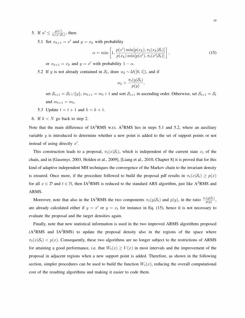
5. If u′ ≤ p(x′)πt(x′|St) , then:

5.1 Set xk+1 = x′ and y = xk with probability

α = min

[1,p(x′)min[p(xk), πt(xk|St)]p(xk)min[p(x′), πt(x′|St)]

], (15)

or xk+1 = xk and y = x′ with probability 1− α.

5.2 If y is not already contained in St, draw u2 ∼ U([0, 1]), and if

u2 >πt(y|St)p(y)

,

set St+1 = St∪{y}, mt+1 = mt+1 and sort St+1 in ascending order. Otherwise, set St+1 = Stand mt+1 = mt.

5.3 Update t = t+ 1 and k = k + 1.

6. If k < N go back to step 2.

Note that the main difference of IA2RMS w.r.t. A2RMS lies in steps 5.1 and 5.2, where an auxiliary

variable y is introduced to determine whether a new point is added to the set of support points or not

instead of using directly x′.

This construction leads to a proposal, πt(x|St), which is independent of the current state xt of the

chain, and in [Gasemyr, 2003, Holden et al., 2009], [Liang et al., 2010, Chapter 8] it is proved that for this

kind of adaptive independent MH techniques the convergence of the Markov chain to the invariant density

is ensured. Once more, if the procedure followed to build the proposal pdf results in πt(x|St) ≥ p(x)

for all x ∈ D and t ∈ N, then IA2RMS is reduced to the standard ARS algorithm, just like A2RMS and

ARMS.

Moreover, note that also in the IA2RMS the two components πt(y|St) and p(y), in the ratio πt(y|St)p(y) ,

are already calculated either if y = x′ or y = xt for instance in Eq. (15), hence it is not necessary to

evaluate the proposal and the target densities again.

Finally, note that new statistical information is used in the two improved ARMS algorithms proposed

(A2RMS and IA2RMS) to update the proposal density also in the regions of the space where

πt(x|St) < p(x). Consequently, these two algorithms are no longer subject to the restrictions of ARMS

for attaining a good performance, i.e. that Wt(x) ≥ V (x) in most intervals and the improvement of the

proposal in adjacent regions when a new support point is added. Therefore, as shown in the following

section, simpler procedures can be used to build the function Wt(x), reducing the overall computational

cost of the resulting algorithms and making it easier to code them.

20

VI. ALTERNATIVE PROCEDURES TO BUILD πt(x)

As discussed before, the improvements proposed in the structure of the standard ARMS allow us to

use simpler procedures to construct the function Wt(x).

For instance, a first approach inspired by the one used in ARMS is defining Wt(x) inside the i-th

interval as the straight line going through (si, V (si)) and (si+1, V (si+1)), Li,i+1(x), for 1 ≤ i ≤ mt−1,

and extending the straight lines corresponding to I1 and Imt−1 towards minus and plus infinity for the

first and last intervals, I0 and Imtrespectively. Mathematically, this can be expressed as

Wt(x) =

L1,2(x), x ∈ I0 = (−∞, s1];

Li,i+1(x), x ∈ Ii = (si, si+1], 1 ≤ i ≤ mt − 1;

Lmt−1,mt(x), x ∈ Imt

= (smt,+∞).

(16)

This is illustrated in Figure 4(a). Note that, although this procedure looks similar to the one used in ARMS,

as described by Eqs. (11) and (12), it is much simpler in fact, since there is not any minimization or

maximization involved, and thus it does not require the calculation of intersection points to determine

when one straight line is above the other.

Moreover, an even simpler procedure to construct Wt(x) can be devised from (16): using a piecewise

constant approximation with two straight lines inside the first and last intervals. Mathematically, it can

be expressed as

Wt(x) =

L1,2(x), x ∈ I0 = (−∞, s1];

max {V (si), V (si+1)} , x ∈ Ii = (si, si+1];

Lmt−1,mt(x), x ∈ Imt

= (smt,+∞).

(17)

The construction described above leads to the simplest proposal density possible, i.e., a collection of

uniform pdfs with two exponential tails. Figure 4(b) shows an example of the construction of the proposal

using this approach.

Note that, even when the target pdf is log-concave, using these two procedures the resulting ARMS-

type techniques are not reduced to standard ARS, since there is no guarantee that the resulting proposal

is above the target pdf. Indeed, when V (x) = log[p(x)] is concave, the first procedure described

by Eq. (17) will produce a proposal which is always below the target except inside the first and

last intervals. However, the second procedure described by Eq. (17) can be easily modified to yield

πt(x) = exp(Wt(x)) ≥ p(x) = exp(V (x)) ∀x ∈ D for log-concave target densities, if the position of the

mode is known or if an upper bound for V (x) is available and the location of the mode can be estimated

21

€

V (x)

€

s1

€

s3

€

s5

€

s2

€

s4

€

Wt (x)

(a)

€

V (x)

€

s1

€

s3

€

s5

€

s2

€

s4

€

Wt (x)

(b)

€

V (x)

€

s1

€

s3

€

s5

€

s2

€

s4

€

Wt (x)

€

B

(c)

Fig. 4. (a) Example of the construction of Wt(x) using the procedure described in Eq. (16). (b) Example of the construction

of Wt(x) using the procedure given by Eq. (17). (c) If the function V (x) is concave, the procedure in Eq. (17) can be modified

to obtain πt(x) ≥ p(x) for all x ∈ D. Indeed, this figure provides an example of the construction of Wt(x) when an upper

bound B ≥ V (x) is available and the location of the maximum can be estimated.

(e.g. using the sign of the first derivative). Figure 4(c) depicts an example of the construction of Wt(x)

when V (x) is concave using an upper bound B ≥ V (x) to obtain πt(x) ≥ p(x) ∀x ∈ D. Moreover,

it is important to remark that the procedure in Eq. (17), without any modifications, converges virtually

to produce πt(x) = exp(Wt(x)) ≥ p(x) = exp(V (x)) almost everywhere when V (x) is concave and

t→ +∞.

Finally, we note that we could also apply the procedures proposed for adaptive triangular Metropolis

sampling (ATRIMS) and adaptive trapezoid Metropolis sampling (ATRAMS) to build the proposal, even

though the structure of these two algorithms is completely different to ARMS [Cai et al., 2008]. In both

cases the proposal is constructed directly in the domain of the target pdf, p(x), rather than in the domain

of the log-pdf, V (x) = log(p(x)).

For instance, the basic idea proposed for ATRAMS is using straight lines, Li,i+1(x),2 passing through

the points (si, p(si)) and (si+1, p(si+1)) for i = 1, . . . ,mt − 1 and two exponential pieces, E0(x) and

Emt(x), for the tails:

πt(x) ∝ πt(x) =

E0(x), x ∈ I0 = (−∞, s1];

Li,i+1(x), x ∈ Ii = (si, si+1], i = 1, . . . ,mt − 1;

Emt(x), x ∈ Imt

= (smt,+∞).

(18)

2Note that we use the symbol ∼ to distinguish Li,i+1(x) and Li,i+1(x). Indeed, Li,i+1(x) is a straight line built directly in

the domain of p(x) whereas the linear function Li,i+1(x) is constructed in the log-domain.

22

Unlike in [Cai et al., 2008], here the tails E0(x) and Emt(x) do not necessarily have to be

equivalent in the areas they enclose. Indeed, we may follow a much simpler approach calculating two

secant lines L1,2(x) and Lmt−1,mt(x) passing through (s1, V (s1)), (s2, V (s2)), and (smt−1, V (smt−1)),

(smt, V (smt

)) respectively, so that the two exponential tails are defined as E0(x) = exp{L1,2(x)} and

Emt(x) = exp{Lmt−1,mt

(x)}.

Figure 5 depicts an example of the construction of πt(x) using this last procedure. Note that drawing

samples from these trapezoidal pdfs inside Ii = (si, si+1] can be easily done [Cai et al., 2008, Devroye,

1986]. Indeed, given u′, v′ ∼ U([si, si+1]) and w′ ∼ U([0, 1]), then

x′ =

min{u′, v′}, w′ < p(si)p(si)+p(si+1)

;

max{u′, v′}, w′ ≥ p(si)p(si)+p(si+1)

;

(19)

is distributed according to a trapezoidal density defined in the interval Ii = [si, si+1].

(a) (b)

Fig. 5. (a) Example of the construction of the proposal pdf, πt(x) ∝ πt(x), using a procedure described in [Cai

et al., 2008] within the ATRAMS algorithm. (b) The same construction in the log-domain, i.e. for V (x) = log(p(x)) and

Wt(x) = log(πt(x)).

All these procedures reduce the computational cost of the so called ARMS-type algorithms. However,

it is important to remark that they could be inefficient within the standard ARMS structure without the

proposed enhancements, as shown in Section VII and due to the reasons explained in Section III. An

important exception is the simple procedure described by Eq. (17), which leads to very good results

also in combination with the standard ARMS (although even better results are obtained for A2RMS and

IA2RMS), probably due to the fact that the proposal stays above the target almost everywhere.

23

A. Initial support points and tails

Depending on the type of construction, the minimum possible number m0 of initial support points

is at least 2 with the procedures described above or 3 with the procedure in [Gilks et al., 1995b]. In

general, to avoid numerical problems the user must only assure that p(s′) > 0 for at least one support

point s′. However, to speed up the convergence and render the algorithm more robust (avoiding any kind

of numerical problems), a greater number of support points can be used. Moreover, observe that there is

clearly a trade-off between the initial performance and overall computational cost.

It is important to note that the dependence on the choice of the set S0 can be reduced adding more

probability in the tails of the proposal PDF, initially. Indeed, consider the two slopes lt,1 and lt,2 of the

linear functions that form Wt(x) in I0 and Imt+1, constructed as explained above3. For instance, we can

add more probability in the tails of the proposal just by setting

l′t,1 = lt,1(1− βe−αt),

l′t,2 = lt,2(1− βe−αt),(20)

where 0 ≤ β ≤ 1, α > 0, and l′t,i → lti, i = 1, 2, for t→ +∞. Moreover, the proposed algorithms work

even if the target PDF has heavy tails on account of the second test in A2RMS and IA2RMS that allows

the incorporation of new support points where p(x) > πt(x|St). However, if we know what kind of tails

the target distribution has, we can speed up the convergence and reduce the burn-in period by changing

the construction of the tails of the proposal. For instance, we could use a function of type log[1/xγ ],

with γ > 1, to build Wt(x) in I0 and Imt+1, instead of straight lines.

VII. SIMULATIONS

In this section we compare the performance of the two proposed algorithms with the standard ARMS

scheme using four alternative procedures to build the proposal pdf πt(x) in all cases: the one proposed by

standard ARMS and described by Eq. (11) (procedure 1), the two simpler procedures given by Eqs. (16)

and (17) (procedures 2 and 3, respectively), and the procedure described in Eq. (18), which is adapted

from the ATRAM technique [Cai et al., 2008] (procedure 4).4

3Note that, in general, a control on the slopes lt,1 and lt,2 is needed to attain a proper proposal PDF since it is necessary

that lt,1 > 0 and lt,2 < 0.4Matlab code using the procedure in Eq. (17) to build the proposal is provided at http://a2rms.sourceforge.net/.

24

For the simulations, we consider a target pdf, po(x) ∝ p(x), generated as a mixture of 3 Gaussian

densities,

po(x) = 0.3N (x;−5, 1) + 0.3N (x; 1, 1) + 0.4N (x; 7, 1), (21)

where N(x;µ, σ2) denotes a Gaussian pdf with mean µ and variance σ2. In order to analyze the accuracy

of the different algorithms, we estimate the mean of po(x) using the generated samples, comparing it to

the true value, E{po(x)} = 1.6. Moreover, we also provide an estimation of the linear correlation among

consecutive samples of the Markov chain, an approximation of the distance Dπ|p(t) in Eq. (10) between

the constructed proposal and the target pdf, the number of rejections and the number of support points

at each iteration.

We consider N = 5000 iterations of the Markov chain and use an initial set S0 = {s1 = −10, s2 =

a, s3 = b, s4 = 10} formed by m0 = 4 support points, where a and b (with a < b) are chosen randomly

inside the interval [−10, 10] in all cases.5 Moreover, in the first proposed scheme (A2RMS) we set K = N ,

i.e. we never stop the adaptation and use all the samples generated by the chain for the estimation.

Tables III, IV and V show the results obtained with the different algorithms (standard ARMS, A2RMS

and IA2RMS), averaged over 2000 runs, using all the N = 5000 samples generated by the Markov

chain and different procedures to build the proposal pdf. The columns of the Tables show (from left to

right): the procedure used to build the proposal pdf, πt(x); the estimated mean (the true value is 1.6); the

standard deviation of the estimation; the estimated linear correlation between consecutive samples of the

chain; the average final number of support points;6 the average number of rejections in the first control

(RS test); the average number of rejections in the second control (MH step);7 and an approximation of

the discrepancy between the target and the proposal pdfs, given by Dπ|p(t), after N = 5000 iterations.

First of all, from these three tables we note that the two proposed algorithms provide better results

than the standard ARMS in all cases, regardless of the scheme used to build the proposal. This can be

seen by the slight improvement in the estimated mean averaged over the 2, 000 runs (we recall that the

true mean is 1.6) and, most notably, by the large decrease in the standard deviation of the estimation.

5Note that, in general, it is necessary to check that the slope of the proposal is positive inside I0 and negative inside Imt in

order to obtain a proper proposal pdf. Therefore, we fix s1 = −10 and s4 = 10 just to guarantee this for t = 0, thus avoiding

the problem of having to control the slopes of Wt(x) inside the first and last intervals, I0 = (−∞, s1] and Imt = [smt ,+∞)

respectively. Note also that support points smaller than -10 or larger than +10 can be added as part of the adaptive construction

of the proposal without compromising the slope of the tails in any of the approaches.6The number of support points is equal to the sum of the number of rejections in the two controls plus the 4 initial points.7This test does not exist in the standard ARMS structure. Hence, the value of this column in Table III is always 0.

25

TABLE III

RESULTS WITH N = 5000 FOR THE STANDARD ARMS STRUCTURE

Procedure Estimated Std of Estimated Avg. num. Avg. num. of Avg. num. of Approx

to build mean the correlation of support rejections in rejections in the of

πt(x) estimation points the RS test second control Dπ|p(t)

1 1.6480 0.7301 0.3856 65.8717 61.8717 0 3.0020

2 1.7541 1.0908 0.7722 12.0492 8.0492 0 8.0516

3 1.5935 0.2300 0.6132 164.1881 160.1881 0 6.1518

4 1.5670 0.4961 0.7083 37.8231 33.8231 0 7.1339

TABLE IV

RESULTS WITH N = 5000 FOR THE A2RMS STRUCTURE

Procedure Estimated Std of Estimated Avg. num. Avg. num. of Avg. num. of Approx

to build mean the correlation of support rejections in rejections in the of

πt(x) estimation points the RS test second control Dπ|p(t)

1 1.6244 0.1184 0.0038 94.4969 80 10.4969 0.0613

2 1.7381 0.2258 0.0229 86.1017 9.8948 72.2069 0.0580

3 1.5984 0.0797 0.0026 317.4166 305.0933 8.3232 0.3110

4 1.6051 0.0854 0.0060 92.3517 54.8663 33.4855 0.0590

TABLE V

RESULTS WITH N = 5000 FOR THE IA2RMS STRUCTURE

Procedure Estimated Std of Estimated Avg. num. Avg. num. of Avg. num. of Approx

to build mean the correlation of support rejections in rejections in the of

πt(x) estimation points the RS test second control Dπ|p(t)

1 1.6233 0.1238 0.0041 94.8435 81.1630 9.6805 0.0609

2 1.7244 0.2194 0.0203 85.6441 10.0169 71.6271 0.0565

3 1.6007 0.0950 0.0021 317.5360 306.2528 7.2832 0.3009

4 1.6011 0.1308 0.0054 92.1333 55.0159 33.1175 0.0582

This can also be clearly appreciated in Figure 6, where the average value of the estimated mean, plus

and minus the average standard deviation, is plotted for t = 0, 1, . . . , 5000. Although all the curves

converge to the true mean, the ones obtained using the two variants of ARMS proposed (A2RMS and

IA2RMS) show clearly a reduced variance in the estimation, especially after the 5000 iterations have

26

been performed.

Regarding the comparison of ARMS with the two proposed algorithms performed in Tables III, IV

and V, we also notice that the correlation after N = 5000 iterations is much lower for the two variants

of ARMS proposed than for the standard ARMS. Furthermore, the convergence of πt(x) to p(x) also

improves greatly, as evidenced by the value of Dπ|p(t), which is more than one order of magnitude lower

than for the standard ARMS after N = 5000 iterations, both for A2RMS and IA2RMS.

We remark that all these improvements come at the expense of a larger number of support points

(whose amount remains moderate anyway, not increasing without bound as t → ∞), and only at a

slight increase in the computational cost, since both variants are very similar to ARMS, inserting just an

additional step to incorporate support points inside regions where πt(x) < p(x).

We also notice that the third procedure for building the proposal pdf, described by Eq. (17), always

provides the best results (regarding the average mean and standard deviation), even better than the first

procedure with the standard ARMS, which is the strategy proposed in the original paper. Indeed, the

third procedure provides a good approximation of all the modes of the target pdf more quickly than the

other procedures, obtained at the cost of using a larger number of support points. This is owing to the

procedure 3 having a greater “disposition” to propose and then incorporate support points in different

regions of the domain, since it is formed by pieces of uniform pdfs. However, stepped lines are not the

best approximation of a curve (in this case, the shape of p(x)), hence the distance Dπ|p(x) with the

procedure 3 decreases more slowly than the rest.

The second procedure attains a good approximation of the target p(x) (Dπ|p(x) close to zero)

always using the smallest number of support points. However, it provides the worst results in terms

of estimation. Finally, the fourth procedure arguably provides the best trade-off among computational

cost, approximation of the target density and accuracy of the estimation.

VIII. DISCUSSION

The efficiency of MCMC methods depends on the similarity of the proposal and the target densities.

In fact, the relationship between the speed of convergence of MCMC approaches and the discrepancy

between the proposal and the target pdf has been remarked in different works (see e.g. [Holden, 1998]).

Hence, in order to minimize this discrepancy and speed up the convergence, many adaptive strategies have

been proposed in the literature [Andrieu and Moulines, 2006, Andrieu and Thoms, 2008, Cai et al., 2008,

Gasemyr, 2003, Griffin and Walker, 2011, Haario et al., 2001, Holden et al., 2009]. Indeed, the automatic

construction of a sequence of proposal pdfs that are both easy to draw from and good approximations

27

to the target density, is a very important issue (and a difficult task) to speed up MCMC algorithms.

In order to draw from complicated univariate target densities, one popular approach for building

the proposal adaptively is adaptive rejection Metropolis sampling (ARMS), which is an important

generalization of standard adaptive rejection sampling (ARS). ARMS was introduced to allow drawing

samples from univariate non-log-concave distributions through the addition of a Metropolis-Hastings step,

and reduces to ARS for log-concave target pdfs. Furthermore, it is important to remark that ARMS is often

used to handle multivariate distributions within MCMC methods that require sampling from univariate full

conditional distributions, such as Gibbs sampling [Robert and Casella, 2004], the hit-and-run algorithm

[Belisle et al., 1993] and adaptive direction sampling [Gilks et al., 1994].

In this work, we have first highlighted that the approach followed by ARMS to build the proposal

can be decoupled from the procedure used to incorporate points to the support set. Moreover, we have

pointed out a structural limitation of ARMS (support points can never be added inside regions where

πt(x) < p(x)) that may prevent the target from converging to the proposal.

In order to overcome this drawback, we have proposed two alternative ARMS-type adaptive schemes

that guarantee both the convergence of the proposal to the target density and the convergence of the

Markov chain to the invariant distribution, including the statistical information provided by every sample

x′ ∈ D such that πt(x′) < p(x′). The first one (A2RMS) is a direct modification of the ARMS procedure

that incorporates support points inside regions where the proposal is below the target with a decreasing

probability, thus satisfying the diminishing adaptation property, one of the required conditions to assure the

convergence of the Markov chain. The second one (IA2RMS) is an adaptive independent MH algorithm

with the ability to learn from all previous samples except for the current state of the chain, thus also

ensuring the convergence of the chain to the invariant density [Gasemyr, 2003, Holden et al., 2009],

[Liang et al., 2010, Chapter 8]. The underlying idea behind both of the proposed schemes is measuring

the discrepancy between the proposal and target densities through the computation of ratios of the two

pdfs.

We have shown through a numerical example that the two novel approaches proposed provide an

improvement in performance w.r.t. standard ARMS: more accurate estimated mean, less variance in

the estimation, less correlation between consecutive samples and better convergence to the target pdf.

Regarding this last issue, it is important to remark that the two ARMS-type procedures introduced

guarantee that the discrepancy between the proposal and the target pdf decreases quickly, implying that

the proposal becomes closer and closer to the target density. Note that this is not ensured in other adaptive

MH algorithms [Haario et al., 2001, Liang et al., 2010], which simply optimize certain parameters of

28

a proposal pdf with a fixed analytical form, whereas here we improve the entire shape of the proposal

density, ensuring the convergence to the target pdf.

The price paid w.r.t. standard ARMS is a slight increase in computational cost, due to the single

additional step to allow for the incorporation of support points inside regions where πt(x) < p(x), and a

moderate increase in the number of support points, which remains bounded anyway. Moreover, the effort

to code and implement the novel algorithms remains virtually unchanged, since the new control step in

A2RMS and IA2RMS does not need additional evaluations of the proposal and the target pdfs.

Finally, we have also noticed that these novel techniques allow us to reduce the complexity in the

construction of the sequence of proposals w.r.t. standard ARMS, thus compensating the slight increase

in computational cost. Consequently, we have also proposed different simpler procedures to build the

sequence of proposal densities and tested them with the standard ARMS, A2RMS and IA2RMS. This

is an important issue as evidenced, for instance, by the fact that the work of [Meyer et al., 2008] is

dedicated exclusively to an alternative construction of the proposal pdf within the ARMS technique.

One of introduced procedures, constructed using pieces of uniform pdfs plus two exponential-type pdfs

for the tails, is particularly interesting due to its simplicity and good performance even with standard

ARMS. Indeed, it could potentially be used to design efficient ARMS algorithms to draw directly from

multidimensional target distributions. Moreover, the procedure based on the work of [Cai et al., 2008]

that uses a piecewise linear approximation of the target pdf and two exponential tails, provides the best

trade-off among computational cost, approximation of the target density and accuracy of the estimation.

IX. ACKNOWLEDGMENT

This work has been partly financed by the Spanish government, through the DEIPRO project (TEC2009-

14504-C02-01) and the CONSOLIDER-INGENIO 2010 Program (ProjectCSD2008-00010).

The authors would also like to thank Roberto Casarin (Universita Ca’ Foscari di Venezia) and Fabrizio

Leisen (Universidad Carlos III de Madrid) for many useful comments and discussions about the ARMS

technique.

REFERENCES

W.R. Gilks, S. Richardson, and D. Spiegelhalter. Markov Chain Monte Carlo in Practice: Interdisciplinary

Statistics. Taylor & Francis, Inc., UK, 1995a.

Dani Gamerman. Markov Chain Monte Carlo: Stochastic Simulation for Bayesian Inference. Chapman

and Hall/CRC, 1997.

29

J. S. Liu. Monte Carlo Strategies in Scientific Computing. Springer, 2004.

C. P. Robert and G. Casella. Monte Carlo Statistical Methods. Springer, 2004.

F. Liang, C. Liu, and R. Caroll. Advanced Markov Chain Monte Carlo Methods: Learning from Past

Samples. Wiley Series in Computational Statistics, England, 2010.

L. Devroye. Non-Uniform Random Variate Generation. Springer, 1986.

P. Fearnhead. Sequential Monte Carlo Methods in Filter Theory. Ph. D. Thesis, Merton College, University

of Oxford, 1998.

A. Doucet, N. de Freitas, and N. Gordon, editors. Sequential Monte Carlo Methods in Practice. Springer,

New York (USA), 2001.

P. Jaeckel. Monte Carlo Methods in Finance. Wiley, 2002.

John von Neumann. Various techniques in connection with random digits. National Bureau of Standard

Applied Mathematics Series, 12:36–38, 1951.

N. Metropolis and S. Ulam. The Monte Carlo method. Journal of the American Statistical Association,

44:335–341, 1949.

N. Metropolis, A. Rosenbluth, M. Rosenbluth, A. Teller, and E. Teller. Equations of state calculations

by fast computing machines. Journal of Chemical Physics, 21:1087–1091, 1953.

W. K. Hastings. Monte Carlo sampling methods using Markov chains and their applications. Biometrika,

57(1):97–109, 1970.

L. Martino and J. Mıguez. Generalized rejection sampling schemes and applications in signal processing.

Signal Processing, 90(11):2981–2995, November 2010.

L. Tierney. Exploring posterior distributions using Markov Chains. In Computer Science and Statistics:

Proceedings of IEEE 23rd Symp. Interface, pages 563–570, 1991.

L. Tierney. Markov chains for exploring posterior distributions. The Annals of Statistics, 22(4):1701–1728,

1994.

H. Haario, E. Saksman, and J. Tamminen. An adaptive Metropolis algorithm. Bernoulli, 7(2):223–242,

April 2001.

J. Gasemyr. On an adaptive version of the Metropolis-Hastings algorithm with independent proposal

distribution. Scandinavian Journal of Statistics, 30(1):159–173, October 2003.

C. Andrieu and E. Moulines. On the ergodicity properties of some adaptive MCMC algorithms. The

Annals of Applied Probability, 16(3):1462–1505, 2006.

C. Andrieu and J. Thoms. A tutorial on adaptive MCMC. Statistics and Computing, 18(4):343–373,

2008.

30

L. Holden, R. Hauge, and M. Holden. Adaptive independent Metropolis-Hastings. The Annals of Applied

Probability, 19(1):395–413, 2009.

J. E. Griffin and S. G. Walker. On adaptive Metropolis-Hastings methods. Statistics and Computing,

2011.

W. R. Gilks. Derivative-free Adaptive Rejection Sampling for Gibbs Sampling. Bayesian Statistics, 4:

641–649, 1992.

W. R. Gilks and P. Wild. Adaptive Rejection Sampling for Gibbs Sampling. Applied Statistics, 41(2):

337–348, 1992.

W. R. Gilks, R.M. Neal, N. G. Best, and K. K. C. Tan. Corrigidum: Adaptive Rejection Metropolis

Sampling within Gibbs Sampling. Applied Statistics, 46(4):541–542, 1997.

W. R. Gilks, N. G. Best, and K. K. C. Tan. Adaptive Rejection Metropolis Sampling within Gibbs

Sampling. Applied Statistics, 44(4):455–472, 1995b.

W. Hormann. A rejection technique for sampling from T-concave distributions. ACM Transactions on

Mathematical Software, 21(2):182–193, 1995.

M. Evans and T. Swartz. Random variate generation using concavity properties of transformed densities.

Journal of Computational and Graphical Statistics, 7(4):514–528, 1998.

Dilan Gorur and Yee Whye Teh. Concave convex adaptive rejection sampling. Journal of Computational

and Graphical Statistics, 20(3):670–691, September 2011.

L. Martino and J. Mıguez. A generalization of the adaptive rejection sampling algorithm. Statistics and

Computing, 21(4):633–647, October 2011.

R. Meyer, B. Cai, and F. Perron. Adaptive rejection Metropolis sampling using Lagrange interpolation

polynomials of degree 2. Computational Statistics and Data Analysis, 52(7):3408–3423, March 2008.

G .O. Roberts and J. S. Rosenthal. Coupling and ergodicity of adaptive Markov chain Monte Carlo

algorithms. Journal of Applied Probability, 44:458–475, 2007.

G. R. Warnes. The Normal Kernel Coupler: An adaptive Markov chain Monte Carlo method for efficiently

sampling from multi-modal distributions. Technical report No. 39, Department of Statistics, University

of Washington, 2001.

H. Haario, M. Laine, A. Mira, and E. Saksman. DRAM: Efficient adaptive MCMC. Statistics and

Computing, 16:339–354, 2006.

B. Cai, R. Meyer, and F. Perron. Metropolis-Hastings algorithms with adaptive proposals. Statistics and

Computing, 18:421–433, 2008.

D. P. Kroese J. M. Keith and G. Y. Sofronov. Adaptive independent samplers. Statistics and Computing,

31

18(4):408–420, 2008.

T. Hanson, J. Monteiro, and J. Jara. The Polya tree sampler: Towards efficient and automatic independent

Metropolis-Hastings proposals. Journal of Computational and Graphical Statistics, 20(1):41–62, March

2011.

J. Besag and P. J. Green. Spatial statistics and Bayesian computation. Journal of the Royal Statistical

Society, Series B (Methodological), 55(1):25–37, 1993.

L. Holden. Adaptive chains. Technical Report Norwegian Computing Center, 1998.

C. J. P. Belisle, H. E. Romeijn, and R. L. Smith. Hit-and-run algorithms for generating multivariate

distributions. Mathematics of Operations Research, 18(2):255–266, 1993.

W. R. Gilks, N. G. O. Robert, and E. I. George. Adaptive Direction Sampling. The Statistician, 43(1):

179–189, 1994.

32

t

(a)

t

(b)

t

(c)

t

(d)

t

(e)

t

(f)

t

(g)

t

(h)

t

(i)

t

(j)

t

(k)

t

(l)

Fig. 6. Estimated mean as function of the iteration index t, averaged over 2000 runs, for the ARMS (Figures (a), (d), (g) and

(j)), A2RMS (Figures (b), (e), (h) and (k)) and IA2RMS (Figures (c), (f), (i) and (l)). Figures (a), (b) and (c) correspond to

πt(x) obtained using Eqs. (11)-(12). Figures (d), (e) and (f) to πt(x) given by (16). Figures (g), (h) and (i) to πt(x) given by

(17). Figures (j), (k) and (l) are obtained using the procedure described in Eq. (18).