1 iees - bas centre of excellence d. vladikova, institute of electrochemistry and energy systems,...

1

IEES - BAS

Centre of Excellence

D. Vladikova,

Institute of Electrochemistry and Energy Systems,

Sofia, Bulgaria; [email protected]

2

ABOUT THE E-SCHOOLABOUT THE E-SCHOOL

This e-School can be regarded as a specialized course from the group of POEMES “cd” training courses, which concerns some modern aspects in the development of the Electrochemical Impedance Spectroscopy (EIS). It introduces the technique of the Differential Impedance Analysis (DIA), developed recently in IEES. This novel and advanced method for data analysis contributes to the increase of the Electrochemical Impedance Spectroscopy’s information potential.

Organized for Ph. D. students and scientists applying Impedance for energy sources studies, the course can be also interesting for researchers who use this technique in other scientific fields.

The application of DIA is demonstrated on example of YSZ (single crystal and polycrystalline) solid electrolyte and Lead Acid Electrode.

The DIA references are linked to the corresponding abstracts.

IEES - BAS


3

1. Z. Stoynov, D. Vladikova, “Differential Impedance Analysis”, Marin Drinov Academic Publishing House, Sofia, 2005.

2. D. Vladikova, Z. Stoynov, J. Electroanal. Chem. 572 (2004) 377.3. D. Vladikova, Z. Stoynov, M. Viviani, J. Europ. Ceram. Soc. 24 (2004) 1121.4. D. Vladikova, http://accessimpedance.iusi.bas.bg, Imp. Contribut. Online 1

(2003) L3-1; Bulg. Chem. Commun. 36 (2004) 29.5. G. Raikova, D. Vladikova, Z. Stoynov, http://accessimpedance.iusi.bas.bg,

Imp.Contribut. Online, 1 (2003) P8-1; Bulg. Chem. Commun. 36 (2004) 66.6. D. Vladikova, P. Zoltowski, E. Makowska, Z. Stoynov, Electrochim. Acta

(2002) 2943.7. Z. Stoynov, Proc. 15ème Forum sur les Impedances Electrochimiques, 9

décembre 2002, Paris, France, p. 3.8. Z. Stoynov, H. Takenouti, M. Keddam, D. Vladikova, G. Raikova, Proc. 15ème

Forum sur les Impedances Electrochimiques, 9 décembre, 2002, Paris, France, p. 235.

9. Z. Stoynov, in: C. Julien, Z. Stoynov (Eds.), Materials for Lithium-Ion Batteries, Kluwer Academic Publishers, 3/85, 2000, 371.

REFERENCES REFERENCES (for DIA)(for DIA) IEES - BAS


4

10. Z. Stoynov, Polish. J. Chem. 71 (1997) 1204.11. Z. Stoynov, Electrochim. Acta 35 (1990) 1499.12. Z. Stoynov, Electrochim. Acta 34 (1989) 1187.

13. D. Vladikova, J.A. Kilner, S.J. Skinner, G. Raikova, Z. Stoynov, Electrochim. Acta, in press

14. A. Barbucci, M. Viviani, P. Carpanese, D. Vladikova, Z. Stoynov, Electrochim. Acta, in press

IEES - BAS


REFERENCES REFERENCES (for DIA)(for DIA)

5

BASIC ABBREVIATIONSBASIC ABBREVIATIONS

Ad additive term

C capacitance

Cdl double layer capacitance

CNLS complex non-linear least squares

D data set

2-D two-dimensional

CNLS complex nonlinear least squares

CPE constant phase element

ct charge transfer

DIA differential impedance analysis

dl double layer

IEES - BAS


6


FRA frequency response analyzer

gb grain boundary

IEES Institute of Electrochemistry and Energy Systems

Im imaginary component of the impedance

L inductance

LOM local operating model

M model

MRND modified Randles model

Par. parameter

Par.Ident. parametric identification

R resistance

IEES - BAS


7


EIS electrochemical impedance spectroscopy

Rct charge transfer resistance

Re real component of the impedance

Rel electrolyte resistance

RND Randles model

SOFC solid oxide fuel cells

S.T. spectral transform

Str.Ident. structural identification

T time-constant

W Warburg impedance

YSZ yttria stabilized zirconia

Z impedance

IEES - BAS


8

CONTENTSCONTENTS

1. WHY DIA?? (Introduction)

2. PRINCIPLE OF DIA2.1. Structural Identification

2.2. Local Operating Model (LOM) 2.3. DIA Procedure 2.4. Noise Immunity

3. SECONDARY DIA5.1. Recognition of CPE5.2. Recognition of Randles Model5.3. Recognition of a Simple Faradaic Reaction with Capacitive CPE

4. DIA DIA APPLICATION ON YSZYSZ Solid Electrolyte

IEES - BAS


9

1. WHY DIA??1. WHY DIA??(Introduction)(Introduction)

To answer on this question, we should have to make a small promenade in the classical EIS (more info about the classical impedance data analysis can be found in the prerequisite e-school “abc” Impedance).

The power of the EIS lies in its unique capability for separation of the kinetics of different steps comprising the overall electrochemical process as well as in the detailed information obtained about the surface and the bulk properties of a wide spectrum of electrochemical systems and phenomena, including power sources.

Since the method does not ensure the direct measurement of a physical phenomenon, the interpretation of the experimental data, however, demands the construction of an impedance model.

IEES - BAS


10

WHY DIA??WHY DIA??(Introduction)(Introduction)

The identification of the impedance model follows some obligatory steps, which are presented schematically on

page 12:page 12:

• The model structure is assumed a priori , i.e. one or more hypothetical models are chosen;

• The most probable combination of the model parameters is evolved by parametric identification;

• The degree of proximity between the model and the object’s impedance is a measure for the model validity.

IEES - BAS


11

1. WHY DIA??1. WHY DIA??(Introduction)(Introduction)

There are many works devoted to improvements in the procedures for parametric identification and model validation (see “abc Impedance”), BUT the principal subjectivity, set in the

““choice of a hypothetical model”choice of a hypothetical model”, , can not be avoided.

The Differential Impedance AnalysisDifferential Impedance Analysis is a novel and advanced technique for impedance data processing, which increases the information potential of the EIS, introducing the more powerful and objective

““structural identification”. structural identification”.

It does not require an initial working hypothesis and the information about the model structure is extracted from the experimental data:

IEES - BAS


12

Choice of a Hypothetical Model

IEES-BAS


]Im,Re,.[.ˆMiiiM SIdentParP

Parametric Identification

Model Validation:

• Model simulation:

• Choice of criterion of proximity between the initial and estimated data:

• Analysis of the residuals:

]ˆ,,.[)(ˆMMi PSSimuliZ

)ˆ()( iiii ZZi )(lg)( ffii

STRUCTURAL APPROACH )}Im,(Re.{.]ˆ,ˆ[ˆ, iiiZIdentStrPSM D I A

ParametricParametric IdentificationIdentification

13

IEES-BAS


)}Im,(Re.{.]ˆ,ˆ[ˆ, iiiZIdentStrPSM

2. PRINCIPLE OF DIA2. PRINCIPLE OF DIA

2.1. Structural2.1. Structural IdentificationIdentification

The structural identification approach utilizes the impedance data to

identify both the structure S and the parameters P of the model M and thus to eliminate the necessity for initial working hypothesis :

The operator Str. Ident. symbolizes the structural identification, which includes the parametric one.

The procedures of the DIA start with the initial 3 D set of experimental data (angular frequency, real and imaginary components of the impedance):

D3 [ Rei, Imi, ωi]

14

Scanning Local AnalysisScanning Local Analysis

Scanning with a Local estimator -

Local Operating Model (LOM) (scanning axis -

Local

Parametric Identification

2. PRINCIPLE OF DIA2. PRINCIPLE OF DIAIEES-BAS


The kernel of the DIA is the scanning local analysis - a combination of a scanning procedure with a local parametric analysis. The procedure is based on a consecutive analysis of the experimental data by applying a local estimator moving along the analytical coordinate. In the Impedance Spectroscopy a preliminary selected model, called local operating model (LOM), is used as a local estimator, while the frequency is recognized as an analytical coordinate.

+

Scanning Local AnalysisScanning Local Analysis

15

Local Operating ModelLocal Operating Model

H(p) = A + B/(1 + pt)

2. PRINCIPLE OF DIA2. PRINCIPLE OF DIAIEES-BAS


DIA operates with a LOM, represented by a simple first order inertial system, extended with an additive term.

Its transfer function follows the First Cauer Form:

The simplest electrical equivalent is a mesh of resistance R and capacitance C in parallel, extended with additive term Ad connected in series. Since in electrochemical systems the resistance of the electrolyte is observed very often at high frequencies, this additive term may be accepted to be a resistance Rad. The effective time-constant T = RC is also introduced

as a parameter.

Rad

CPE

R2

C

Rad

R

16

100 Hz

10 Hz

0

100

0 100 200 300

Re / Ohm

- Im

/ O

hm

Scanning with the LOMin the whole ω range

I

IEES-BAS

Centre of Excellence2. PRINCIPLE OF DIA2. PRINCIPLE OF DIA

DIA ProcedureDIA Procedure

I. Scanning with the LOM throughout the whole frequency range with a scanning window of a single frequency point;

II. Parametric identification of the LOM at every working frequency;

III. Frequency analysis of the LOM parameters’ estimates.

17

LOM = Par. Id [ D3 (ωi, Re i,Imi,)

P ]

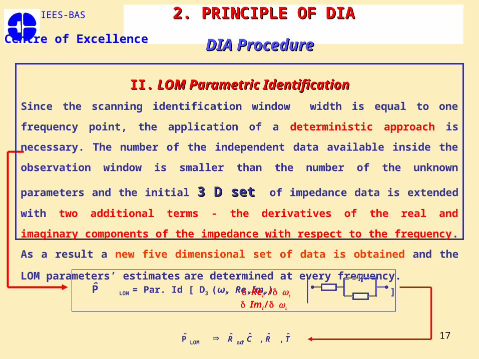
II.II. LOM Parametric IdentificationLOM Parametric Identification

Since the scanning identification window width is equal to one frequency point, the application

of a deterministic approach is necessary. The number of the independent data available inside

the observation window is smaller than the number of the unknown parameters and the initial 3 3

D setD set of impedance data is extended with two additional terms - the derivatives of the real and

imaginary components of the impedance with respect to the frequency.

As a result a new five dimensional set of data is obtained and the LOM parameters’ estimates

are determined at every frequency.

Rei / Imi/

IEES-BAS




T,R,C,RP adLOM

18

II.II. LOM Parametric Identification LOM Parametric Identification

IEES-BAS


Impedance of the LOMImpedance of the LOM

2. PRINCIPLE OF DIA - 2. PRINCIPLE OF DIA - DIA ProcedureDIA Procedure

]ˆlg,ˆlg,ˆlg,ˆlg,[lg CRRTDadest

New data set :New data set :

-Z''

/

Z' /

R

Rad

C

V is the vector of the parameters

2222ad1 ;

1)(i

T

RT

T

RR

V (2)

(1)2222ad1

i1

)(iT

RT

T

RRZ

)( ),( )(i effeff LRV (3)

)(d

)(d

d

)(d

d

)(d)(

eff

effeffeff

R

LRLT ˆ (4)

)(1

)()()(

22effad

T

RRR

ˆ

ˆˆ

(5)

)(2

] )(1 [

d

)(d)(

2

222eff

T

TRR

ˆ

ˆˆ

(6)

)()()( RTC ˆ/ˆˆ (7)

19

IIIIII

Frequency Analysis of the LOM Parameters

EstimatesLOM f ()P

Determines the model structure

IEES-BAS




III.III. Frequency analysisFrequency analysis of the LOM parameters’ estimates.of the LOM parameters’ estimates.

The analysis of the LOM parameters’ estimates frequency behaviour , which can be performed in different ways, provides for the structural and parametric identification of the impedance model. Every form of representation emphasizes specific parts of the model structure and thus their combination ensures a more complete and precise identification.

20

IEES-BAS





1. Temporal Analysis Temporal Analysis – direct recognition of lumped parameters

iL

)(] , , ,[ iiiiii νcr FˆˆˆˆL where the vector iL contains the decimal logarithms of the parameters :

ii Radlg ˆˆ ii Tˆ lg ii Rr ˆˆ lg ii Cc ˆˆ lg and;; ;; ;; )lg( 1 ii

For its further implementation the following notation will be used:

(9)

2lg )lg (lg f1

LOMT

i FFP

where Tf = 1/f and f is the frequencyAs far as Tf represents the time interval of perturbation, the function is a temporal

one and the corresponding analysis is termed temporal analysistemporal analysis..

(8)

The new experimentaldata set is:The new experimentaldata set is: ] , , , ,[5 iiiii cr ˆˆˆˆD (10)

21

IEES-BAS

Centre of Excellence2. PRINCIPLE OF DIA - 2. PRINCIPLE OF DIA - DIA ProcedureDIA Procedure


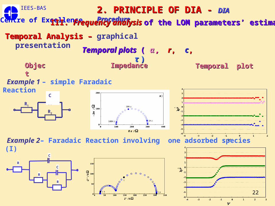
Temporal Analysis – Temporal Analysis – graphical presentation

The temporal analysis displays the functional dependencies of Eqn. (8). in two types of plots – temporal plottemporal plots s and spectral plotsspectral plots..

Temporal plotsTemporal plots

In the frequency regions, where the LOM corresponds to the object’s behaviour, i.e. to a sub-model with a structure of a time-constant (R and C in parallel connection – Example 1), the dependencies described by Eqn. 8 are frequency invariant and their temporal plots exhibit plateaus.

In Examples 2 - 4 the object is a Faradaic reaction involving one adsorbed species, i.e. the reaction has two steps and the observed plateaus are also two. They are separated by regions of frequency dispersion, which in this case correspond to the transition between the two reaction steps.

To summarize :To summarize : the presence of plateaus ensures the recognition of the model, while their position enables the parametric estimation.

22

IEES-BAS





Temporal plots Temporal plots ( ( αα , , rr, , cc, , ττ ))

R1

CPE

R2

C

0 100 200 300 4000

100

200a)

10Hz

100Hz 1Hz

- Im

/

Re /

ObjectObject ImpedanceImpedance Temporal plotTemporal plot

Example 1 – simple Faradaic Reaction

0 50 100 150 200 250 300 3500

50

100

150

1 k

1 -Z''

/ k

Z' / k

1 m

R

C

C

R

R

Example 2– Faradaic Reaction involving one adsorbed species (I)

23

R

C

C

R

R

Example 4– Faradaic Reaction involving one adsorbed species (III)

IEES-BAS





Temporal plots Temporal plots ( ( rr, , cc, , ττ ))

Example 3– Faradaic Reaction involving one adsorbed species (II)

ObjectObject ImpedanceImpedance Temporal plotTemporal plot

0 50 100 150 200 2500

50

100

1 k

1

-Z''

/ k

Z' / k1 m

R

C

C

R

R

24

IEES-BAS




The temporal analysis displays the functional dependencies of Eqn. (8). in two types of plots – temporal plottemporal plots s and spectral plotsspectral plots..

Spectral plotsSpectral plots

The Spectral presentation (analysis) offers an enhanced performance of the results obtained by the temporal analysis. It displays the dependencies of Eqn. 8 in the more informative spectral form Sj, which reveals the presence of a different number of time-constants:

where j denotes the corresponding parameter and S.T. symbolizes the spectral transformation procedure, which converts the plateaus of the temporal plots into spectral lines.

)](S.T.[ j,jj iyFS (11)

25

IEES-BAS




Spectral plotsSpectral plots

The simplest spectral transform can be regarded as a construction of an ordinary histogram. The parametric spectra are obtained by accumulating frequency bands with approximately equal values of the parameter . .

The intensity of the individual spectral peaks is estimated by introducing a dB grid, where an intensity of 10 dB corresponds to a frequency band of one decade. Since the spectral representation takes into account the frequency spacing of the real data, the amplitude of the spectral line is proportional to the length of the frequency interval where a given phenomenon is well pronounced.

To summarize :To summarize : The spectral presentation transforms the temporal plateaus into spectral peaks. The number of spectral lines gives the number of time-constants (R/C meshes) in the model.

The position of the spectral lines defines the value of the corresponding parameter.

) , , , ( jj ˆˆˆˆˆˆ rcyy

26

IEES-BAS



Spectral Transform Spectral Transform ( ( αα , , rr, , cc, , ττ ))

R

C

C

R

R

Example 2– Faradaic Reaction involving one adsorbed species (I)

R1

CPE

R2

C

ObjectObject Temporal plotTemporal plot Spectral plotSpectral plot

Example 1 – simple Faradaic Reaction

27

IEES-BAS



Spectral Transform Spectral Transform ( ( rr, , cc, , ττ ))

Example 4– Faradaic Reaction involving one adsorbed species (III)

6 3 0 -30

15

30

^C / F

In

ten

sity

/ d

B

^lgP

^R

2/

lg(-P)^

-3 0 3 6

^- C / F

^- R

2 /

c)

-4 -2 0 2 4 60

15

30

^T / s

Inte

nsi

ty /

dB

^lgP

d)

Example 3– Faradaic Reaction involving one adsorbed species (II)

R

C

C

R

R

Spectral plotSpectral plotObjectObject Temporal plotTemporal plot

28

IEES-BAS


Spectral Transform Spectral Transform – – Noise ImmunityNoise Immunity

The spectral transform plays the role of a consecutive integration, since the intensity of an individual spectral peak is proportional to the length of the frequency interval where the corresponding parameter’s estimate has close values. Thus the spectral transform provides for data stratification and for efficient filtration of non-statistical noise, because the presence of an outlier introduces only a fuzzy low intensity line, located away from the spectral kernel of the basic phenomenon .

Example on synthetic model of Faradaic Reaction involving one adsorbed species:

R

C1

C2

R1

R2

T1 = R1C1

T1 = R2C2

q = T2/T1 = 0.001

• Simulation of noise – by truncation;

• Simulation of non-Gaussian noise – by introduction of a “wild point” via 10% increase of Re.

29

IEES-BAS


Spectral Transform Spectral Transform – – Noise ImmunityNoise Immunity

Impedance diagramsImpedance diagrams q = T2/T1 = 0.001

0 3 60

3

a)

10 Hz

0.01 Hz

0.1 Hz

1 Hz

- Im

/ k

Re / k

7 digits

0 3 60

3

b)

0.01 Hz

0.1 Hz10 Hz

1 Hz

-Im

/ k

Re / k

Truncation to 4 digits

4 digits +wild point

0 3 60

3c)

10 Hz

0.01 Hz

0.1 Hz

1 Hz

-Im

/ k

Re / k

30

IEES-BAS


Spectral Transform Spectral Transform – – Noise ImmunityNoise Immunityq = T2/T1 = 0.001

4 digits +wild point7 digits Spectral PlotsSpectral Plots

• DIA recognizes the model with q = 0.001 (CNLS recognizes the model up to q = 0.01);

• DIA recognizes the model with q = 0.001 up to 4 digits. The procedure of truncation increases only the number of low intensity “fuzzy” lines in the vicinity of the 2 spectral peaks;

• The introduction of a “wild point” does not influence the selectivity of DIA, because its presence only gives additional “fuzzy line” located far away from the 2 basic peaks.

31

IEES-BAS


3. SECONDARY DIA -3. SECONDARY DIA - IntroductionIntroduction

When the LOM does not correspond to the object’s structure, frequency dependence is observed in the temporal plots. It may be due to:

R

C

C

R

R

• mixing of two neighbouring phenomena

• presence of frequency dispersion

(CPE, W etc).

or

0,0 0,1 0,2 0,3 0,40,0

0,1

0,2

1

-Z''

/

Z' /

1 m

CPE

The regions of mixing cannot produce

spectral peaks. They form ”tails” in the

spectral plots.

CPE

32

IEES-BAS


Although introduced to the identification of models with lumped elements, the applied LOM can be used for the recognition of frequency distribution.

This property increases the analytical power of the DIA since it ensures structural and parametric identification within a wider frequency range, including regions where the LOM does not correspond to the structure of the investigated object. Thus DIA can be applied for investigation of a wide variety of real samples, containing rough and inhomogeneous surfaces or inhomogeneous volume properties.

The identification of models with frequency dispersion behaviour is based

on the so-called Secondary Differential Impedance Analysis.Secondary Differential Impedance Analysis.

3. SECONDARY DIA -3. SECONDARY DIA - IntroductionIntroduction

33

IEES-BAS

Centre of Excellence 3. SECONDARY DIA 3. SECONDARY DIA

Differential Temporal AnalysisDifferential Temporal Analysis

)( αcrτ iiiii δ, δ, δ, δ, ν ˆˆˆˆD

The Secondary DIA is performed by differentiation of the logarithmic LOM parameters’ estimates with respect to the logarithm of the frequency. It presents their frequency dependence in the form:

where j denotes the corresponding LOM’s parameter estimate or .

Thus a new set of functions is obtained, which forms a new estimated data set :

Since the Secondary Analysis describes the differentiation of the temporal

functions, it is called Differential Temporal Analysis Differential Temporal Analysis.

)()d/ˆd(ˆjj, iii ΦL (12)

(13)

cr ˆˆˆ , ,

344 3 2 1 0 -1 -2 -3

-2

-1

0

1

2

3

P

^

IEES-BAS

Centre of Excellence3. SECONDARY DIA 3. SECONDARY DIA

Differential Temporal AnalysisDifferential Temporal Analysis

(14)

The derivatives of the parameters’ estimates become equal to 0 in the frequency range where the LOM corresponds to the nature of the impedance object, i.e for a model of a simple Faradaic reaction as well as for the plateaus of a lumped (homogeneous) model involving one or more adsorbed species

i j,

0αcrτ iiii ˆˆˆˆ

0 50 100 150 200 250 300 3500

50

100

150

200

250

300

350

1 k

1

-Z''

/ k

Z' / k

1 m

C1 C2

R2R1 R3

The two frequency bands, where is equal to 0 are separated by a bell-shaped region of transition, which corresponds to the mixing of the two time-constant type sub-models.

P

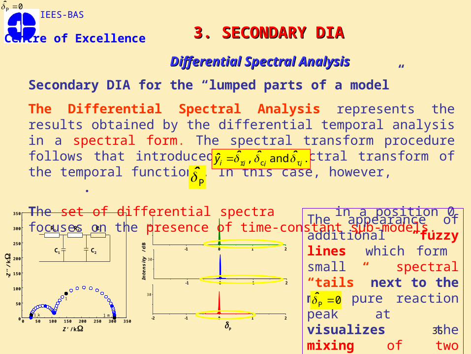
Secondary DIA for the “lumped parts of a model”

35

-2 -1 0 1 2

30

-1 0 1 2

30

-1 0 1 2

30

P

Inte

nsi

ty /

dB

^

IEES-BAS


Differential Spectral AnalysisDifferential Spectral Analysis

0 50 100 150 200 250 300 3500

50

100

150

200

250

300

350

1 k

1

-Z''

/ k

Z' / k

1 m

C1 C2

R2R1 R3

Secondary DIA for the “lumped parts of a model”

The Differential Spectral Analysis represents the results obtained by the differential temporal analysis in a spectral form. The spectral transform procedure follows that introduced in the spectral transform of the temporal functions. In this case, however, .

The set of differential spectra in a position 0 focuses on the presence of time-constant sub-models.

. and , τcr iiiiy ˆˆˆˆ

P

0P

The appearance of additional “fuzzy lines” which form small spectral “tails” next to the main pure reaction peak at visualizes the mixing of two uniform sub-models.

0P

36

IEES-BAS


Recognition of CPE DispersionRecognition of CPE Dispersion

0P

When the dispersion curve in the temporal plot has a constant slope, the -functions also acquire a constant value, different from 0, which is characteristic of this dispersion. In such cases the Secondary DIA is obligatory, since it can identify the dispersion zone in a more explicit way.

Temporal plotTemporal plot

The dispersion is described by straight lines, i.e. it has a constant slope.

n1CPE )(jA)(jZ

0,0 0,1 0,2 0,3 0,40,0

0,1

0,2

1

-Z''

/

Z' /

1 m CPE ImpedanceCPE Impedance(15)

The irregular electrode surface, due to surface roughness or non-uniformly distributed properties, leads to a dispersion of the parameters. Very often this behaviour is successfully approximated by an empirical relationship, known as constant phase element (CPE).

37

IEES-BAS


Recognition of CPE DispersionRecognition of CPE Dispersion

0P

The secondary frequency analysis in the case of CPE operates with the projection of the CPE impedance in the internal LOM’s space, represented in coordinates R, C and T:

lgR = r = - lg A + lg [cos(n/2)] – n lgω (16)

lgC = c = lgA – lg[sin(πn/2) – (1 – n)lgω (17)

lgτ = - lg – lg [tg (n/2) (18)

lgA = -lgR + lg[cos(n/2)] – n lg lg C + lg[(n/2)] + (1-n) lg (19)

The derivatives of equations (16) – (18) form a new set of a new set of interdependent interdependent

““δδ” ” functionsfunctions with definite for the CPE behaviourdefinite for the CPE behaviour, determined by the constant slope of the dispersion curves in the temporal plot:

ni r ni 1c 1crτ ii (20)

38

IEES-BAS


Example for Recognition of CPE DispersionExample for Recognition of CPE Dispersion

ni r ni 1c 1crτ ii

Differential Temporal Plot

c

Differential Spectral PlotThe combined differential spectral plot of , and , which is characterized by three distinct spectral peaks, can be regarded as a “fingerprint” of the CPE behaviour.

r cτ

0,3 0,7 1

39

IEES-BAS


TEST ExampleTEST Example: Find : Find the value of the CPE coefficient using the given Differential plots

(click on the correct value)

ni r ni 1c 1crτ ii


c

Differential Spectral Plot

-4 -3 -2 -1 0 1 2 3-1

0

1

2

P

^

The CPE coefficient is:

0 0.10 0.20

0.30 0.40 0.50

0.55 0.60 0.70

0.80 0.90 1

40

IEES-BAS


Recognition of Randles ModelRecognition of Randles Model

The application of the Secondary Differential Analysis promotes the capability of the DIA for model recognition. It can be applied to the identification of electrochemical elements or more complicated models with CPE in their structure. This section introduces some examples for the application of the DIA on synthetic models often used in electrochemical systems . Randles model (RND) is widely applied to electrochemical systems for modelling of a simple Faradaic reaction with a mass transport towards the electrode’s surface, limited by a linear semi-infinite diffusion.

C W

R2R1

The deviations from Fick’s law can be presented by modification of the Warburg impedance with CPE. The model is known as Modified Randles Model (MRND).

C BW

R2R1

CPE

41

The temporal analysis discovers three segments with differing frequency behaviour. The high frequency region I is frequency invariant. The low frequency parts II and III, however, show two types of frequency dispersion, which require a Secondary DIA.

The lack of frequency dispersion in segment I confirms the correspondence between the LOM and the object in this region, i.e. the recognized structure is a parallel connection between Rct (R) and Cdl (C).

IEES-BAS


Recognition of Randles ModelRecognition of Randles ModelDIA Results:DIA Results:

RND MRND

Temporal Analysis

The applied estimates data set is: ] , , , [ τcr iiii ˆˆˆD (21)

42

IEES-BAS



Temporal Analysis - Spectral presentation

The spectral plots sharply distinguish too types of behaviour – frequency independent, which is represented by a well defined spectral line, and frequency dependent, which forms a spectral “tail”. This result demonstrates the high sensitivity of the spectral analysis for the identification of time-constants.

The plateaus in the temporal plots and the spectral images ensure the parametric identification of the Rct/Cdl sub-model.

RNDMRND

43

IEES-BAS



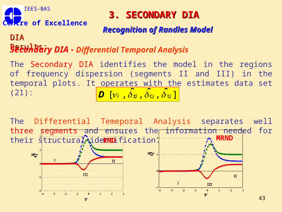
Secondary DIA - Differential Temporal Analysis

The Secondary DIA identifies the model in the regions of frequency dispersion (segments II and III) in the temporal plots. It operates with the estimates data set (21):

The Differential Temeporal Analysis separates well three segments and ensures the information needed for their structural identification.

] , , , [ τcr iiii ˆˆˆD

RND MRND

44

IEES-BAS



Secondary DIA - Differential Temporal Analysis

Segment I: Segment I: The dependencies obtained for segment I confirm the structure of resistance and capacitance in parallel, since 0 τcr iii ˆˆˆ

Segment IISegment II

For RND the obtained dependencies recognize Warburg Impedance, since

0.5 r ni 0.51c ni 1crτ iii ˆˆˆ

For MRND the obtained dependencies recognize CPE (n = 0.4), since

0.4 r ni 0.61c ni 1crτ iii ˆˆˆ

Segment III: Segment III: The bell-shaped region III defines the region of mixing between the two sub-models in the Randles structure.

45

IEES-BAS



Secondary DIA - Differential Spectral Analysis

The combined Differential Spectral Plot ( see page 46)( see page 46) represents in an explicit way the structural and parametric identification, emphasizing the two kernels of that structure .

The spectral lines in zero position (segment I) manifest the presence of the time-constant sub-model, corresponding to the Faradaic reaction.

The combination of the other three spectral peaks (segment II) visualizes the transport limitation:

• For values 0.5, 0.5 and 1 - Warburg impedance (RND);

•For values 0.3, 0.7, 1 - CPE (MRND).

46

IEES-BAS



Secondary DIA - Differential Spectral Analysis

C BW

R2R1

CPE

C W

R2R1

47

IEES-BAS


Recognition of Simple Faradaic Reaction with Capacitive CPE Recognition of Simple Faradaic Reaction with Capacitive CPE

The impedance diagram of a modified time-constant model with a capacitive CPE is characterized by depressed semicircle, which is often observed in real systems.

In electrochemical systems this structure is known as modified polarizable electrode.

0 200 400 6000

200

400

600

1 kHz

1 Hz

-Z''

/

Z' / 1 mHz

R1

CPE R2

48

IEES-BAS



DIA Results:DIA Results:

Temporal plot

Temporal Analysis

The applied estimates data set is:

The behaviour of the temporal plots is surprising to some extent, since the dispersion concerns not only c and τ, but also r within the whole frequency range. Formally the temporal plots can be divided into a high frequency segment I and a low frequency segment II .


49

IEES-BAS



DIA Results:DIA Results:

Temporal Analysis

In the r – temporal plot the two segments (I and II) can be regarded as separated by a region of pseudo-mixing (segment III), which has a shape close to a plateau and creates the small intensity spectral peak in the spectral plots. It also determines the approximation to the estimate of the model’s resistance R (Rct), i.e. the temporal analysis of segment III in the temporal plot ensures its parametric identification.

Temporal plot Spectral plot

50

IEES-BAS



Secondary DIA

The Secondary DIA identifies the model in the frequency dispersion regions (segments I and II) in the temporal plots. It operates with the estimates data set (21):


The Differential Temeporal Analysis of Segment I Segment I distinguishes dependencies of CPE-type, which ensure identification of the CPE exponent n (n = 0.8).

Knowing n, the parameter A can be also calculated.

0.8 r ni 0.21c ni 1crτ iii ˆˆˆ (22)

Differential Temporal Plot Differential Spectral Plot

51

IEES-BAS



Secondary DIA

The Differential Temeporal Analysis of Segment I performs the parametric identification, since it recognizes the CPE exponent n.

The Differential Temporal Analysis of Segment IISegment II, however, ensures the structural identification of the model, since the results, obtained for are characteristic only for this model:

] , , [ iii cr ˆˆ

0.8 r ni 1.81c ni 1crτ iii ˆˆˆ (23)


52

IEES-BAS



Secondary DIA

The Structural and Parametric Identification of a Faradaic Reaction with Capacitive CPE is ensured by simultaneous Secondary DIA of both segments I and II from the temporal plots, following the correlated dependencies (22) and (23). The illustrative Differential Spectral Plot can be regarded as a “fingerprint” of the model.


53

-2 -1 0 1 2

-1 0 1 2

-1 0 1 2

30

P

Inte

nsi

ty /

dB

^

-2 -1 0 1 2

-1 0 1 2

-1 0 1 2

30

P

Inte

nsi

ty /

dB

^

0 200 400 6000

200

1 k

1

-Z''

/

Z' / 1 m

Model AModel A

0 50 100 150 200 2500

50

100

1 k

1

-Z''

/ k

Z' / k1 m

Model BModel B

or orR1

CPE R2

Circuit 2

C1 C2

R2R1 R3

Circuit 1

C1 C2

R2R1 R3

Circuit 1

Recognize the model using the Differential Temporal PlotsRecognize the model using the Differential Temporal Plots

R1

CPE R2

Circuit 2

IEES - BAS

Centre of Excellence TEST:TEST:

54

VERY HIGH:VERY HIGH:

SelectivitySelectivity Noise immunityNoise immunity RobustnessRobustness

NO NEEDof a preliminary

working Hypothesis(the model is

extracted from the data)

MAIN ADVANTAGES of DIA:MAIN ADVANTAGES of DIA:

DISTRIBUTIONRecognition

&Characterization





&Characterization




VERY HIGH:

Selectivity Noise immunity Robustness

VERY HIGH:

Selectivity Noise immunity Robustness


&Characterization

IEES-BAS


53

IEES - BAS

Centre of Excellence4. DIA APPLICATION of YSZ 4. DIA APPLICATION of YSZ

Solid ElectrolyteSolid Electrolyte

high conductivityYSZ

Oxygen separators

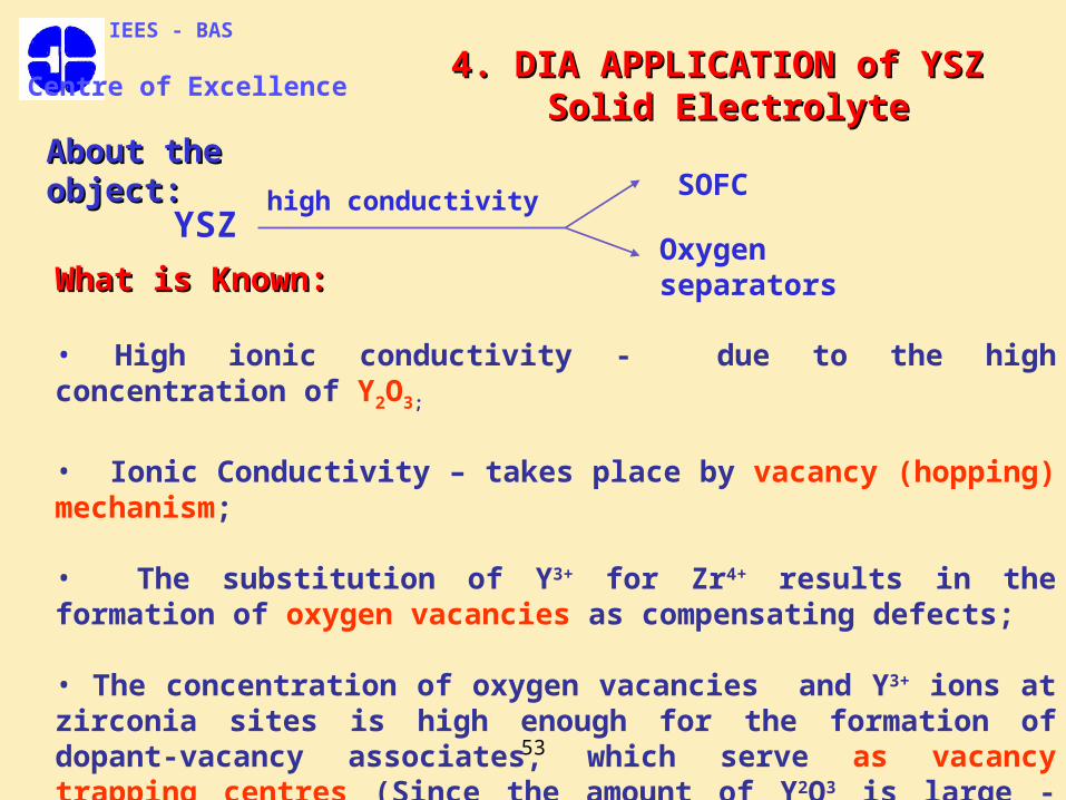
SOFCAbout the object:About the object:

What is Known:What is Known:

• High ionic conductivity - due to the high concentration of Y2O3;

• Ionic Conductivity – takes place by vacancy (hopping) mechanism;

• The substitution of Y3+ for Zr4+ results in the formation of oxygen vacancies as compensating defects;

• The concentration of oxygen vacancies and Y3+ ions at zirconia sites is high enough for the formation of dopant-vacancy associates, which serve as vacancy trapping centres (Since the amount of Y2O3 is large - about 9 wt%):

(Y’(Y’Zr Zr VV....OO))-- (mainly) + + (Y’(Y’Zr Zr VV....

OO))x x (less)

56

What is Uncertain and Unknown:What is Uncertain and Unknown:

1. Conductivity:• The temperature dependence of mobility and concentration of “free”

vacancies able to take part in the transport process; • Possible changes of the activation energy Ea with the temperature?• Possibility for formation of vacancy ordered micro-domain structures due to

the high concentration of the acceptors and thus to possibility for complex defect interactions.

2. Surface oxygen exchange: The current trends for reduction of SOFC operating temperature below 1000oC concern not only the increase of the electrolyte conductivity and the electrodes catalytic activity, but also the surface oxygen exchange, which may become the rate limiting step in the oxygen transfer process.

IEES - BAS

Centre of Excellence4. DIA of YSZ 4. DIA of YSZ

57

IEES - BAS


Advantages of the DIA Studies :

The application of techniques for common investigation of both the oxygen exchange and ionic conductivity of the bulk oxide will provide for better re-evaluation of YSZ transport properties.

• One possibility is the application of isotope exchange and secondary ion mass spectrometry (SIMS). The small number of publications is due to the difficulties in performing tracer experiments on solid electrolytes;

• EIS can investigate both the ionic conductivity and oxygen surface exchange, since it ensures clear distinction between the bulk and grain boundary resistance and the electrode reaction.

•The application of DIA eliminates the need of preliminary hypotheses for the description of the complicated electrode reaction, which should be divided into individual steps, involving charge transfer across the interface, as well as non-charge transfer processes such as adsorption, solid state diffusion, gas phase diffusion etc.

58

YSZ

Single crystal (9.5 mol % Y2O3)

Polycrystalline (8.5 mol % Y2O3)

Electrodes: (Platinum)

Instrument • Solartron FRA 1260

Experimental: Experimental:

Conditions: • Amplitude = 50 mV;•Frequency range: 13 MHz - 0,1 Hz;•density: 9 points/decade;•temperatures: room to 1000o C •parasitic inductance elimination

IEES - BAS


59

Experimental: Experimental:

IEES - BAS


Impedance diagrams of YSZ single crystal:• frequency range: 13 MHz – 0.1 Hz;• temperature interval: room – 1000o C;• data after L-correction.

60

T < 500°CT > 500°C

IEES - BAS


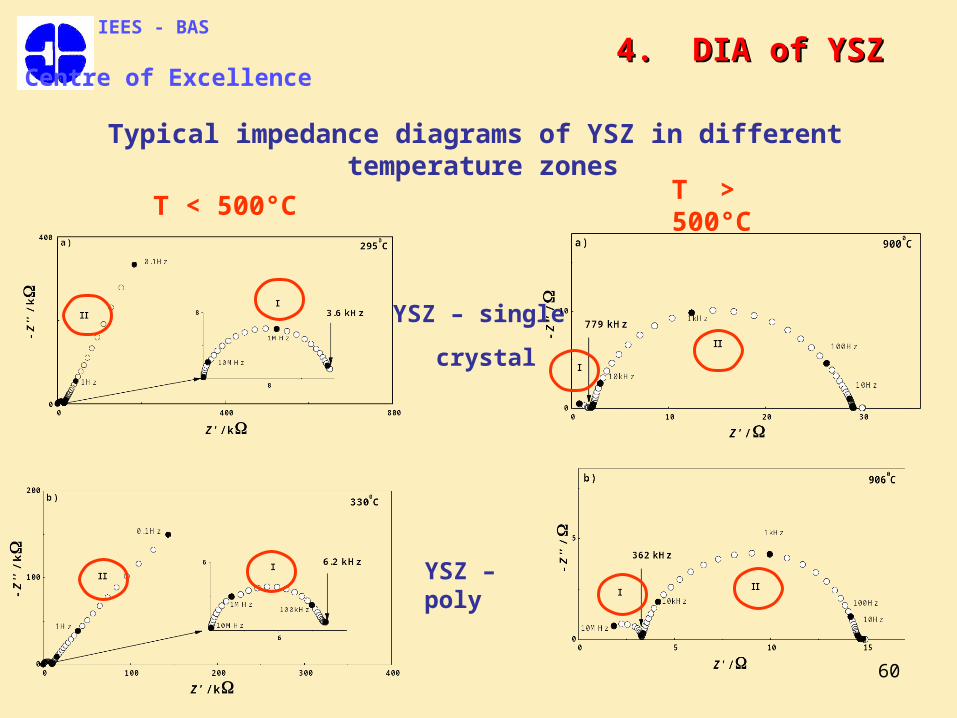
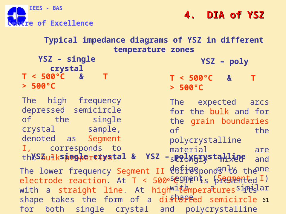
Typical impedance diagrams of YSZ in different temperature zones

YSZ – poly

YSZ – single

crystal

61

IEES - BAS


Typical impedance diagrams of YSZ in different temperature zones

T < 500°C & T > 500°C

The high frequency depressed semicircle of the single crystal sample, denoted as Segment I, corresponds to the bulk properties.

YSZ – single crystal YSZ – poly

T < 500°C & T > 500°C

The expected arcs for the bulk and for the grain boundaries of the polycrystalline material are strongly mixed and define only one segment (Segment I) with a similar shape.

YSZ – single crystal & YSZ – polycrystalline

The lower frequency Segment II corresponds to the electrode reaction. At T < 500o C it is presented with a straight line. At high temperatures its shape takes the form of a distorted semicircle for both single crystal and polycrystalline sample.

62

IEES - BAS


General RemarksGeneral Remarks

The examples based on single crystal and polycrystalline samples of YSZ demonstrate the effect of the combined application of the temporal and the differential temporal analyses to the complete identification of the corresponding models.

For DIA investigation of both the electrode and the reaction (oxygen exchange) conductivities, which have response in different frequency regions, precise frequency segmentation is performed in the R - temporal plot.

In this study the R -temporal plot is mainly used since it is the basis for parametric identification of the resistance, which ensures quantitative characterization of the phenomena under investigation.

63

Temporal plotTemporal plot

There are two well distinguished regions with different temporal behavior.

IEES - BAS


YSZ Single Crystal : YSZ Single Crystal : rr-- Temporal plot segmentation Temporal plot segmentation

The low frequency Segment II Segment II is frequency dependent and a Secondary DIA has to be performed for its identification.

The high frequency Segment ISegment I forms a plateau, i.e. it is frequency independent and determines the bulk resistance of the single crystal.

rr

ττcc

Spectral plot of Spectral plot of Segment ISegment I

The rr, cc and ττ spectral images give a single spectrum, which confirms the time-constant model, i.e. a parallel connection of resistance and capacitance.

R

C

64

Segment I combines two regions – IA and IB. Both of them are frequency invariant and thus they recognize the characteristic for this system two time-constant model with Voigt’s structure, applied to solid state. Sub-segment I A determines the bulk resistance Rb and sub-segment I B - the grain boundary resistance Rgb.

IEES - BAS


YSZ Polycrystalline : YSZ Polycrystalline : rr-- Temporal plot segmentation Temporal plot segmentation

The low frequency Segment II is frequency dependent and a Secondary DIA has to be performed for its identification.

The two spectral lines in the rr, cc and ττ spectral plots confirm the identification of a two time-constant model.

R

C

R

C

65

IEES - BAS

Centre of Excellence4. DIA ON YSZ 4. DIA ON YSZ

YSZ Single Crystal : YSZ Single Crystal : Secondary DIA Secondary DIA (below 500(below 500ooC)C)

The investigation of the electrode reaction concerns the analysis of Segment II, which requires Secondary DIA for both the single crystal and the polycrystalline samples. Since the approach is the same and the results are similar, only the example with the single crystal sample is included.

The Secondary DIA of Segment II at temperatures below 500o C shows, that the parameters , and obey the mutual relationships (20), which identify CPE of Warburg type, since the values of n vary in the interval between 0.5 and 0.6 for that temperature range.

Temporal plot ofTemporal plot of rr Differential Spectral PlotDifferential Spectral Plot

r c

-1 0 1 20

30

P

^

b)

0 1 20

30

Inte

nsi

ty /

dB

0 1 20

30

295 0 C

66

IEES - BAS


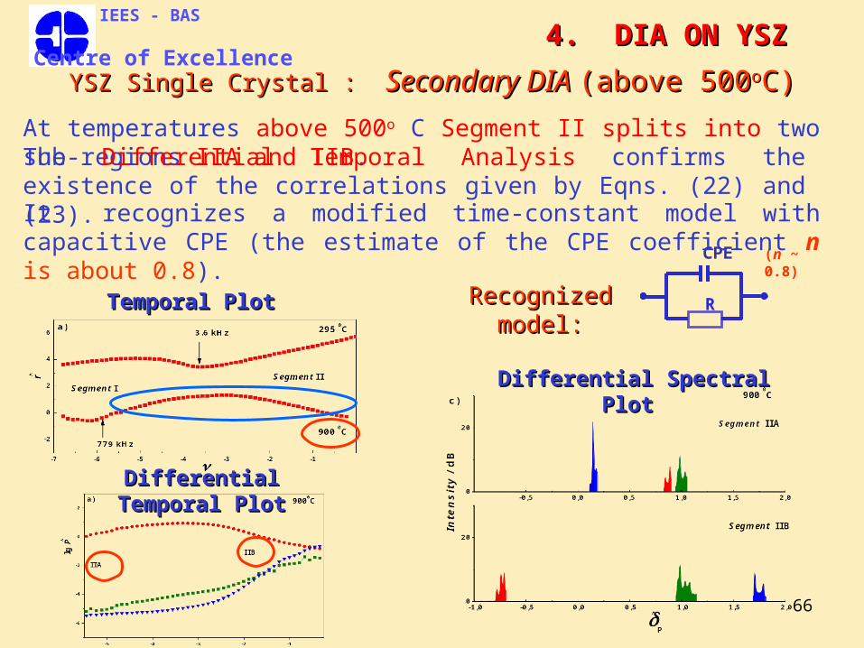
YSZ Single Crystal : YSZ Single Crystal : Secondary DIA Secondary DIA (above 500(above 500ooC)C)

At temperatures above 500o C Segment II splits into two sub-regions IIA and IIB.

Temporal PlotTemporal Plot R

CPE (n ~ 0.8)

Recognized model:Recognized model:

It recognizes a modified time-constant model with capacitive CPE (the estimate of the CPE coefficient n is about 0.8).

Differential Temporal PlotDifferential Temporal Plot

Differential Spectral Plot Differential Spectral Plot

The Differential Temporal Analysis confirms the existence of the correlations given by Eqns. (22) and (23).

67

Arrhenius Plots and Activation Energy EArrhenius Plots and Activation Energy Eaa (bulk and grain boundary)(bulk and grain boundary)

YSZ – single crystalYSZ – single crystal

5

6

lg

1000 / K

Ea = 1,14 eV;

(bulk)

0,5 1,0 1,5 2,0 2,5

0

1

2

3

4

7

T-1

0,5 1,0 1,5 2,0

0

1

2

3

4

5

6

lg

1000T -1/ K

Ea = 1.10; 0.31 eV (g.b)

Ea = 1.13; 0.29 eV (bulk)

YSZ – polycrystallineYSZ – polycrystalline

IEES - BAS


The parametric identification of the resistivity corresponding to the bulk, to the grain boundaries and to the electrode reaction processes ensures the building of the Arrhenius plots and thus the calculation of their activation energies Ea.

The Arrhenius plots for both the single crystal and the polycrystalline sample are characterized with a well pronounced kink in the range about 650oC. The activation energies Ea of the bulk and the grain boundaries are smaller at higher temperatures.

68

Arrhenius plots and calculation of EaArrhenius plots and calculation of Ea(for the bulk and electrode reaction of single crystal)(for the bulk and electrode reaction of single crystal)

0,5 1,0 1,5 2,0 2,5

0

1

2

3

4

5

6

7

lg

1000T -1/ K

Ea = 1,12; 0,66 eV

reaction

YSZ bulk

IEES - BAS


There is a kink in the Arrhenius plot of the electrode reaction. It marks a change in the activation energy from 0.66 eV at temperatures below 650oC to 1,21 eV at temperatures above 650oC.

The observed changes of the activation energy of the bulk conductivity and the oxygen exchange reaction at one and the same temperature (650oC) are an evidence for the correlation between the bulk and surface properties.

69

IEES


The technique of the DIA was developed for improvement of the model identification, eliminating the subjective step of an a priori selected hypothetical model(s) (the weak point in the classical (parametric) identification).

Thus it is expected, that the combination of the two procedures would increase the analytical power and information capability of the Electrochemical Impedance Spectroscopy.

70

IEES


It is my pleasure to It is my pleasure to Acknowledge with gratitude:Acknowledge with gratitude:

• EC – EESD - Part B: Energy Program (project NNE5/2002/18) and

• The ROYAL SOCIETYfor the financial support;

• UNESCO – UVO ROISTE and EICIS for the professional discussions environment;

• MY COLLEAGUES:Zdravko Stoynov, who invented and advances the

DIA technique, Geri Raikova from IEES,John Kilner and Stephen Skinner from Imperial

College – London

for the wonderful partnership and fruitful collaboration.

71

Journal of Electroanalytical Chemistry Vol. 572, 2004, pp 377-387

SECONDARY DIFFERENTIAL IMPEDANCE ANALVSIS – A TOOL FOR RECOGNITION OF CPE BEHAVIOR

D. Vladikova, Z. Stoynov

Central Laboratory of Electrochemical Power Sources, Bulgarian Academy of Sciences

AbstractThe procedure of a secondary DIA, which analyses the frequency dependence of the local operating model parameters’ estimates in the zones where there is no adequacy between the object and the local estimator. The new algorithm is successfully examined on synthetic models of CPE, Warburg, Randles, Randles with CPE modification, simple Faradaic reaction with CPE capacitance, as well as on real data obtained on yttrium iron garnet single crystals and yttria stabilized zirconia single crystals.

Keywords: ac impedance; Conductivity; Diffusion; CPE; Differential impedance analysis; Model recognition

72

Journal of the European Ceramic Society Vol. 24, 2004, pp 1121-1127

APPLICATION OF THE DIFFERENTIAL IMPEDANCE ANALYSIS FOR INVESTIGATION OF ELECTROCERAMICS

D. Vladikova1, Z. Stoynov1, M. Viviani2

1Central Laboratory of Electrochemical Power Sources, Bulgarian Academy of Sciences 2National Research Council, Institute for Energetics and Interphases, Genoa Department

AbstractThis work shows the enhanced performance of Impedance Spectroscopy for investigation and characterization of electroceramics by applying a new structural approach for data analysis, called Differential Impedance Analysis (DIA). The main advantage of this technique is the possibility for model identification directly from the experimental data, i.e. without the use of a preliminary working hypothesis. DIA provides for separation and phenomenological characterization of the different steps involved in the investigated object. The capabilities of the method are demonstrated in conductivity studies of yttrium iron garnet (YIG) single crystal and Er doped PTCR BaTiO3. The analysis ensures a more detailed investigation of the bulk properties of YIG, including the separation and characterization of the hopping conductivity. The application of DIA on BaTiO3 enriches the information about the role of the ferroelectric domain structure on the PTCR.

Keywords: BaTiO3 and titanates; Differential impedance analysis; Electrical conductivity; Ferrites; Ferroelectric properties

73

Bulgarian Chemical Communications, Volume 36, Number 1, 2004, pp 29-40

CONDUCTIVITY STUDIES OF SOLID OXIDE MATERIALS FOR ELECTRICAL APPLICATIONS

D. Vladikova

Institute of Electrochemistry and Energy Systems, Bulgarian Academy of Sciences

AbstractConductivity studies of solid oxide electroceramics. The method can distinguish between the bulk and the grain boundary contributions, as well as the electrode reaction. Both advantages and problems are discussed. In addition some recent improvements of the impedance data analysis, based on the technique of the Differential Impedance Analysis, are presented. They are illustrated with examples of conductivity studies on yttrium iron garnet single crystal with ferrimagnetic properties and Er doped barium titanate with positive temperature coefficient of the resistivity.

Key words: conductivity, electroceramics, impedance spectroscopy, yttrium iron garnet, Er doped barium Key words:

74

Bulgarian Chemical Communications, Volume 36, Number 1, 2004, pp 66-71

DIFFERENTIAL IMPEDANCE ANALYSIS OF BOUNDED CONSTANT PHASE ELEMENT

G. Raikova, D. Vladikova, Z. Stoynov

Institute of Electrochemistry and Energy Systems, Bulgarian Academy of Sciences

AbstractThe technique of the Differential Impedance Analysis (DIA) is applied for the identification of the so called bounded constant phase element (BCP), which describes the impedance of a bounded homogeneous layer with finite thickness and conductivity following constant phase element (CPE) behaviour. The enhanced identification capability of DIA is approbated on two models – a BCP one and a model of a simple Faradaic reaction with similar shapes of the impedance diagrams, presented with part of a semi-circle. DIA ensures a clear distinction between the two models.

Key words: Electrochemical Impedance Spectroscopy, Constant Phase Element, Bounded Constant Phase Element, Differential Impedance Analysis

75

Electrochimica Acta Vol. 47, pp2943-2951, 2002

SELECTIVITY STUDY OF THE DIFFERENTIAL IMPEDANCE ANALYSIS - COMPARISON WITH THE COMPLEX NON-LINEAR

LEAST-SQUARES METHOD D. Vladikovaa, P. Zoltowskib, E. Makowskab, Z. Stoynova

aCentral Laboratory of Electrochemical Power Sources, Bulgarian Academy of Sciences bInstitute of Physical Chemistry, Polish Academy of SciencesAbstract

The analytical power of the differential impedance analysis (DIA) as a new approach for model identification is investigated. The minimum of the ratio q of the two time-constants T1and T2 (q = T2/T1) describing a two step reaction with ladder structure, at which the second time-constant T2 is recognized, is accepted as a measure for the selectivity evaluation. The investigation is performed on synthetic models with variation of q in the interval from 30 to 0.001. The influence of data quality is studied by applying data truncation from seven to two digits, as well as by introduction of a wild point. Experimental data measured on two actual dummy cells with q equal to 30 and 0.03, respectively, are also analyzed. The results are compared with those obtained by applying the algorithm of the wide-spread complex non-linear least-squares method, performed on Zview software product. The comparative study demonstrates a higher selectivity of the DIA, combined with an additional noise immunity and increased robustness of the analysis.

Keywords: Electrochemical impedance spectroscopy; Differential impedance analysis; Complex non-linear least-squares; System identification; Selectivity

76

15ème Forum sur les Impedances Electrochimiques, 9 décembre 2002, Paris, France, pp 3-14

DIFFERENTIAL IMPEDANCE ANALYSIS – PRINCIPLE AND APPLICATION

Z. Stoynov


AbstractThe development of the modern instrumentation for Impedance Spectroscopy has led to its intensive application for investigation of large variety of practical objects. The classical identification of appropriate models for those objects meets strong limitations caused by the lack of theoretical developments as well as by the fuzzy nature of the studied processes. The aim of the Differential Impedance Analysis is the overcome these limitations and to serve as powerful analytical tool for investigation of unknown objects or objects with distributed parameters.

Key words: Impedance Spectroscopy, Differential Analysis, Fuzzy Modeling, Spectral Transform.

77

15ème Forum sur les Impedances Electrochimiques, 9 décembre 2002, Paris, France, pp 3-14

ANALYSE SPECTRALE D'IMPÉDANCE DIFFÉRENTTIELLE DES MODÈLESCINTÉTIQUES FOUNDAMENTAUX

Z. Stoynov1, H. Takenouti2, M. Keddam2, D. Vladikova1, G. Raikova1

1Central Laboratory of Electrochemical Power Sources, Bulgarian Academy of Sciences 2UPR15 du CNRS, Physique des Liauides et Electrochimie,

Universite Pierre et Marie Curie AbstractL’Analyse d’impédance différentielle (DIA) est appliquée pour les différents modèles cinétiques fondamentaux afin d’établir reconnaissance de modèle mécanistique par une nouvelle approche structurale. La comparaison des résultats expérimentaux et la structure prédéfinie permettra alors de déterminer sans hypothèse préliminaire, le mécanisme réactionnel adéquat. Les modèles de bases utilisent les schémas électriques équivalents déduits de réaction électrochimique; comme exemple, le transfert de charge en une seule étape et ceux impliquant une ou deux espèces intermédiaires de réaction. Nous illustrerons notamment dans le cas où la constante de temps de relaxation d’espèce intermédiaire est proche de celle définie par la capacité de double couche et la résistance de transfer! De charge. Nous présenterons également comment le modèle avec une capacité en parallèle avec une resistance permet d’appréhender l’impédance faradique sous forme inductive.

78

Materials for Lithium-Ion Batterie, Eds. C. Julien and Z. Stoynov NATO Science Series 3. High Technology –Vol. 85

Kluwer Academic Publishers pp 371-380, 2000

ADVANCED IMPEDANCE TECHNIQUES FOR LITHIUM BATTERIES STUDY

Part IV: Differential Impedance Analysis Z. Stoynov


AbstractThe aim of the experimental analysis is the interpretation of impedance data. It can follow two different pathways: the confirmation of a preliminary stated hypothetical model, or alternatively the derivation of the working model from the experimental result itself. The method of frequency scanning analysis based on a moving point to point estimator is summarized. The essentials of the local differential analysis are presented. The important properties of this new method are discussed.

79

Polish J. Chem., Vol. 71, 1997, pp1204-1210

DIFFERENTIAL IMPEDANCE ANALYSIS – AN INSIGHT INTO THE EXPERIMENTAL DATA

Z. Stoynov


AbstractA new method for analysis of the experimental data of the impedance spectroscopy is presented. The method is based on the assumption of a local operating model. Using the derivatives of the impedance with respect to frequency, the model parameters and their effective time-constants are calculated for each frequency. The analytical equations are used as a moving estimator over the entire frequency range. Important properties of the studied system can be derived.

Key words: impedance analysis, impedance spectroscopy, splines

80

Electrochimica Acta Vol. 35, No. 10, 1990,pp1493-1499

IMPEDANCE MODELLING AND DATA PROCESSING: STRUCTURAL AND PARAMFTRICAL ESTIMATION

Z. Stoynov


AbstractIdentification of the appropriate model is the aim of experimental data analysis. Some principal problems of the classical approach for parametrical identification are discussed. A new method for structural identification where the working model is derived from the experimental results is developed. Some recent results which expand the applicability of the method arc also given.

Key words: electrochemical impedance, identification, structural spectroscopy.

81

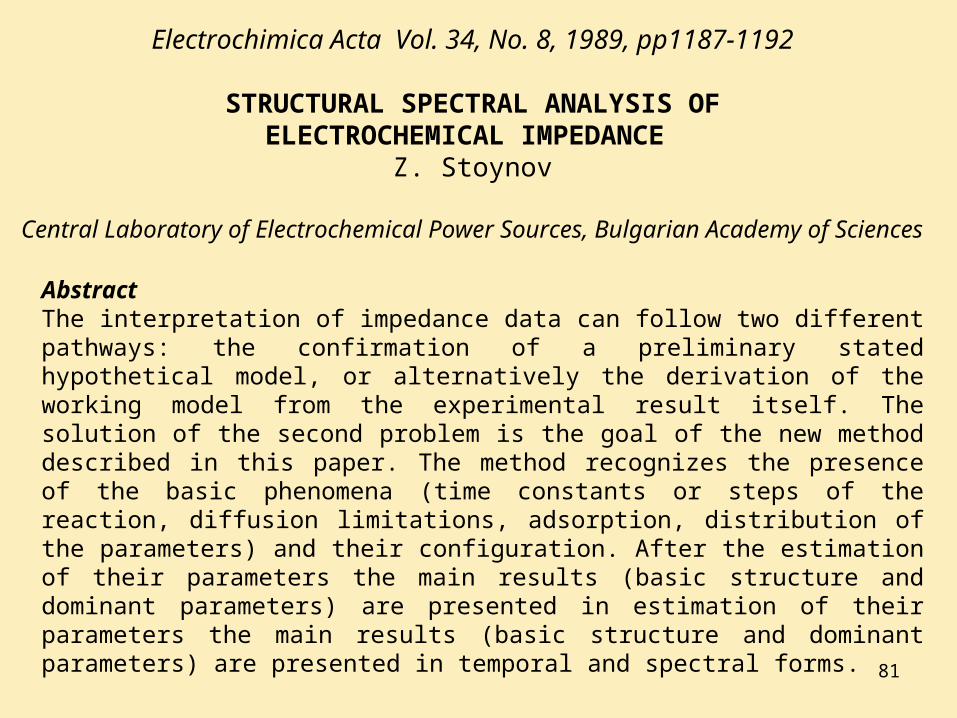
Electrochimica Acta Vol. 34, No. 8, 1989, pp1187-1192

STRUCTURAL SPECTRAL ANALYSIS OFELECTROCHEMICAL IMPEDANCE

Z. Stoynov


AbstractThe interpretation of impedance data can follow two different pathways: the confirmation of a preliminary stated hypothetical model, or alternatively the derivation of the working model from the experimental result itself. The solution of the second problem is the goal of the new method described in this paper. The method recognizes the presence of the basic phenomena (time constants or steps of the reaction, diffusion limitations, adsorption, distribution of the parameters) and their configuration. After the estimation of their parameters the main results (basic structure and dominant parameters) are presented in estimation of their parameters the main results (basic structure and dominant parameters) are presented in temporal and spectral forms.

82

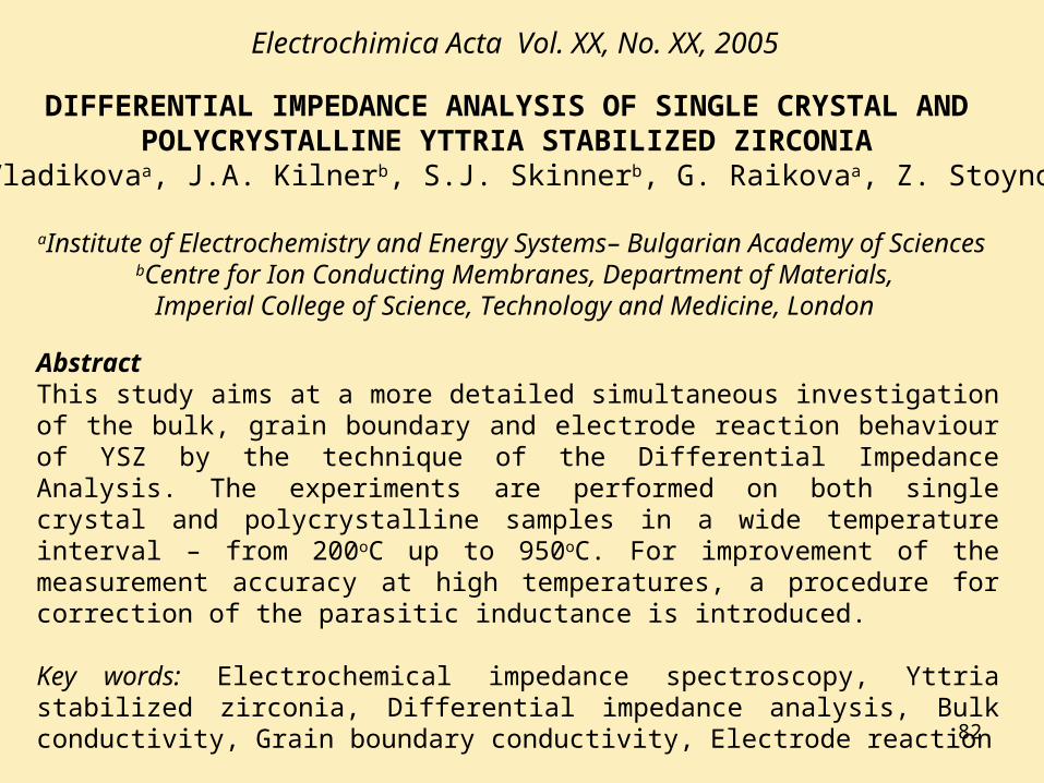
Electrochimica Acta Vol. XX, No. XX, 2005

DIFFERENTIAL IMPEDANCE ANALYSIS OF SINGLE CRYSTAL AND POLYCRYSTALLINE YTTRIA STABILIZED ZIRCONIA

D. Vladikovaa, J.A. Kilnerb, S.J. Skinnerb, G. Raikovaa, Z. Stoynova

aInstitute of Electrochemistry and Energy Systems– Bulgarian Academy of Sciences bCentre for Ion Conducting Membranes, Department of Materials,Imperial College of Science, Technology and Medicine, London

AbstractThis study aims at a more detailed simultaneous investigation of the bulk, grain boundary and electrode reaction behaviour of YSZ by the technique of the Differential Impedance Analysis. The experiments are performed on both single crystal and polycrystalline samples in a wide temperature interval – from 200oC up to 950oC. For improvement of the measurement accuracy at high temperatures, a procedure for correction of the parasitic inductance is introduced. Key words: Electrochemical impedance spectroscopy, Yttria stabilized zirconia, Differential impedance analysis, Bulk conductivity, Grain boundary conductivity, Electrode reaction

83

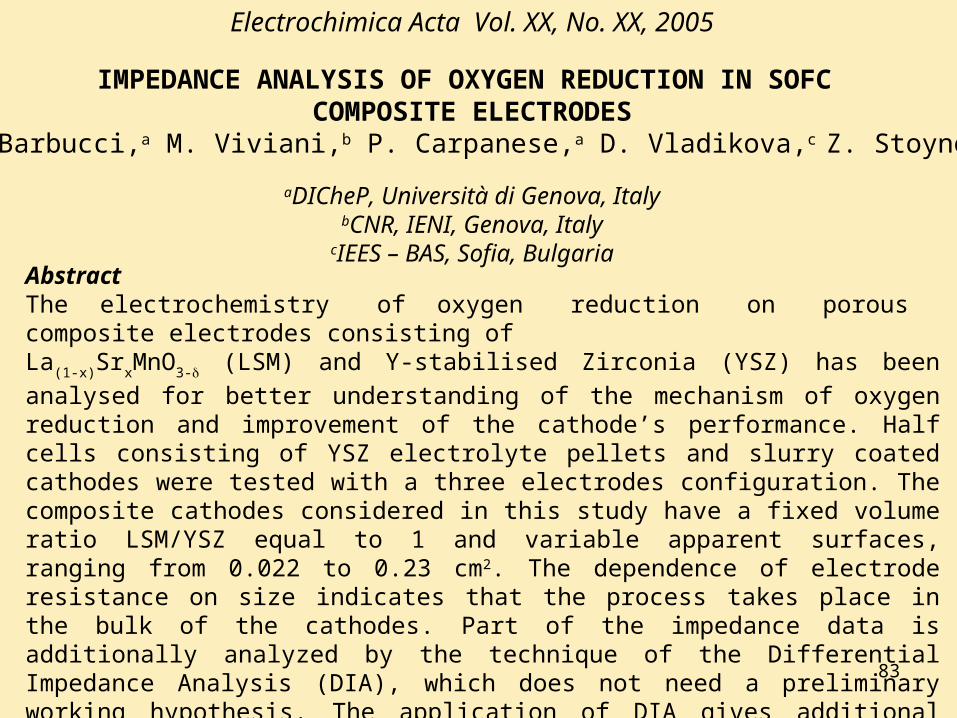
Electrochimica Acta Vol. XX, No. XX, 2005

IMPEDANCE ANALYSIS OF OXYGEN REDUCTION IN SOFC COMPOSITE ELECTRODES

A. Barbucci,a M. Viviani,b P. Carpanese,a D. Vladikova,c Z. Stoynovc

aDICheP, Università di Genova, ItalybCNR, IENI, Genova, Italy

cIEES – BAS, Sofia, BulgariaAbstractThe electrochemistry of oxygen reduction on porous composite electrodes consisting of La(1-x)SrxMnO3- (LSM) and Y-stabilised Zirconia (YSZ) has been analysed for better

understanding of the mechanism of oxygen reduction and improvement of the cathode’s performance. Half cells consisting of YSZ electrolyte pellets and slurry coated cathodes were tested with a three electrodes configuration. The composite cathodes considered in this study have a fixed volume ratio LSM/YSZ equal to 1 and variable apparent surfaces, ranging from 0.022 to 0.23 cm2. The dependence of electrode resistance on size indicates that the process takes place in the bulk of the cathodes. Part of the impedance data is additionally analyzed by the technique of the Differential Impedance Analysis (DIA), which does not need a preliminary working hypothesis. The application of DIA gives additional information about the dominant phenomena, based on comparative study of the cathode behaviour of LSM and the composite materials. Key words: Electrochemical impedance spectroscopy, Solid oxide fuel cells, LSM/YSZ Composite cathode materials, Differential impedance analysis

84

IEES-BAS


TEST Example TEST Example :: Find Find the value of the CPE coefficient using the given Differential plots.

ni r ni 1c 1crτ ii


c


-4 -3 -2 -1 0 1 2 3-1

0

1

2

P

^

The value is not correct!

NONO

85

IEES-BAS


TEST ExampleTEST Example: : Find Find the value of the CPE coefficient using the given Differential plots

ni r ni 1c 1crτ ii


c


-4 -3 -2 -1 0 1 2 3-1

0

1

2

P

^

The value is correct!

You have recognized Warburg ImpedanceWarburg Impedance,

since n = (1 – n) = 0.50.5

0,5 0,5 1

Warburg

86

0 50 100 150 200 2500

50

100

1 k

1

-Z''

/ k

Z' / k1 m

0 200 400 6000

200

1 k

1

-Z''

/

Z' / 1 m

Model AModel A Model BModel B

R1

CPE R2

C1 C2

R2R1 R3

Circuit 1Circuit 1Circuit 2Circuit 2

Y E S !Y E S !

IEES - BAS


87

0 50 100 150 200 2500

50

100

1 k

1

-Z''

/ k

Z' / k1 m

0 200 400 6000

200

1 k

1

-Z''

/

Z' / 1 m

Model A Model A Circuit 1Circuit 1

R1

CPE R2

C1 C2

R2R1 R3

Model BModel B Circuit 2Circuit 2

N O !!!N O !!!

IEES - BAS


1 iees - bas centre of excellence d. vladikova, institute of electrochemistry and energy systems,...

Documents