1

Huawei Report: A Survey of Turbo MIMO

Receivers for LTE/LTE-AStudents: Peter Kairouz and Eric Kim

Faculty: Naresh Shanbhag and Andrew Singer

Coordinated Science Laboratory / Department of Electrical and Computer Engineering

University of Illinois at Urbana Champaign, Urbana, Illinois, 61801

Email: {kairouz2, epkim2, shanbhag, acsinger}@illinois.edu

Abstract

Since their emergence, turbo multiple-input multiple-output (MIMO) systems experienced many advancements on both

the transmitter and receiver sides. In this report, we review the major contributions in the field of iterative MIMO

receivers. Sections II, III, IV, and V provide an extensive review on current hard and soft detectors, channel decoders,

and iterative receivers for MIMO systems. The presented algorithms are compared from a computational complexity

versus performance perspective. In section VI, we propose a set of research directions for the Huawei/UIUC turbo

MIMO receivers project. These research directions include turbo scheduling, receiver algorithm development, and

implementations of turbo MIMO receivers.

I. MIMO SYSTEM MODEL

A MIMO system has MT transmit antennas that transmit a MT ×1 symbol vector s each channel use. Each element

of s is transmitted on one antenna and is chosen from a constellation of size 2q . Thus, a total of qMT bits are

transmitted per channel use. The set of constellation points are denoted as F and the transmit vector s ∈ FMT . The

channel is modeled as a flat Rayleigh fading channel such that the received vector is y = Hs + n. Denoting MR

as the number of received antennas, y is a MR×1 vector, H is the channel matrix of size MR×MT with channel

coefficients typically modeled as independent and identically distributed (i.i.d.) complex Gaussian random variables,

and n is spatially white Gaussian noise, a MR × 1 complex Gaussian vector with zero mean and variance chosen

for a specific SNR. This model is shown in Fig. 1. Note: the i.i.d. assumption on H is a baseline assumption. In

practice, we will employ both i.i.d. and correlated channel models in our study. Nevertheless, it should be noted that

the MIMO capacity will be reduced in the presence of correlated channel entries. Finally, MIMO gains could be

enhanced via several techniques such as spatial multiplexing and transmit diversity, in addition to others. Actually,

Long Term Evolution Advanced (LTE-A) systems, the focus of this project, provides the designer the choice of using

either transmit diversity or spatial multiplexing (or both). Hence, we will consider both modes of operation. When

appropriate, we will describe how the transmitted vector x is chosen to satisfy one or both modes of operation.

2

TX RX

1v

RMv

2v

11h

TRMMh

1s

2s

TMs

1y

2y

RMy

Fig. 1. Block diagram of a MIMO wireless link.

II. HARD MIMO DETECTORS

A. Introduction

The goal of the MIMO detector is to separate out the original transmitted signal from the received signal. The

detection process can be separated into two stages, a preprocessing stage where the channel matrix H is calculated

and other channel related processing is implemented, and a detection stage. Typically the preprocessing stage is

implemented at the channel variation rate, while the detection stage needs to operate at the transmit data rate (See

Fig. 2).

Preprocessor

ZG,H,

sADC 1y

2y

RMy

ADC

ADC

y

Symbol Rate

Detector

Fig. 2. Channel rate preprocessing and symbol rate detection of a MIMO detection system.

One important role of the preprocessor is to perform channel estimation. Channel estimation provides the receiver

with channel state information (CSI), i.e., channel matrix H. The optimal detector in terms of bit error rate (BER)

is the maximum likelihood (ML) detector, which is given by

sML = arg mins∈FMT

‖y −Hs‖2 (1)

The ML detector finds the nearest neighbor among all possible constellation points to the received vector.

Given that the ML detector is the optimal MIMO detector, the goal of all MIMO detectors is to approach ML

performance with minimal computational complexity. The ML detector is an exhaustive search algorithm which is

exponential in the constellation size F and the number of antennas MT . Based on complexity, there are four well

known classes of detectors:

3

1) Linear detectors : zero forcing (ZF) and minimum mean squared error (MMSE)

2) Nonlinear, non ML based, sub-optimal detectors : decision feedback detection and (ordered) successive inter-

ference cancelation (OSIC)

3) Nonlinear, ML based, optimal detectors : tree-based algorithms such as sphere decoding

4) Nonlinear, ML based, sub-optimal detectors: K-best detection, reduced dimension ML (RDML) detection, and

combined ML and DFE detection

B. Linear Detectors

In spatial multiplexing, the MIMO system can be thought of as a system of linear equations. There are MT unknowns

with MR equations. For MR > MT it is an over-determined system, and the minimum squared error solution is

desired. ZF and MMSE perform detection as if solving a system of linear equations. Thus, a linear MIMO receiver

is described by

x = Gy (2)

s = Q[x] (3)

(4)

where Q[·] is a slicer function. Depending on the choice of G, several linear algorithms exist.

1) Zero Forcing (ZF): In zero forcing, G is chosen to be the Moore-Penrose pseudo-inverse or the pseudo-inverse

of the channel matrix (the inverse of H will not exist in general as it may not be a square matrix).

x = H†y = s + H†v (5a)

s = Q[x] (5b)

H† = (H∗H)−1H∗ (5c)

()∗ denotes the conjugate transpose operation.

2) Minimum mean squared error (MMSE): The MMSE MIMO receiver is described as

x = Gy = Gs + Gv (6a)

s = Q[x] (6b)

G = (H∗H + σ2vMT IMT×MT

)−1H∗ (6c)

where σ2v is the noise variance, and G can be viewed as a noise-biased pseudo-inverse, and the MMSE algorithm

as a biased estimator.

4

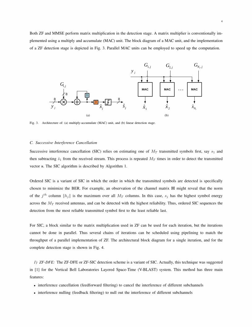
Both ZF and MMSE perform matrix multiplication in the detection stage. A matrix multiplier is conventionally im-

plemented using a multiply and accumulate (MAC) unit. The block diagram of a MAC unit, and the implementation

of a ZF detection stage is depicted in Fig. 3. Parallel MAC units can be employed to speed up the computation.

8

D

jiG,

jy js

8

8

D

jx

(a)

jyjG ,1 jG ,2 jNt

G ,

1x 2xtNx

MAC MAC MAC

(b)

Fig. 3. Architecture of: (a) multiply-accumulate (MAC) unit, and (b) linear detection stage.

C. Successive Interference Cancellation

Successive interference cancellation (SIC) relies on estimating one of MT transmitted symbols first, say s1 and

then subtracting s1 from the received stream. This process is repeated MT times in order to detect the transmitted

vector s. The SIC algorithm is described by Algorithm 1.

Ordered SIC is a variant of SIC in which the order in which the transmitted symbols are detected is specifically

chosen to minimize the BER. For example, an observation of the channel matrix H might reveal that the norm

of the jth column ‖hj‖ is the maximum over all MT columns. In this case, sj has the highest symbol energy

across the MT received antennas, and can be detected with the highest reliability. Thus, ordered SIC sequences the

detection from the most reliable transmitted symbol first to the least reliable last.

For SIC, a block similar to the matrix multiplication used in ZF can be used for each iteration, but the iterations

cannot be done in parallel. Thus several chains of iterations can be scheduled using pipelining to match the

throughput of a parallel implementation of ZF. The architectural block diagram for a single iteration, and for the

complete detection stage is shown in Fig. 4.

1) ZF-DFE: The ZF-DFE or ZF-SIC detection scheme is a variant of SIC. Actually, this technique was suggested

in [1] for the Vertical Bell Laboratories Layered Space-Time (V-BLAST) system. This method has three main

features:

• interference cancellation (feedforward filtering) to cancel the interference of different subchannels

• interference nulling (feedback filtering) to null out the interference of different subchannels

5

Input: received vector y, channel matrix H

Output: transmitted symbol s

begin

i←− 1

y(i) ←− y

H(i) ←− H = [hi,hi+1, . . . ,hMT]

for i← 1 to MT do

G(i) ←− (H(i)∗H(i) + σ2vI(MT−i+1)×(MT−i+1))

−1H(i)∗

xi ←− g(i)i y(i)

si ←− Q[xi]

y(i+1) ←− y(i) − sihiend

end

Algorithm 1: Algorithm for successive interference cancelation (SIC). g(i)i is an 1×MR vector representing the ith row of the (MT −

i+ 1)×MR matrix G(i).

MAC

)( i

jy

jiG,

8D

ijH ,

-

SIC iteration

)1( i

jy

D D

(a)

SIC Iter SIC Iter SIC Iter

1s 2s tNs

)2(

jy)3(

jy )( tN

jy)1(

jy

jG,1 1,jH jG ,2 2,jH jNtG , tNjH ,

D D D

(b)

Fig. 4. Architecture diagram of: (a) a single iteration stage, and (b) complete detection stage for a successive iteration cancelation receiver.

• subchannel ordering to reduce the effect of error propagation

Assuming that the received signal is of the form y = Hs + v, and that the matrix H is known at the receiver, we

can always decompose H into the product of a unitary matrix (Q) and an upper triangular matrix (R) via the QR

factorization. Thus, for the interference cancellation stage we left multiply the received vector y by Q∗ to obtain

y = Q∗y = Q∗(QRs + v) = Rs + v. After this step it easy to see that the decoder can begin detecting symbols

sequentially after detecting the symbol sMTfrom ˜yMT

= rMT ,MTsMT

+ vMTand nulling out its effect form the

others (interference nulling).

6

SIC, although simple and effective, suffers from what is known as error propagation since an error in decoding

any symbol will impact the detection of subsequent symbols. In fact, it can be shown that the performance of this

system is limited by the detection of the nth symbol (the nth subchannel) since the statistics of rn,n are the worst

(rn,n is χ square distributed with the least degrees of freedom). This is why improving the decoding of the nth

subchannel is crucial to improving the system performance.

D. Maximum Likelihood

The optimal MIMO detector is the maximum-likelihood (ML) detector. ML detector finds the most probable symbol

s that could have been transmitted given the received vector y. Under the assumption of additive white Gaussian

noise, and equally probable prior distribution for the symbol s, the ML detector chooses the nearest neighbor. Thus

the ML detector finds the solution to arg mins∈FMT ‖y−Hs‖. A straightforward implementation will perform an

exhaustive search over all FMT possible transmit vectors, which is prohibitively costly for high dimension systems.

ML achieves the optimal BER performance at the cost of exponential complexity.

E. Sphere Decoding

ML detection is an NP-hard problem, which means that all known solutions have a worst-case complexity that is

exponential in MT . However, the average complexity of a MIMO detector depends on the SNR, MT , and MR.

Because the received vector y is not arbitrary, but a point obtained by perturbing Gx with Gaussian noise n, the

average complexity is much less than the worst-case exponential complexity.

Many sophisticated algorithms have been developed to solve the ML problem. Historically the most widely used

algorithm is the Viterbi algorithm. However this algorithm is limited to Toeplitz matrices and is often used for

ISI SISO channels. There are other algorithms such as Kannan’s algorithm (which performs a search within a

parallelogram) [2], KZ algorithm [3] (which utilizes the Korkin-Zolotarev reduced basis), and the Fincke and Pohst

sphere decoding (SD) algorithm [4]. SD is the most efficient and attains polynomial time complexity in a large

number of cases (though the worst case is still exponential).

The basic idea for SD is to perform search over lattice points that lie within a sphere centered at the received

vector y. It is obvious that the closest lattice point within the sphere to the received vector r is also the closest

point among all the lattice points. This gives rise to two questions:

1) What should the radius r be? Determining the proper radius is important because, if the radius is too large,

the number of points needed to search for will be large, while if the radius is too small, no lattice points may

exist within the sphere.

7

2) Which points of the space lie within the sphere? This can be answered by testing the distance of each lattice

point to the received vector. Without a simple method to determine which points lie in the sphere, SD will be

no different from the original ML algorithm as every lattice point will need to be tested to determine if they

lie within the sphere or not.

SD does not give the answer to the first question, but it provides an efficient algorithm to determine the answer to

the second question. The basis of the algorithm is to transform the lattice points into a tree. A 16-QAM modulation

(with constellation points ±3±3j,±3±j,±1±j,±1±3j) with a 2-dimensional (MT = 2) sphere can be represented

as shown in Fig. 5. As seen in the figure, each branch corresponds to a constellation point, while the depth of the

tree equals the dimension. The number of leaves equal |FMT |, which is 162 for this example. By traversing the

tree from the root to the leaf, we obtain the complete symbol vector of a specific lattice point.

-3-j +3+j -3-3j -3-j +3+j -3-3j -3-j +3+j -3-3j -3-j +3+j

-3-3j -1-j +3+j+1+j

root

Fig. 5. Tree representation of a 16-QAM, 2-dimensional lattice.

Now if the distance from the received vector to a specific lattice point (the leaf of a tree) can be obtained by adding

the distance of each branch, we have an efficient tree based algorithm of determining which points lie within the

sphere. If the distance from the root to a particular node in the tree exceeds the sphere radius, we can conclude

that all leafs that have this particular node as a parent will lie outside the sphere. Thus we can successfully prune

all the branches below this node.

The tree representation of the lattice points does indeed have this branch metric property and the distance from the

root to a particular node is called the partial Euclidean distance (PED). While traversing down the tree, PED is a

non-decreasing value and the PED at the leaf equals the distance between the received vector and the lattice point.

To obtain the PED, the ML rule needs to be transformed. This process only needs to be done once for a specific

channel H and thus is often done in the preprocessing stage.

1) Preprocessor: Tree based detection algorithms first transforms the ML decoding rule through the QR decom-

position of the channel H = QR, where Q is unitary and R is upper triangle. The QR decomposition is done as

8

part of the preprocessing stage. As the norm is invariant to unitary transforms, the ML rule can be transformed as

follows

s = arg mins∈FMT

‖y −Hs‖ = arg mins∈FMT

‖QHy −Rs‖ = arg mins∈FMT

‖y −Rs‖ (7)

where y = QHy. Due to the triangular structure of R, the norm can now be rewritten as a sum of several vector

norms

‖y −Rs‖ =

MT∑

i=1

∣∣∣∣∣yi −MT∑

l=i

ri,lsl

∣∣∣∣∣

2

(8)

As the last MT − i+ 1 elements of summation only depend on the last MT − i+ 1 transmitted symbols and the

summation is non-decreasing, if this partial sum (partial Euclidean distance) exceeds the specified radius of the

sphere, it is safe to drop all candidate vectors that end with the same sequence of symbols. This is referred to tree

pruning.

2) Sphere Detector: Recently, tree-based sphere detectors (SD) have gained much interest as it enables the

search space to be restricted to the points that lie within a certain hyper-sphere centered around y. SD reduces the

complexity of ML significantly, but still the expected number of elements in the search space is still exponential in

the dimension of the MIMO system, thus application of SD at high dimensional systems are of great concern. Sphere

decoding (SD) algorithm has a close relation with tree based search algorithms where each node is associated with

a constellation point and traversing the tree from root to leaf gives the complete transmit vector. When a sphere

condition is violated, it can be thought of as pruning all branches below the current node. Through this process,

SD is capable of significantly reducing the search set.

3) Radius: The sphere radius is an important parameter that has considerable effect on the runtime complexity

of SD. For the SD to produce a meaningful result, the radius must be large enough to contain at least one leaf node.

However, if the radius is too large, SD converges to an exhaustive search ML. One reasonable value for the radius

is to use the distance between y and the ZF or MMSE solution. However, for ill conditioned channels, many points

may lie near the ZF solution and still cause the SD to iterate over a significant number of nodes. To even further

speed up the SD process, a dynamic radius maybe used where the radius is constantly updated to the minimum

value. This enables a larger number of nodes to be pruned resulting in lower complexity/higher throughput. In

dynamic radius reduction, the initial radius is often set to the distance of the first leaf node that is visited.

4) Node Ordering: In a constant radius SD algorithm, the order in which the nodes are visited has no impact on

complexity. However, for dynamic radius reduction, if nodes with smaller distances are visited first, the complexity

can be reduced significantly. Thus, proper ordering of the nodes is important. There have been many algorithms

proposed on the ordering of the nodes. The following are among the most significant ones.

1) Sorted QR

Sorted QR (SQRD) is done in the preprocessing stage. It is a modified version of the QR decomposition,

9

which sorts the columns so that the PED will be distributed in a manner where efficient pruning can be

obtained. SQRD is based on the Gram-Schmidt algorithm. Columns of H, Q, and R are reordered in each

orthogonalization step to minimize the diagonal element of R. This ensures that symbols with large hi (which

most likely have higher SNR) are detected first. The SQRD algorithm is given in Alg. 2.

Input: H

Output: Permutation matrix P and sorted QR decomposition Q and R of H

begin

R←− 0

Q←− H

P←− (1, ...,MT )

for i← 1 to MT do

ki = arg minl=i,...,MT‖qi‖2

exchange column i and ki in Q, R, and P

ri,i = ‖qi‖qi = qi/ri,i

for l← i+ 1 to MT do

ri,l = qHi ql

ql = ql − ri,lqlend

end

endAlgorithm 2: The sorted QR algorithm.

2) Schnorr/Euchner Ordering

When the tree is traversed depth first with dynamic radius reduction, if the depth-first strategy is supplemented

with the metric-first strategy, SD can be more efficient. This metric-first strategy is known as Schnorr/Euchner

(SE) ordering. The basic idea is to give preference to nodes with the smallest PED when choosing the next

parent node. By doing so, it is expected that leaf nodes with smaller PEDs will be found earlier which result

in rapid shrinkage of the sphere and more efficient pruning of the tree. There have been modified versions of

this algorithm that give different weight to the PED depending on the level of the tree. This is to compare the

PEDs equally, as PEDs that are closer to the leaf node are expected to be larger. For a real-valued constellation,

the SE ordering can be easily obtained by using geometric information. The constellation point that is closest

to the received vector will have the smallest PED. The ordering is then given in a zigzag fashion with the

received vector as the center point. This is illustrated in Fig. 6 for a 1-dimensional case.

10

r2Sphere constraint

Fig. 6. Schnorr/Euchner ordering for a 1 dimensional constellation.

3) PSK/QAM SE ordering

For a complex valued PSK or QAM constellation, SE ordering can be applied by performing a slight modifi-

cation. For PSK modulation, the distance from the received signal to a constellation point only depends on the

phase difference. This is because for PSK, all the constellation points are equidistant from the origin. Thus, SE

ordering can be performed by using the phase in place of the Euclidean distance. For QAM constellations, a

combination of PSK-SE ordering and exhaustive search is used. First, constellation points are grouped into sets

of equidistant points from the origin. For example, QPSK, 16-QAM, and 64-QAM yield 1, 3, and 9 PSK sets,

respectively. Then for each subset, the PSK SE ordering is obtained. Exhaustive search is performed among

the minimum distance point of each different PSK subsets to obtain the global minimum.

F. Sub-Optimal Detectors

1) K-best detection: The runtime complexity of SD is variable and depends highly on SNR. This is unfavorable

for VLSI implementations as it requires the hardware to be built assuming the worst case complexity, which is

equal to an exhaustive ML search. An alternative to SD is the K-Best detector. In K-Best, detection on the tree is

performed breadth first, and for each level, only the best K are retained. This gives a constant complexity algorithm,

but is now sub-optimal. However, its performance loss is small for sufficiently large K. Simulations show that for a

4×4 16-QAM system, K = 5 is a good tradeoff between performance and complexity, which is also verified by [5].

2) Combined ML and DFE Decoding: One technique to reduce the exponential complexity of the SD is to

combine linear detectors with optimal detectors to form a reduced complexity sub-optimal detector. In fact, combined

ML and DFE decoding, first introduced by [6], is one such technique. As the name implies, this detection scheme

combines the low computational complexity of SIC and the optimality of Maximum Likelihood. In its early form,

the authors proposed to decode the first p subchannels via ML decoding and use the DFE procedure to decode the

remaining subchannels in V-BLAST systems. The key idea of this detection scheme is to not perform a full QR

decomposition of H. In other words, the system does not completely upper triangulize the channel matrix as it is

11

typically done by the ZF-DFE receiver. If we only triangulize (n− p) columns of H we obtain

H = Q

R Ha

0 Hb

where Hb is a p× p square matrix, Ha is an (n− p)× p matrix, and R is an (n− p)× (n− p) upper triangular

matrix. Thus, the received signal, after left multiplying by Q, can be written as

y =

R Ha

0 Hb

sa

sb

+ v

Next, the scheme proceeds to jointly detecting the sub-vector sb = [sn−p+1, sn−p+2, ..., sn]T via a Maximum

Likelihood procedure. As SD did not exist at the time this work was presented, the authors used a full blown

ML to jointly detect these symbols. However, SD can be used for this step. After this step, the sub-vector

sa = [s1, ..., sn−p]T is detected by first canceling out the interference of sb and then using the usual DFE procedure.

It is clear that the choice of p has a direct impact on both the complexity and performance of this scheme and this

parameter is a key one that could be optimized when designing a combined ML and DFE detector.

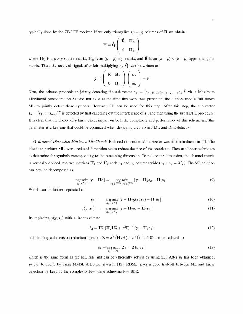
3) Reduced Dimension Maximum Likelihood: Reduced dimension ML detector was first introduced in [7]. The

idea is to perform ML over a reduced dimension set to reduce the size of the search set. Then use linear techniques

to determine the symbols corresponding to the remaining dimension. To reduce the dimension, the channel matrix

is vertically divided into two matrices H1 and H2 each n1 and n2 columns wide (n1+n2 = MT ). The ML solution

can now be decomposed as

arg mins∈FMT

‖y −Hs‖ = arg mins1∈Fn1 ,s2∈Fn2

‖y −H2s2 −H1s1‖ (9)

Which can be further separated as

s1 = arg mins1∈Fn1

‖y −H2g(y, s1)−H1s1‖ (10)

g(y, s1) = arg mins2∈Fn2

‖y −H2s2 −H1s1‖ (11)

By replacing g(y, s1) with a linear estimate

s2 = H∗2(H2H

∗2 + σ2I

)−1(y −H1s1) (12)

and defining a dimension reduction operator Z = σ2(H2H

∗2 + σ2I

)−1, (10) can be reduced to

s1 = arg mins1∈Fn1

‖Zy − ZH1s1‖ (13)

which is the same form as the ML rule and can be efficiently solved by using SD. After s1 has been obtained,

s2 can be found by using MMSE detection given in (12). RDML gives a good tradeoff between ML and linear

detection by keeping the complexity low while achieving low BER.

12

III. SOFT-INPUT SOFT-OUTPUT MIMO DETECTORS

A. Introduction

Different classes of hard MIMO detectors were described in section II. Specifically, linear and optimal detectors were

discussed and it was shown that although linear detectors benefit from the reduced computational complexity, they

perform poorly especially at moderate to low values of SNR. In addition, it was also shown that there exists a class

of sub-optimal hard detectors which attempts to combine the good features of both linear and optimal detectors. In

this section, we will study another category of MIMO detectors commonly known as soft-input soft-output (SISO)

MIMO detectors. This category of detectors is exclusively used in MIMO communication systems following the

turbo principle [8]. In fact, turbo systems were first introduced by Berrou et al. as a promising technique to approach

the Shannon capacity for an additive white Gaussian noise (AWGN) channel. This concept was then extended to

include MIMO systems. Hence, a new field of iterative detection and decoding (IDD) for multiple antenna channels

was born [9]. In an IDD receiver, soft information is exchanged between the symbol detector and the channel decoder

to achieve performance close to channel capacity. In this section, we will focus on describing several classes of

soft symbol detectors for multi antenna channels and keep the discussion on MIMO channel decoders for section IV.

B. Soft Detectors

At the transmitter, a rate R code is used to convert a vector of i.i.d. bits b to an encoded vector of bits c. While

the entries of b are independent, the entries of c are clearly dependent. This is why the vector of encoded bits is

then multiplexed to different layers (MT layers) via a serial to parallel converter and interleaved via a random (or

deterministic) interleaving matrix. Hence, we obtain MT vectors of encoded bits {ci}MTi=1 that are almost independent

due to interleaving. In the sequel, we will assume that the encoded and reshuffled bits are independent. The last

stage at the transmitter is the modulation stage. The modulation format used on the LTE-A uplink is single carrier

frequency domain multiple access (SC-FDMA). At the receiver, the first two stages are down conversion and

demodulation. Since LTE-A systems use SC-FDMA for modulation, the demodulation procedure should be be

tailored to this modulation technique. After down-conversion and demodulation, we know, from section II, that the

received signal vector is given by y = Hs+v. Assuming that each symbol sk belongs to a 2q-ary QAM alphabet,

we label the bits associated with sk by ck,1, ck,2, ..., ck,q . Thus, the symbol vector s comprises of qMT bits. The

task of the soft symbol detector is to compute the a posteriori log-likelihood ratio (APLLR) for each bit. Note

that the received symbol vector constitutes of qMT bits. Assuming a spatially additive white Gaussian noise, the

APLLR is defined as and given by

Lpost(ck,i) = logP (ck,i = +1|y)

P (ck,i = +1|y)= log

∑s∈S+

k,ie−d(s)/σ

∑s∈S−

k,ie−d(s)/σ

(14)

where

d(s) = ||y −Hs||2 − σMT∑

i=1

q∑

j=1

logP (ci,j)

13

P (ci,j) =1

2(1 + ci,j tanh(

Lpri(ci,j)

2))

The set S+k,i is the set of all symbols satisfying ck,j = +1 (S−k,i is defined similarly), and Lpri(ck,i) is the a priori

log-likelihood ratio defined as

Lpri(ck,i) = logP (ck,i = +1)

P (ck,i = −1)(15)

The symbol detector receives a symbol vector y, computes the APLLRs assuming equal priors on all transmitted

bits ck,i, and passes the soft information to the channel decoder which in turn computes the new priors and feeds

them back to the symbol detector. This process is iterated until a certain convergence criterion is met. At that point,

the ALLRs are quantized and consequently, hard decisions are made.

C. Soft Sphere and Tree based Detectors

After outlining the basic role of a soft MIMO detector, we now focus on discussing different implementations of

such detector. Ultimately, we are seeking a device that, given a received vector y and a priori likelihood ratios,

outputs an updated version of the a posteriori likelihood ratios (ALLRs). One way to solve for the ALLRs is to

derive a soft-input soft-output detector that solves for the exact ALRRSs via a brute force search over all s ∈ FMT .

The task of this detector is to compute

Lpost(ck,i) = log

∑s∈S+

k,ie−d(s)/σ

∑s∈S−

k,ie−d(s)/σ

for each bit. This computation, however, requires searching over all s ∈ FMT to obtain the sets S+k,i and S−k,i and

then marginalizing the a posteriori probabilities over these sets. This, of course, is computationally prohibitive and

not implementable for large block codes and/or large signal constellations. In this section, we show how the hard

sphere decoder, which finds the hard ML estimate using tree based search algorithms, can be altered to output the

ALLRs of the bits comprising the received vector. First we recall, from section II-E, that a sphere decoder computes

the following path metric

p(s) = ‖y −Rs‖ =

MT∑

i=1

∣∣∣∣∣yi −MT∑

l=i

ri,lsl

∣∣∣∣∣

2

(16)

for a collection of symbols living inside a sphere of radius B via a breadth first search or depth first search

algorithm. Afterwards, the decoder chooses the symbol vector with the smallest path metric as the quantized (hard)

decision. While this procedure requires less computations relative to the full hard ML detector it still suffers from

an expected exponential computational complexity. In order to derive the soft sphere detector we start by obtaining

a relationship between d(s) and p(s). If we recompute d(s) while taking the QR factorization of the channel matrix

H into account

d(s) = ||y −Rs||2 − σMT∑

i=1

q∑

j=1

logP (ci,j) =

MT∑

i=1

(p(si)− σ

q∑

j=1

logP (ci,i)

)+ C

14

where p(si) =∣∣∣yi −

∑MT

l=i ri,lsl

∣∣∣2

and si = [si, si+1, ..., sMT]T is the partial symbol vectors (PSVs) as in [10].

Note that since the constant term C appears in d(s) for all s we can drop it with out loss of optimality. In addition,

since we are summing over the PSVs, they can be arranged in a tree that has its root just above level i = MT

and leaves, on level i = 1, which correspond to symbol vectors s. The Euclidean distances d(s) can be computed

recursively as d(s) = d1 with the partial Euclidean distances (PEDs) di = di+1 + |ei|2 , i = MT ,MT − 1, ..., 1,

where dMT+1 = 0 and the distance increments (DIs)

|ei|2 = |y −MT∑

j=i

ri,jsj |2 (17)

Since the dependence of the PEDs di on the symbol vector s is only through the PSV si, we have transformed the

soft ML detection and the computation of the ALLRs into a weighted tree-search problem: PSVs and PEDs are

associated with nodes, branches correspond to DIs. Using d(s), the tree detection algorithm compares the reliability

of distinctive paths and chooses the surviving paths. In other words, the tree detection algorithm finds the complete

paths associated with smallest d(s). Denoting the set of the corresponding symbol candidates as L, the approximate

ALLRs can be expressed as

Lpost(ck,i) ≈ log

∑s∈L∩S+

k,ie−d(s)/σ

∑s∈L∩S−

k,ie−d(s)/σ

(18)

We can also use the max-log approximation to further simplify the above approximation

Lpost(ck,i) ≈(

mins∈L∩S+

k,i

d(s)− mins∈L∩S−

k,i

d(s)

)(19)

Although soft sphere detectors and tree based detectors are less complex relative to a soft ML detector they still have

an exponential computational complexity which is not desirable for large number of antennas and/or large signal

signal constellations. This is why, we will next study some simpler sub-optimal techniques that achieve reduced

complexity. Finally, it is important to mention that in the case when there is no passing of soft information back

and forth between the channel detector and the channel decoder, the soft sphere decoder assumes equal priors on

bits and the max-log approximation becomes

Lpost(ck,i) ≈(

mins∈L∩S+

k,i

||y −Rs||2 − mins∈L∩S−

k,i

||y −Rs||2)

(20)

D. Soft MMSE Detector

In order to reduce the computational burden imposed by a soft ML or sphere decoder, a soft MMSE detector could

be used [11]. As we already know, the task of the soft channel detector is to calculate the ALLRs given the a priori

distribution of the transmitted bits and the received signal vector. Instead of solving for the exact ALLRs, one could

use a linear MMSE detector to first estimate the transmitted symbols and then compute the ALLRs based on this

estimate. We start deriving the soft MMSE by rewriting the received signal as

y = hksk + Hksk + n (21)

15

where Hk = [h1h2, ...,hk−1,hk+1, ...,hMr], and sk = [s1, s2, ..., sk−1, sk+1, ..., sMr

]. The decision statistic of the

kth substream using a linear filter wk is

yk = w∗ky = dk + uk + vk (22)

where dk = w∗khksk is the desired response obtained by linear beamforming, uk = w∗kHksk is the co-antenna

interference (CAI), and vk = w∗kv is the phase rotated noise respectively. In this scheme, the CAI is removed

from the linear beamformer output to obtain xk = yk − uk where uk is the linear combination of interfering

substreams and xk is the improved estimate of transmitted symbol sk. As proposed in [11], the multisubstream

detector optimizes the interference estimate and the weights of the linear detector jointly. The performance of the

estimator is measure by the error ek = sk − xk. The weights wk and the interference estimate uk are optimized

by minimizing the mean-square value of the error between each substream and its estimate

(wk, uk) = arg minwk,uk

E[||sk − xk||2] (23)

where the expectation E is taken over the noise and the statistics of the data sequence. The solution to the problem

is given by

wk = (P + Q + ΣMR)−1hk (24)

uk = w∗kz (25)

where

P = hkh∗k

Q = Hk[I(MR−1) − diag(E[sk]E[sk]∗)]H∗k

ΣMR= σ2IMR

z = HkE[sk]

In solving for E[sk], the relationship between the expectation and the a priori distributions is given by

E[ck,j ] = tanh

(Lpri(ck,j)

2

), j = 1, 2, ..., B

In arriving to the above solution, it was assumed that E[vv∗] = σ2IMR, E[sv] = 0, and E[sisj ] = E[si]E[sj ]

∀i 6= j. These conditions are achieved via independent and different space and time interleaving at the transmitter.

For the first iteration, it is assumed that E[sk] = 0, in which case xk is given by

xk = h∗k(HH∗ + σ2I)−1y

With increasing number of iterations, we assume that in the limit, E[sk]→ sk, in which case, xk simplifies to

xk = (h∗khk + σ2)−1σ∗k(y −Hksk)

due to the perfect soft interference canceler. Finally, to acquire the expectations of interfering substreams, we use

the a priori distributions of the transmitted bit streams provided by the channel decoder at the previous iteration.

16

IV. CHANNEL DECODERS

A. Convolutional Codes

1) Encoding: Convolutional codes are encoded by using a linear feedback shift register (LFSR). A convolutional

code is defined by the number of memory elements and the topology of the feedback and feedforward network,

which is represented in compact form by the generator polynomial. A simple convolutional encoder is shown in

Fig. 7.

Fu-hua Huang Chapter 2. Convolutional Codes 5

where k is the number of parallel input information bits and n is the number of paralleloutput encoded bits at one time interval. The constraint length K for a convolutional codeis defined as

K m= + 1 (2.2)where m is the maximum number of stages (memory size) in any shift register. The shiftregisters store the state information of the convolutional encoder and the constraint lengthrelates the number of bits upon which the output depends. For the convolutional encodershown in Figure 2.1, the code rate r=2/3, the maximum memory size m=3, and theconstraint length K=4.

A convolutional code can become very complicated with various code rates andconstraint lengths. As a result, a simple convolutional code will be used to describe thecode properties as shown in Figure 2.2.

DD

+

+

c(2)

c(1)

x(1)

Figure 2.2: Convolutional encoder with k=1, n=2, r=1/2, m=2, and K=3.

2.2 Encoder Representations

The encoder can be represented in several different but equivalent ways. They are1. Generator Representation2. Tree Diagram Representation3. State Diagram Representation4. Trellis Diagram Representation

Fig. 7. A simple convolutional encoder with memory size 2, and rate 1/2.

2) Decoding: Several algorithms exist for decoding convolutional codes. For relatively small values of k, the

Viterbi algorithm is universally used as it provides maximum likelihood performance and is highly parallelizable.

Viterbi decoders are thus easy to implement in VLSI hardware and in software on CPUs with SIMD instruction sets.

Longer constraint length codes are more practically decoded with any of several sequential decoding algorithms, of

which the Fano algorithm is the best known. Unlike Viterbi decoding, sequential decoding is not maximum likelihood

but its complexity increases only slightly with constraint length, allowing the use of strong, long-constraint-length

codes.

Both Viterbi and sequential decoding algorithms return hard-decisions: the bits that form the most likely codeword.

An approximate confidence measure can be added to each bit by use of the soft output Viterbi algorithm. Maximum

a posteriori (MAP) soft-decisions for each bit can be obtained by use of the BCJR algorithm.

B. Turbo Codes

Turbo codes were first introduced in 1993 by Berrou, Glavieux, and Thitimajshima [12], and were among the first

codes to achieve near capacity.

17

Information sequence

Interleaver

Systematic Output

Conv.

Encoder

Conv.

Encoder

Output I

Output II

Parity Output

Fig. 8. A turbo encoder (parallel concatenated convolutional code).

Interleaver

Decoder

Parity Data 2

Systematic Data

Interleaver

Soft Information

Decoder

DeinterleaverSoft

Information

Parity Data 1

Fig. 9. A turbo decoder. Exchange of soft information is the key to its high performance.

1) Encoding: Turbo codes are constructed as a combination of two or more component codes on different

interleaved version of the same information sequence. Turbo encoding is usually done by encoding the information

sequence using a convolutional code, then interleaving the sequence, and finally performing another convolutional

encoding on the interleaved sequence. The first convolutional code consists the outer code, while the second code

is the inner code. This process is depicted in Fig. 8

2) Decoding: Turbo decoding is performed by using an iterative decoder. A high level block diagram is given in

Fig. 9. For each constituent code, a separate decoder exists. Each decoder outputs soft information of the decoded

bits. The other decoder uses this soft information as its a posteriori probability. Decoding continues for a number

of iterations until the outputs converge, or a certain criterion is met.

V. ITERATIVE MIMO RECEIVER

In an iterative turbo MIMO receiver, the main concept is the same as that of the turbo decoder shown in Fig. 9. Turbo

principles can be applied to any system with a channel code as the outer code, while the inner code is considered

to be the channel effects. This is true for turbo equalizers where the inner code of the serial concatenated turbo

code is assumed to be the inter-symbol-interference (ISI) channel. Here the inner code is defined as a rate 1 code

over the field of real or complex numbers. The concept of such an iterative turbo equalizer has been demonstrated

18

and shows perfect equalization for a multipath Gaussian channel [13].

Extending the turbo principle to MIMO detection, the spatial multiplexing of a MIMO channel can be viewed as

the inner code, while there exists an outer code, a turbo code in the case of LTE-A systems. Thus, the crux of a

turbo MIMO receiver lies in the development of a soft-input soft-output MIMO detector, along with an efficient

iterative structure that can pass information between the channel decoder and the MIMO detector. The fundamental

structure of such a receiver is shown in Fig. 10.

Channel

Encoder

InterleaverΠ

Mapper

SISO MIMO

Detector

TM

RM

DeinterleaverΠ-1

Channel Decoder

InterleaverΠ

Data Source

Data Sink

Fig. 10. Fundamental architecture of an iterative turbo MIMO receiver.

A. Turbo BLAST

One of the first work on turbo MIMO receiver is the work done by Sellathurai and Haykin [11]. In this work,

Bell labs layered space time (BLAST) is extended and casted in the context of turbo decoding. Foschini has

answered the fundamental question of constructing a BLAST system whose capacity grows linearly with the

number of transmit antennas. D-BLAST was the solution to this problem. However, D-BLAST is too complex

for any practical implementation. Turbo-BLAST plays an important role in reducing the complexity of D-BLAST

for practical implementations.

In turbo-BLAST, a random space-time block (RSTB) code is used. RSTB is implemented by first encoding

substreams using independent FEC codes. A following space-time random interleaver is used to create an inter-

stream permutation. The space-time interleaver first interleaves in time, then permutes across space. The space

interleaver ensures the spatial cycling of each substream over all possible sub channels (transmit antennas).

19

In theory, the RSTB code can be modeled as a single Markov process, and a trellis can be formed that includes

the effect of interleaving. However, such a trellis representation is extremely complex and no feasible decoding is

possible. Borrowing from turbo principles, the FEC code is considered as an outer code, while the wireless channel

(a time varying matrix channel) is viewed as an inner code. This is depicted in Fig. 11.

Fig. 11. RSTB codes as a serially concatenated code. Courtesy of Sellathurai et al. [11].

In an iterative decoding scheme, the two decoding stages will be a SISO detector for the inner code, and a

set of parallel SISO channel decoders for the outer code. The two stages are separated by the space-time inter-

leaver/deinterleaver. This process is depicted in Fig. 12.

As the soft detector, several choice can be used. The optimal detector is the MAP detector, where the probability of

the kth substream is obtained by averaging out the contributions of the interfering substreams. As is with any MAP

scheme, the complexity of the soft MAP detector is large, and exponential with the number of transmit antennas.

However, a sub-optimal scheme that employs the max-log approximation can be used.

Any standard SISO decoder for the employed FEC code can be used as the outer decoder. The performance of the

turbo-BLAST system is shown in Fig. 13.

B. MMSE Turbo Receiver

A different frequency-selective fading channel has been considered in [14]. In this paper, coding is introduced in

space and frequency dimension by means of bit-interleaved coded modulation (BICM). To perform the MIMO space

20

Fig. 12. Iterative decoder for turbo-BLAST. Courtesy of Sellathurai et al. [11].

Fig. 13. Performance of Turbo-BLAST. Courtesy of Sellathurai et al. [11].

equalization, a set of SISO MMSE equalizers are used which perform demodulation as well. The soft information

is exchanged between the SISO MMSE equalizer and the channel decoder in a turbo principle. Overall, OFDM

is used to convert the frequency selective channel to several flat fading channels. The basic block diagram of the

transmitter is given in Fig. 14.

The iterative receiver employs the turbo principles by using a SISO outer decoder and a soft output space equal-

21

int.conv. mapper

mapper

demux.encoder

mapper

xb xc

x(1)d

x(nT )d

s(1)p

s(2)p

s(nT )p

ua

ofdm g(t)

g(t)

g(t)

ofdm

ofdm

x(2)d

Fig. 1. Transmitter structure

permutation. The frame of interleaved coded bits is then splitinto nT sub-blocks. Within each of these sub-blocks, Q bitsx(i)d are grouped and mapped, with the mapping function µ,

to one of the M = 2Q possible complex symbols in theconsidered multilevel/phase constellation S (e.g. M-PSK, M-QAM,. . . ) :

s(i)p = µ(x(i)p·Q+1, . . . , x

(i)p·Q+Q). (1)

The resulting length-nC frame of complex symbols s(i)p ∈ S

(i = 1, . . . , nT , p = 0, . . . , nC − 1) enters a classical OFDMmodulator (IFFT followed by CP insertion) of nC carriers.The symbols s

(i)p have zero mean and variance σ2

s . Thesamples obtained after OFDM modulation are serial to parallelconverted, enter a square-root Nyquist pulse shaping filter g(t)and are transmitted at a rate 1/T .

Frequency diversity is exploited here thanks to the codingintroduced prior to interleaving and stream splitting. Moreover,the presence of a bit-interleaver greatly reduces the correlationbetween successive coded bits and, in combination with theencoder, enables to use the turbo principle at the receiver. Wecan thus talk of a bit-interleaved space-frequency code whichadmits iterative turbo processing at the receiver. Note also thatthis scheme offers high flexibility because the encoder and themodulation can be chosen independently.

Since we assume that the transmitter does not have anyknowledge of the channel impulse responses, the same bitloading and power loading is used for any carrier of any trans-mit antenna. The mapping rule is also the same everywhere.

III. CHANNEL MODEL

We consider frequency-selective MIMO fading channelsmodeled as tapped-delay lines. The different paths are char-acterized by gains (independent zero-mean complex gaussianrandom variables with tap-specific variances) and delays. Weassume quasi-static Rayleigh fading, which means that thechannel taps remain constant over a frame of transmittedsymbols (which is a reasonable assumption for relatively smallframes). From one frame to another, the channel taps areassumed to vary independently.

The lowpass equivalent channel impulse response (includingthe shaping filter g(t) and the physical multipath channel)between transmit antenna i (i = 1, . . . , nT ) and receiveantenna j (j = 1, . . . , nR) is denoted by h(j,i)(t). We assumeh(j,i)(t) is of finite duration. At receive antenna j, r(j)(t)denotes the received signal and n(j)(t) is the complex envelopeof an additive white gaussian noise with two-sided powerspectral density (psd) N0/2.

int.

decoder

deint.P/S

S/P

r(nR)l

tone nC − 1

r(1)l

tone 0ofdm−1

ofdm−1

Space-equalizer

Space-equalizer

La

(x(i)0·Q+b

)

ua

y(1)1

Le

(x(i)(nC−1)·Q+b

)

Le(xc)

La(xc) Le(xb)

Lp(ua)

La(xb)

y(nR)nC

Fig. 2. Receiver structure

Assuming that the CP is longer than the longest channelimpulse response and proper FFT alignment, interferencebetween successive OFDM symbols is avoided. Besides, de-noting by yjp(n) the sample at the pth FFT output at receiveantenna j when the nth OFDM symbol is processed, we have

yjp(n) =

nT∑

i=1

H(j,i)p (n) sip(n) + nj

p(n) (2)

where sip(n) denotes the symbol transmitted on carrier p of

the ith antenna in the nth OFDM symbol, and H(j,i)p (n) is the

complex channel gain for tone p between transmit antenna iand receive antenna j during the transmission of the OFDMsymbol n. The additive noise is denoted by nj

p(n). A vectormodel can be obtained by stacking together input and outputvalues. Omitting the symbol index n, we denote by sp (forp = 1, . . . , nC ), the vector of transmitted symbols on tone p,by y

p(resp. np) the vector of received samples on tone p

(resp. noise samples) obtained after FFT. It comes

sp � [s(1)p . . . s(nT )p ]T(nT×1), (3)

yp� [y(1)p . . . y(nR)

p ]T(nR×1), (4)

np = [n(1)p . . . n(nR)

p ]T(nR×1). (5)

The observation model then becomes:

yp= H

psp + np, (6)

where [H

p

]ji= H(j,i)

p (n). (7)

IV. ITERATIVE RECEIVER

The receiver is iterative and makes use of the turbo prin-ciple. For the sake of simplicity, we assume perfect channelknowledge and perfect synchronization. As represented in Fig.2, the receiver is made of the association of two SISO stages,separated by bit (de)interleavers, exchanging extrinsic infor-mation under the form of bit log-likelihood ratio’s (LLR’s).

The SISO binary decoder is the classical outer SISO stagefound in turbo receivers built in analogy with the decoding ofa serial concatenated turbo code. It is classically implementedusing an a posteriori probability (APP) algorithm in thelogarithmic domain, based on the BCJR algorithm [10].

The inner SISO stage is actually a set of nC stages,operating carrier-wise, and having to mitigate co-antenna inter-ference (CAI) and to properly demodulate the symbols. These

Fig. 14. Transmitter for MMSE turbo. Courtesy of Zuyderhoff et al. [14].

izer/demodulator which is separated by an interleaver and deinterleaver as depicted in Fig. 15. The outer decoder

simply implements the SISO convolutional decoder based on the BCJR algorithm. The inner SISO equalizer needs

to mitigate the spatial interference as well as properly demodulate the symbols. By assuming the independence of

the interleaved and demultiplexed coded bits, the two stages can be split as shown in Fig. 16.

int.conv. mapper

mapper

demux.encoder

mapper

xb xc

x(1)d

x(nT )d

s(1)p

s(2)p

s(nT )p

ua

ofdm g(t)

g(t)

g(t)

ofdm

ofdm

x(2)d

Fig. 1. Transmitter structure

permutation. The frame of interleaved coded bits is then splitinto nT sub-blocks. Within each of these sub-blocks, Q bitsx(i)d are grouped and mapped, with the mapping function µ,

to one of the M = 2Q possible complex symbols in theconsidered multilevel/phase constellation S (e.g. M-PSK, M-QAM,. . . ) :

s(i)p = µ(x(i)p·Q+1, . . . , x

(i)p·Q+Q). (1)

The resulting length-nC frame of complex symbols s(i)p ∈ S

(i = 1, . . . , nT , p = 0, . . . , nC − 1) enters a classical OFDMmodulator (IFFT followed by CP insertion) of nC carriers.The symbols s

(i)p have zero mean and variance σ2

s . Thesamples obtained after OFDM modulation are serial to parallelconverted, enter a square-root Nyquist pulse shaping filter g(t)and are transmitted at a rate 1/T .

Frequency diversity is exploited here thanks to the codingintroduced prior to interleaving and stream splitting. Moreover,the presence of a bit-interleaver greatly reduces the correlationbetween successive coded bits and, in combination with theencoder, enables to use the turbo principle at the receiver. Wecan thus talk of a bit-interleaved space-frequency code whichadmits iterative turbo processing at the receiver. Note also thatthis scheme offers high flexibility because the encoder and themodulation can be chosen independently.

Since we assume that the transmitter does not have anyknowledge of the channel impulse responses, the same bitloading and power loading is used for any carrier of any trans-mit antenna. The mapping rule is also the same everywhere.

III. CHANNEL MODEL

We consider frequency-selective MIMO fading channelsmodeled as tapped-delay lines. The different paths are char-acterized by gains (independent zero-mean complex gaussianrandom variables with tap-specific variances) and delays. Weassume quasi-static Rayleigh fading, which means that thechannel taps remain constant over a frame of transmittedsymbols (which is a reasonable assumption for relatively smallframes). From one frame to another, the channel taps areassumed to vary independently.

The lowpass equivalent channel impulse response (includingthe shaping filter g(t) and the physical multipath channel)between transmit antenna i (i = 1, . . . , nT ) and receiveantenna j (j = 1, . . . , nR) is denoted by h(j,i)(t). We assumeh(j,i)(t) is of finite duration. At receive antenna j, r(j)(t)denotes the received signal and n(j)(t) is the complex envelopeof an additive white gaussian noise with two-sided powerspectral density (psd) N0/2.

int.

decoder

deint.P/S

S/P

r(nR)l

tone nC − 1

r(1)l

tone 0ofdm−1

ofdm−1

Space-equalizer

Space-equalizer

La

(x(i)0·Q+b

)

ua

y(1)1

Le

(x(i)(nC−1)·Q+b

)

Le(xc)

La(xc) Le(xb)

Lp(ua)

La(xb)

y(nR)nC

Fig. 2. Receiver structure

Assuming that the CP is longer than the longest channelimpulse response and proper FFT alignment, interferencebetween successive OFDM symbols is avoided. Besides, de-noting by yjp(n) the sample at the pth FFT output at receiveantenna j when the nth OFDM symbol is processed, we have

yjp(n) =

nT∑

i=1

H(j,i)p (n) sip(n) + nj

p(n) (2)

where sip(n) denotes the symbol transmitted on carrier p of

the ith antenna in the nth OFDM symbol, and H(j,i)p (n) is the

complex channel gain for tone p between transmit antenna iand receive antenna j during the transmission of the OFDMsymbol n. The additive noise is denoted by nj

p(n). A vectormodel can be obtained by stacking together input and outputvalues. Omitting the symbol index n, we denote by sp (forp = 1, . . . , nC ), the vector of transmitted symbols on tone p,by y

p(resp. np) the vector of received samples on tone p

(resp. noise samples) obtained after FFT. It comes

sp � [s(1)p . . . s(nT )p ]T(nT×1), (3)

yp� [y(1)p . . . y(nR)

p ]T(nR×1), (4)

np = [n(1)p . . . n(nR)

p ]T(nR×1). (5)

The observation model then becomes:

yp= H

psp + np, (6)

where [H

p

]ji= H(j,i)

p (n). (7)

IV. ITERATIVE RECEIVER

The receiver is iterative and makes use of the turbo prin-ciple. For the sake of simplicity, we assume perfect channelknowledge and perfect synchronization. As represented in Fig.2, the receiver is made of the association of two SISO stages,separated by bit (de)interleavers, exchanging extrinsic infor-mation under the form of bit log-likelihood ratio’s (LLR’s).

The SISO binary decoder is the classical outer SISO stagefound in turbo receivers built in analogy with the decoding ofa serial concatenated turbo code. It is classically implementedusing an a posteriori probability (APP) algorithm in thelogarithmic domain, based on the BCJR algorithm [10].

The inner SISO stage is actually a set of nC stages,operating carrier-wise, and having to mitigate co-antenna inter-ference (CAI) and to properly demodulate the symbols. These

Fig. 15. Receiver for MMSE turbo.

computation of symbola priori probabilities

spacedemodulator

mux.

equalizer

Pe(s(i)p )

Pa(s(i)p )

Le

(x(i)p·Q+b

)

y(nR)p

y(1)p

La

(x(i)p·Q+b

)

Fig. 3. Space-equalizer Stage

first two tasks are achieved by the space equalizer. Assumingindependence of the interleaved and demultiplexed coded bitsat the transmitter, space equalization and demodulation maybe split as represented in Fig. 3. On the basis of the receivedsamples defined in section III and of the symbols a prioriprobabilities Pa(s

(i)p ) (i = 1, . . . , nT ; p = 0, . . . , nC − 1),

the SISO space equalizer associated with carrier p outputs thesymbol extrinsic probabilities Pe(s

(i)p ) � κsPp(s

(i)p )/Pa(s

(i)p ),

where Pp(s(i)p ) are the APP of symbol s

(i)p and κs is a

normalization constant.The required symbol a priori probabilities can be computed

from the available a priori bit LLR’s. On the basis of the sym-bol extrinsic probabilities obtained at the output of the SISOspace equalizer, the demapper (demodulator) can optimallycompute the extrinsic LLR’s of the coded bits. The details ofthese operations can be found in [11].

We apply here a low-complexity MMSE solution derivedfrom the work reported in [11] instead of the optimal trellis-based solution. In this context, a linear block operation isused in order to produce an estimate s

(i)p for each transmitted

symbol s(i)p . However, in order to keep the analogy with an

optimal BCJR-based implementation, the a priori informationPa(s

(i)p ) available about transmitted symbol s

(i)p cannot be

used in order to compute its estimate s(i)p , so that the extrinsic

probabilities Pe(s(i)p ) approximated on the basis of s

(i)p will

not depend on Pa(s(i)p ). Respecting this constraint, we search

the optimal solution according to the MMSE criterion (i.e.minimizing the mean square error E{|s(i)p − s

(i)p |2}). For the

sake of conciseness, we refer the reader to [11] for a completederivation of what follows. The equalizer structure derivedhere belongs to the same family to whom belongs the solutionproposed in [9].

The solution makes use of the symbol mean s(i)p and

variance v(i)p , which can be estimated on the basis of the

available a priori information (see [11]). We define the length-nT mean vector s(i)p and the square covariance matrix R(i)

ss,pof size nT × nT :

s(i)p � [s(1)p . . . s(nT )p ]T , (8)

R(i)

ss,p= diag[v(1)p . . . v(i−1)

p σ2s v

(i+1)p . . . v(nT )

p ]. (9)

After some calculation, the solution may be expressed as:

s(i)p = w(i)p

H[yp−H s(i)p

], (10)

with the time-varying complex filter w(i)p given by:

w(i)p = σ2

s [HR(i)

ss,pHH + σ2

nI]−1H e(i). (11)

I is the identity matrix of size nR×nR and e(i) is a selectingvector nR × 1 with line i at 1 and others filled in with 0s.

As in [9], we assume that the estimate s(i)p is the output of

an equivalent AWGN channel having s(i)p at its input:

s(i)p = µ(i)p s(i)p + η(i)p with η(i)p ∼ Nc(0, ν

(i)p

2). (12)

The parameters µ(i)p and ν

(i)p

2can be calculated for each

transmitted symbol s(i)p as a function of the filter w(i)p [11]:

µ(i)p = w(i)

p

HH e(i) and ν(i)p

2= µ(i)

p σ2s − µ(i)

p

2σ2s . (13)

Using the gaussian equivalent channel assumption given in(12), we can then approximate the symbol extrinsic proba-bilities Pe(s

(i)p ) at the output of the SISO space equalizer as

[11]:

Pe(s(i)p ) ∼ p(s(i)p |s(i)p ) =

1

ν(i)p

2πexp

[−|s(i)p − µ

(i)p s

(i)p |2

ν(i)p

2

].

(14)The demapper can finally compute the bit extrinsic LLR’sneeded at the input of the SISO decoder (see [11]).

In order to compare this low-complexity solution with theoptimal one, we also derive a space-equalizer based on theMAP criterion (see [8] for a non-OFDM MAP receiver). Wehave to compute the a posteriori probabilities Pp(x

(i)p·Q+b) �

P (x(i)p·Q+b|yp

) of the bth coded bit of symbol s(i)p . Using Bayesrule, we find

Pp

(x(i)p·Q+b = ±1

)=

∑

sp∈S(i)p,b,±1

P(yp| sp)Pa

(sp)

(15)

where S(i)p,b,±1 denotes the set of possible symbol combinations

on the nT tones with index p, for which the bth bit of symbols(i)p , bit x(i)

p·Q+b, is either +1 or −1. Explicitly we have

Pp

(x(i)p·Q+b = ±1

)=

∑

sp∈S(i)p,b,±1

(exp

(− 1

N0

nR∑

r=1

∣∣∣yrp −nT∑

t=1

H(r,t)p s(t)p

∣∣∣2)

nT∏

t=1

log2 M∏

m=1

Pa(x(t)p·Q+m = ±1)

)(16)

and the corresponding log-likelihood ratio (LLR) becomes

LLR(x(i)p·Q+b

)= ln

(Pp(x

(i)p·Q+b = +1)

Pp(x(i)p·Q+b = −1)

). (17)

The MAP space-frequency equalizer/demapper has been im-plemented by means of the log-MAP algorithm and we sendextrinsiq LLR to the decoder.

Fig. 16. Space equalizer for MMSE turbo. Courtesy of Zuyderhoff et al. [14].

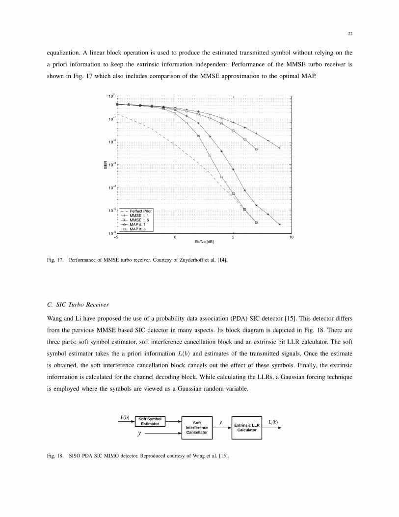
For the equalization, a low complexity MMMSE solution is derived based on the optimal trellis approach of turbo

22

equalization. A linear block operation is used to produce the estimated transmitted symbol without relying on the

a priori information to keep the extrinsic information independent. Performance of the MMSE turbo receiver is

shown in Fig. 17 which also includes comparison of the MMSE approximation to the optimal MAP.

−5 0 5 1010

−6

10−5

10−4

10−3

10−2

10−1

100

Eb/No [dB]

BE

R

Perfect PriorMMSE it. 1MMSE it. 6MAP it. 1MAP it. 6

Fig. 4. Influence of receiver: MAP and MMSE.

V. SIMULATION RESULTS

This section is devoted to the presentation of performanceresults in several configurations. All the simulations have thefollowing common parameters. The frame size is 574 infor-mation bits. The convolutional encoder, of constraint length3 and octal generator polynomials [58, 78], always begins andends a frame at the all-zero state (i.e. trellis termination isperformed). The interleaver is totally random and no trial ismade to optimize it. The modulation is 8-PSK with Grayor set partitioning (SP) mapping. OFDM has 64 carriers butonly 48 used (Hiperlan standard). The pulse shaping filter isa square-root raised cosine filter with a 0.3 roll-off factor.The nT transmit antennas send signals with equal power. Ifthe excess bandwidth of the pulse-shaping filter and the CPare neglected, the spectral efficiency is then 3

2nT bps/Hz.The channel is static during a frame period but changesindependently from one frame to the other. The receiver hasnR antennas with independent white-noise signals. ThroughMonte Carlo simulations, we measure the bit error rate (BER).The results are reported as a function of the Eb/N0 ratio,where Eb/N0 stands for the average bit energy to noise powerspectral density ratio at each receive antenna. Our simulationsare stopped after at least 100 frame errors for each Eb/N0

ratio.In the sequel, several simulations are presented for a

frequency-selective channel model called “Hiperlan C”, corre-sponding to a typical large open-space environment for NLOSconditions and 150 ns average rms delay spread. Each oneof the nRnT physical multipath impulse responses has tapsselected according to these profiles. Each tap is modelled asan independent (from all others) zero-mean complex gaussianrandom variable.

Fig. 4 reports BER curves for MAP and MMSE receiverscorresponding to the 2 × 2 case and Hiperlan C frequency-selective channels. In dashed line, we also report a curvenamed “perfect prior”(PP) which corresponds to a situationwhere the receiver has a perfect knowledge of the sent bitsexcept the one to be detected. Errors in this case come

−5 0 5 1010

−6

10−5

10−4

10−3

10−2

10−1

100

Eb/No [dB]

BE

R

Gray it. 1Gray it. 6SP it. 1SP it. 6

Fig. 5. Influence of mapping : Gray and Set Partioning.

from the gaussian noise and no longer from CAI or wrongdecisions taken about the other bits of the same symbol. After6 iterations, the MAP receiver reaches the PP curve for Eb

N0≥

5 dB. The lower complexity MMSE receiver never reaches thePP curve. The loss between MMSE and MAP is in the orderof 1.8 dB. In the sequel we only use the MMSE receiver.

The performance of the 2 × 2 system has also been inves-tigated for different constellation mappings as an extension to[11]. Results are reported in Fig. 5 for the Gray and SP casesat the first and sixth iterations. We can see the greater BERimprovement between iterations for the SP case. At a BER of10−5, there is a 1 dB gain for SP , analogous results to thoseobtained in [13].

In order to show that our system can benefit from frequencydiversity, we report results in Fig. 6 for a 4 × 4 system, SPmapping and two different channel models : Hiperlan modelC and flat Rayleigh fading with independent paths betweenantennas. The results show that the iterative receiver is indeedable to exploit the frequency diversity potential when thechannels are frequency selective.

In Fig. 7 results are reported for 1×1, 2×2 and 4×4 systemswith SP mapping, and the Hiperlan C channel model. The CAI,introduced by the use of several transmit antennas, is cancelledthanks to the iterative process at the receiver. The performanceimproves when the number of antennas increases. However wemust also take the beneficial effect of array gain into account.In order to show the impact of transmit diversity only, resultsare reported in Fig. 8 for 1 × 4, 2 × 4 and 4 × 4 setups.Two channels models are considered : the Hiperlan C and theRayleigh fading. The curves provide the results obtained after6 iterations with Gray mapping. Note that, for a fixed Eb/N0

ratio, the total transmitted power is proportional to nT . Addingone more transmit antenna enables to increase the spectralefficiency with a linear growth of the total transmitted powerinstead of the exponential power growth that is usually needed.The drawback is the introduction of CAI. At the sixth iteration,in the flat Rayleigh fading case, no transmit nor frequencydiversity exists with one transmit antenna, which results inpoor performance. More transmit antennas slightly improve

Fig. 17. Performance of MMSE turbo receiver. Courtesy of Zuyderhoff et al. [14].

C. SIC Turbo Receiver

Wang and Li have proposed the use of a probability data association (PDA) SIC detector [15]. This detector differs

from the pervious MMSE based SIC detector in many aspects. Its block diagram is depicted in Fig. 18. There are

three parts: soft symbol estimator, soft interference cancellation block and an extrinsic bit LLR calculator. The soft

symbol estimator takes the a priori information L(b) and estimates of the transmitted signals. Once the estimate

is obtained, the soft interference cancellation block cancels out the effect of these symbols. Finally, the extrinsic

information is calculated for the channel decoding block. While calculating the LLRs, a Gaussian forcing technique

is employed where the symbols are viewed as a Gaussian random variable.

Soft Symbol

Estimator Soft

Interference

Cancellator

Extrinsic LLR

Calculator

1y )(bLe

y

)(bL

Fig. 18. SISO PDA SIC MIMO detector. Reproduced courtesy of Wang et al. [15].

23

The main difference between PDA SIC detector and MMSE SIC detector is in the calculation of the likelihood

function for the transmitted symbol, where the PDA approach has much less complexity. Also, the intermediate

computation in the PDA SIC detector uses matrices with lower condition number, which results in a more numerically

stable algorithm. The comparison of PDA SIC to MMSE SIC is shown if Fig. 19. The reduction in complexity

with the number of receive antennas and the BER performance are also shown.

So, the L, (bl) can be gotten based on (20) using the same method as( 10).

A. Complextiy comparison The main difference between FDA SIC detector and

MMSE SIC detector is the calculation of likelihood function of transmitted symbol s, . Let's focus on the calculation of variable of exponential function in Eqn.(9) And(20). Because the same matrix inverse operation is needed in these two detection algorithms, we only consider it's computation with Gauss-Jordan here even though it can be simplified through matrix inverse lemma [9]. This assumption doesn't affect the complexity comparison.

Let's consider the antenna configuration scheme withNR = N , .To compute -(y8 -g,)" R;' (y, -g,) in Eqn.(9), the required number of complex multiplicationddivisions i s

.

3 N i - N : + 2 N , (21) and the number of complex additiondsubtractions is

2 N : - 3 N i + 3 N , - 1 (22) The number of complex multipIicationddivisions and additiondsubtractions involved in the computation of -15, -,u,cnI2/c~ in Eqn. (20) is

3 N i + N i +4N, (23)

2N: - 2Ni -+ 2 N ,

and

(24) respectively. For one complex multiplication/division takes six floating-point operations (flops) and one complex additiodsubtraction needs two flops [lo]. Compared with MMSE SIC detector, the number o f reduced flops of PDA SIC detector is

( ~ N ; + ~ N , ) X ~ + ( N ~ - N , +1)x2 (25 )

The result is shown in Figure 3. it is clegr that our PDA SIC detector is more efficient.

B. Stabiliv of nzimberical computation For inversion o f matrix, the stability o f numerical

computation is depended on the matrix condition number [9J. From this point of view, we can find that the inversion of R , in PDA SIC detector is more numerically stable than the matrix inversion operation of MMSE filter calculation in Eqn.(l5). As an interpretation, let's focus on Eqn.[4), (5) , (IG) and consider the case in which the received signal-to- nose (SNR) is relative high. In this case, thepriori symbol

Number dTrantmitti&$Reeeiug Antemas tdR

Figure 3. Reduced FLOPS of PDA SIC versus MMSE SIC detector

probability P i s i = c,) -+ 1 for some n E { l , " . , M } and the

variance var{s,) + O after severaf iterations. So, the

condition number of matrix HR,,HH +aiI, in Eqn.(lS) will become very large, i.e.. the matrix is ill-conditioned, and the inversion operation will become numerically unstable [9]. This case is avoided in PDA SIC detector for there is no E, term in R, .

V. S~MULATION RESULTS

In this section, we provide the computer simulation results to represent the performance of our MlMO turbo receiver with SISO PDA SIC detector. We investigate the Bit Error Rate (BER) versus SNR per bit E,/., , where

E, denotes the signal energy of per transmitted information

bit at the receiver and #,/2 1 / 2 is double-side noise

power spectral density. The relationship between E , / N , and

E,/.,, is

where R is the rate of channel encoder. We consider a 4 X 4 V-BLAST system. The channel matrix R is perfectly known at the receiver and change independently at each channel use and maximum Doppler frequency shift is 500Hz. The channel encoder is rate R = 1/3 convolutional code with constraint length K = 9 and generator polynomials [557,,663,,71 I,] . The length o f each code block is 40000 and the coded bits are interleaved through matrix interleaver with 300 columns and 400 rows, All simulations are performed with 16-QAM modulation with gray mapping.

235

(a)

3 4 5 ’ 6 7 8 Awrage Receimd EblNo(d6)

Figure 4. BER versus Eb/No: MIMO turbo receiver with PDA and MMSE SIC detector

Figure 4 shows the BER performance of our PDA SIC MIMO turbo receiver. As a reference, we also present the BER performance of our system with ideal interference cancellation as interference free. It can be observed that the performance is improved dramatically due to turbo scheme. We can see that the receiver approaches convergence point after three iterations and the gain of the fourth iteration is marginal comparing to the third iteration. For practical implementation, only two iteration manipulation is enough. In Figure 4, we also compare the performance of our SISO PDA SIC MIMO detector with SISO MMSE SIC detector. It can be seen that these two detection algorithms approach the same performance. In fact, MMSE detector is the optimal solution in the meaning of Gaussian, and the PDA detector can be looked as a special simplified implementation of the former. For the space limitation, we omit proof details of this

In Figure 5, we present the cumulative distribution function (CDF) of condition number of R, in PDA SIC detector and HR,,,HH +~:,21, in MMSE SIC detector in the 4’ iteration operation. These results are obtained from 30000 channel realization. It can be see that the condition

-number of HR,,HX+cr~INn in MMSE SIC detector is much lager than R, in PDA SIC detector, especially when EbNo is relatively high. This observation confirms our conclusion that the PDA SIC detector is more numerically stable than MMSE SIC detector.

equivalence between these two detectors. . 4.

vl .cONCLUSlON

We have proposed a MTMO turbo receiver with new SISO PDA SIC detector, This PDA SIC detector makes use of likelihood function of transmitted symbols to obtain extrinsic bit LER. Computer simulation results confirm our

,new turbo receiver is with the same performance as MIMO

R I PDA(Eb/M=GdB) ’ [ ( j J,IJ’-; ~ y,‘., I 3 , l l i l l j ..,....., ,LL&.*If : O0 1 0‘ 1 0’ I o3 I d

Cmdition knher (X)

Figure 5. Cumulative distribution of Condition number of R; in PDASIC and HRs,,H” +cT:~ ,~* in MMSE SIC

REFERENCES

G.D. Golden, C.J. Foschini, R.A. Valenzuela and P.W. Wolniansky, “Detection algorithm and initial laboratory results using V-BLAST space-time communication architecture’’, Electronics Letters, vol. 35, No.1. pp.14-16, Jan. 1999. Arogyaswami Paulraj, Rohit Nabar and Dhananjay Gore, Introduction to Space-Time Wireless Communications, Cambridge Univenity Press, 2003. Bertmnd M. Hochwald and Stephan ten Brink, “Achieve near- capacity on a multiple-antenna channel”, IEEE Trans. Communications, vol. 51, pp.389-399. March 2003. Xavier Wautelet, Antoine Dejonghe and Luc Vandendorpc, “MMSE- based fractional turbo receiver for space-time BlCM over frEqnency- selective MIMO fading channels”, lEEE Trans. Signal Processing, vol. 52, pp.1804-1809, June 2004. Mathini Sellathurai and Simon Haykin, “Turbo-BLAST for wireless communications: theory and experiments”, IEEE Tans. Signal Processing, vol. 50, pp.2538-2546, Oct. 2002. Michael Tuchler, Andrew C. Singer, and Ralfl Koetter, “Minimum mean squared error Eqnalization using a priori information”, IEEE Trans. Signal Processing, vol. 50, pp. 673-613, Mar. 2002. Shoumin Liu and Zhi Tian, “near-optimum soft decision Eqnalization for frEqnency selective MIMO channels”, lEEE Trans. Signal Processing, vol. 52. pp. 721-733, March 2004. I. Luo, K. R. Pattipati, P. K. Willett and F. Hasegawa, “Near-optimal multiuser detection in synchmnous cdma using probabilistic data association”, lEEE Comm. Letters, vol. 5, pp. 361-363, sep. 2001. Gene H. Gloub & Charles F. Van Loan, Matrix Computaions, third edition, Baltimore, Maryland: Johns Hopkins University Press, 1996. Jacob Benesty, Yiteng(Arden) Huang and Jingtong Chen, “A fast recurssive algorithm for optimum sEqnential signal detcction in a BLAST system”, lEEE Trans. Signal Processing, vol. 51, pp. 1722- 1730, July 2002..

23 6

(b)

Fig. 19. Comparison of a PDA SIC MIMO detector to a MMSE SIC MIMO detector: (a) reduced FLOPS for PDA SIC, and (b) BER

performance. Courtesy of Wang et al. [15].

D. Tree-based Turbo Receiver

In [16], a soft sphere detector has been combined with several channel codes such as convolutional, turbo and

LDPC codes. The standard turbo receiver loop has been employed to construct an iterative turbo MIMO receiver.

The performance compared to an ML detector is shown in Fig. 20

In [17], an iterative MIMO receiver is implemented using a soft K-best detector. The soft K-best detector employs

the same principles as with the soft sphere detector. The difference is the process in selecting the symbols that

contribute to the soft information, which is based on the K-best algorithm. The outer code used is a space-time

BICM. The performance comparison to a list sphere decoder is shown in Fig. 21

The tree based soft detectors have been implemented in hardware by Chen and Zhang [18]. By using three

approximation methods, (i) bidirectional partial tree search, (ii) hybrid two-step detection, and (iii) ECC feedback

aided detection bypassing, the authors showed a practical implementation of a soft K-best detector. In partial

tree search, only the first few dimensions are fully searched by the breadth first search algorithm. The remaining

24

VIKALO et al.: ITERATIVE DECODING FOR MIMO CHANNELS 2305

Fig. 3. BER performance ofM = N = 4 system employing rate 1/2, 9216-bits-long convolutional code, 16-QAM, FP-MAP.

Fig. 4. Comparison of BER performances for FP-MAP and soft N/C employed on M = N = 4 system with rate 1/2, 1000-bits-long convolutional code,16-QAM.

Following the convention, the dashed vertical lines in Figs. 5and 6 denote the capacity limits, i.e., they denote the smallestSNR required for reliable transmission at the given data rate of

the system. This means that the error probability of the best codetransmitting at smaller SNR than the one denoted by the dashedlines approaches one as the code length approaches infinity. The

(a)

2306 IEEE TRANSACTIONS ON WIRELESS COMMUNICATIONS, VOL. 3, NO. 6, NOVEMBER 2004

Fig. 5. BER performance of M = N = 4 system employing rate 1/2 turbo code, 16-QAM, FP-MAP.

Fig. 6. BER performance of M = N = 4 system employing rate 8/9 LDPC code, 4-QAM, FP-MAP.

turbo coded scheme in Fig. 5 gets 3.3 dB close to capacity. AtBER of 10 , it outperforms the convolutional code with perfor-mance in Fig. 3 by approximately 3 dB. The rate of the systemis 8 bits per channel use. The LDPC code, on the other hand, isabout 4.5 dB away from capacity of the system in which it is em-ployed; the data rate in this system is 7.1 bits per channel use.

Although the LDPC code is outperformed by the turbo code,it proves to be an interesting alternative, especially in light ofthe complexity exponents shown in Fig. 7. AtSNR 10 dB, both schemes have BER 10 . As indicatedin Fig. 7, for such SNR, the complexity of the detection in thesystem employing the (high rate) LDPC code and 4-QAM mod-

(b)

2306 IEEE TRANSACTIONS ON WIRELESS COMMUNICATIONS, VOL. 3, NO. 6, NOVEMBER 2004

Fig. 5. BER performance of M = N = 4 system employing rate 1/2 turbo code, 16-QAM, FP-MAP.

Fig. 6. BER performance of M = N = 4 system employing rate 8/9 LDPC code, 4-QAM, FP-MAP.

turbo coded scheme in Fig. 5 gets 3.3 dB close to capacity. AtBER of 10 , it outperforms the convolutional code with perfor-mance in Fig. 3 by approximately 3 dB. The rate of the systemis 8 bits per channel use. The LDPC code, on the other hand, isabout 4.5 dB away from capacity of the system in which it is em-ployed; the data rate in this system is 7.1 bits per channel use.

Although the LDPC code is outperformed by the turbo code,it proves to be an interesting alternative, especially in light ofthe complexity exponents shown in Fig. 7. AtSNR 10 dB, both schemes have BER 10 . As indicatedin Fig. 7, for such SNR, the complexity of the detection in thesystem employing the (high rate) LDPC code and 4-QAM mod-

(c)

Fig. 20. Performance of iterative MIMO receiver utilizing a soft sphere detector: BER performance of 4× 4 system employing (a) rate 1/2,

9216-bits-long convolutional code, 16-QAM, (b) rate 1/2 turbo code, 16-QAM, and (c) rate 8/9 LDPC code, 4-QAM. Courtesy of Vikalo et al.

[16].

dimensions are then chosen by the nearest neighbor rule. This process is depicted in Fig. 22.

This can be thought of a simplification of RDML. In addition to that, another tree with the leaf node of the original

tree as the root is constructed and the same partial tree search is conducted. The two searches combined together

give rise to a bidirectional partial tree search. The candidates obtained through this bidirectional search are then

used to compute the soft information.

In hybrid two-step detection, the K-best detection stage is optimized along with the channel decoder. The K-best

25

0 2 4 6 8 10 12 14 16 18 20 22 2410

−5

10−4

10−3

10−2

10−1

100

Es/N

0 (dB)

BE

R

4X4 MIMO, BASIC ITS

QPSK 16−QAM 64−QAM

M=16

M=32

M=64

M=128

LSD [1]

0 2 4 6 8 10 12 14 16 18 20 22 2410

−5

10−4

10−3

10−2

10−1

100

Es/N

0 (dB)

BE

R

8X8 MIMO, BASIC ITS

QPSK 16−QAM 64−QAM

M=16

M=32

M=64

M=128

LSD [1]

0 2 4 6 8 10 12 14 16 18 20 22 2410

−5

10−4

10−3

10−2

10−1

100

Es/N

0 (dB)

BE

R

4X4 MIMO, ITS + MULTI−LEVEL MAPPING

16−QAM 64−QAM

M=16

M=32

M=64

M=128

LSD [1]

0 2 4 6 8 10 12 14 16 18 20 22 2410

−5

10−4

10−3

10−2

10−1

100

Es/N

0 (dB)

BE

R

8X8 MIMO, ITS + MULTI−LEVEL MAPPING

16−QAM 64−QAM

M=16

M=32

M=64

M=128

LSD [1]

Fig. 5. Error performance of an ST-BICM MIMO system employing the ITS detector, for different list sizes M. Top two plots correspond to the basic ITS schemeof Section III-A; lower two plots correspond to the multi-level mapping of Section III-B. Channel code is a turbo code of rate 1/2 and memory 2.

in Nt and, when used in conjunction with the multi-level bitmappings of Section III-B, only linear in Mc. This means thatthe complexity per bit is linear in the number of transmit an-tennas and roughly independent of the modulation order. Fur-thermore, the complexity of the ITS scheme remains constantregardless of the propagation matrix H. The complexity of theLSD scheme, on the other hand, increases if H is low-rank.

ACKNOWLEDGMENT

This work was partially supported by Defence R&D Canada,Department of National Defence.

REFERENCES

[1] B.M. Hochwald and S. ten Brink, “Achieving near-capacity on a multiple-antenna channel,” submitted to IEEE Trans. Commun., July 2001, availableat http://mars.bell-labs.com.

[2] A.M. Tonello, “Array processing for simplified turbo decoding of inter-leaved space-time codes,” in Proc. VTC2001-Fall, Atlantic City, NJ, 2001,vol. 3, pp. 1304–1308.

[3] A. Stefanov and T.M. Duman, “Turbo-coded modulation for systems withtransmit and receive antenna diversity over block fading channels: systemmodel, decoding approaches, and practical considerations,” IEEE J. Select.Areas Commun., vol. 19, no. 5, pp. 958–968, 2001.

[4] S. Benedetto, G. Montorsi, D. Divsalar, and F. Pollara, “Soft-input soft-output modules for the construction and distributed iterative decoding ofcode networks,” Eur. Trans. Telecommun., vol. 9, no. 2, pp. 155–172, 1998.

[5] J.B. Anderson and S. Mohan, “Sequential coding algorithms: a survey andcost analysis,” IEEE Trans. Commun., vol. COM-32, no. 2, pp. 169–176,1984.

[6] D.E. Knuth, The art of computer programming, vol. III: sorting and search-ing, Addison-Wesley, Reading, MA, 1973.

[7] P. Robertson, E. Villebrun, and P. Hoeher, “Comparison of optimal andsub-optimal MAP decoding algorithms operating in the log domain,” inProc. ICC’95, Seattle, WA, 1995, pp. 1009–1013.

0-7803-7467-3/02/$17.00 ©2002 IEEE. 1045

Fig. 21. Error performance of an ST-BICM MIMO system employing the ITS detector, for different list sizes M. Courtesy of de Jong et al.

[17]

technique [3, 4, 8] can be used. Its basic idea is to use the radiusconstraint to determine an admissible region for the extension ofeach survivor path at each tree depth, and only examines the modu-lation points inside the admissible region for path extension. How-ever, since the shape of the admissible region is a circle in PSKenumeration technique, it is not trivial to determine its boundary inhardware implementation. Moreover, since the modulation pointsare enumerated in a zigzag fashion, the data flow control circuitrybecomes quite complex. These may result in non-negligible siliconarea cost and energy overhead.

ii) The search-the-best-K-paths operation is typically realized bystrict sorting (e.g., bubble sorting) in hardware implementation,which will result in significant silicon area cost and energy over-head. To tackle this issue, the authors of [4] proposed to replace thestrict sorting with so-called approximate sorting. The basic ideaof approximate sorting can be described as sorting with a coarsegranularity: Given the fixed radius constraint r2, we divide the en-tire range of the path metric (i.e., [0, r2]) into a certain numberof adjacent regions, and each region is associated with a lower-bound threshold and an upper-bound threshold. Using simple par-allel comparison with the lower/upper-bound thresholds, we canarrange all the extended paths into groups corresponding to thosepath metric regions. Within each group, the paths are not sortedat all. The detectors using such technique is referred to as relaxedK-best detectors.

2.4 Results of Prior WorkTable 1 summarizes the hardware design results of tree-search

soft-output MIMO detectors reported in the open literature. Thesoft-output List Sphere Decoder (LSD) [6] performs depth-first treesearch and the parameter l denotes the size of the tree leaves listused for calculating the soft output. The K-best detector [7] andrelaxed K-best detector [4] perform breadth-first tree search andthe parameter K denotes the number of survivors kept at each treedepth. Notice that only the relaxed K-best detector can support 64-QAM, while the other two support 16-QAM.

Table 1: Comparison of soft-output MIMO detectors.

Algorithm LSD K-best Relaxed K-best(l=256) [6] (K=5) [7] (K=64) [4]

Antennas 4×4Modulation 16-QAM 16-QAM 64-QAM

ECC length-18432 length-18432 length-2304rate-1/2 Turbo rate-1/2 Turbo rate-1/2 LDPC

Technology 0.18µm 0.13µm 0.13µmCore Area 10 0.56 21.4

(mm2)Gate Count N/A 97K 2.5MThroughput 38.4 106.6 77.1

(Mbps) @17.7dB SNRPower (mw) N/A N/A 847

As suggested in Table 1, breadth-first tree search may be moresuitable for high-speed soft-output MIMO detection compared withdepth-first tree search. This motivates us to focus on the breadth-first tree-search detector in this work. The value of K heavily af-fects the complexity vs. performance tradeoff in breadth-first de-tector. The larger the K is, the better the detection performance willbe but higher implementation complexity and energy consumptionwill be incurred. Moreover, a bigger modulation constellation size(e.g., 64-QAM vs. 16-QAM) demands a (much) larger value of K.

Appropriate choice of K is also affected by the ECC being used.If a stronger ECC code (e.g., the very long length-18432 code vs.length-2304 code) is used, we can choose a smaller K given thesame system error rate performance requirement. Unfortunately,in practical wireless communication systems, relatively short (andhence weaker) ECC codes with the codeword length of few thou-sands are typically used. Therefore, a relatively large value of K(i.e., 64) was chosen in [4] where a short ECC is used and the mod-ulation size is 64-QAM. Nevertheless, as listed in Table 1, the sil-icon area and power consumption of the 64-QAM detector [4] arevery high and may be intolerable to real-life wireless communica-tion systems.

3. DEVELOPED COMPLEXITY/POWERREDUCTION TECHNIQUES

This section presents our proposed three algorithm-level tech-niques that can largely reduce the computational complexity andhence the power consumption of breadth-first tree-search soft-outputdetection.

3.1 Bidirectional Partial Tree SearchFrom Section 2.2, we know that each metric increment Λi at

depth-i can be calculated as |Pc−Ps|2, where Pc = Gi−Pi−1

j=1 li,jsj ,Gi =

Pij=1 li,j sj and Ps = li,isi. This suggests that the compu-

tational overhead for each path extension will increase as we searchdeeper towards the tree leaves (i.e., as i increases). We propose amethod called bidirectional partial tree search to reduce the path ex-tension computational complexity by limiting the tree search depth.As illustrated in Fig. 1, the basic idea is to perform partial treesearch in both forward and backward directions. In the forward di-

Antenna#1

Antenna#2

Antenna#3

Antenna#4

Forward Direction, k=K/2

Breadth first tree search Direct path extensionwithout search

Backward Direction, k=K/2

Figure 1: Bidirectional partial tree search diagram.

rection, we perform the breadth-first tree search over the first andsecond symbols, while keeping k=K/2 survivor paths at each treedepth. For the third and fourth symbols, each survivor path is sim-ply extended to only one modulation point that is closest to Pc

li,iat

the i-th depth for i = 3, 4.The same operation is performed in the backward direction by

treating the fourth antenna as the root and first antenna as leaf. No-tice that since the symbol vector is detected in the reverse orderalong the backward direction, the channel matrix is the up-downflipped version of the original channel matrix H and the channelmatrix decomposition result used in (3) should be re-computed.After both forward and backward partial tree search are finished,we obtain a list of K paths based on which we can calculate the softoutput according to (1). Using such bidirectional partial tree search

Fig. 22. Bidirectional partial tree search diagram. Courtesy of Chen et al. [18].

stage is performed with a low value of K, which has low complexity. The channel decoding is performed on this

approximate output. If the channel decoder fails, then a higher order of K is used which gives near ML performance.

This process is depicted in Fig. 23.

The ECC feedback aided detection simplifies the high order K-best detection stage when the first low order K-best

detection has caused the channel decoder to fail. By feeding back the soft information obtained from the channel

decoder, the detection can be done more accurately, and also the bits that have sufficiently correct soft information

from the low order K-best stage need not be detected again.

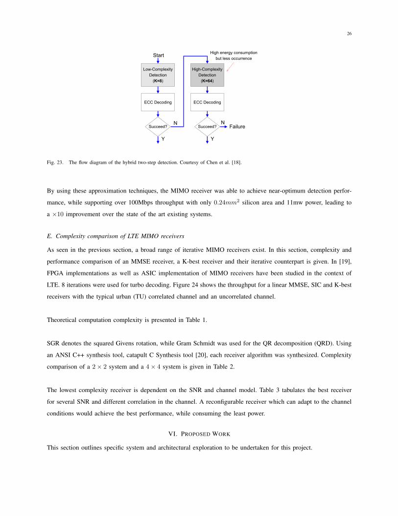
26

approach, the computational complexity can reduce to only about35% of a conventional K-best detector. Although the channel ma-trix decomposition has to be done twice, the cost can be marginalsince the channel is typically considered to be constant during thetransmission of several consecutive packets.

To evaluate the signal detection performance of the proposedbidirectional partial tree search approach, we performed computersimulations using the following system configurations that will alsobe used for all the other simulations throughout the paper: We con-sider LDPC-coded MIMO-OFDM system with 64-point FFT for4×4 MIMO transmission with 64-QAM. Out of the 64 subcarriers,48 are data carriers while the rest are used for pilots and virtualcarriers, as defined in the IEEE 802.11a standard. Each subcarrierMIMO channel remains constant during transmission of one packetand is subject to flat fading, i.e., all the entries in the MIMO channelmatrix are independent random Gaussian variables. Each packet isprotected by a length-2304, rate-1/2 LDPC code, where the LDPCcode decoder performs up to 15 decoding iterations. There is noiteration between MIMO detection and LDPC decoding. For thedefinition of the MIMO channel SNR, we follow the one proposedin [8]: Let R denote the channel code rate (R = 1 for uncodedsystems), SNR is defined as:

Eb

N0

˛˛dB

=Es

N0

˛˛dB

+ 10 log10Nr

R ·Nt · q,

where Es denotes the average symbol energy of the QAM con-stellation. As pointed out earlier, the radius r2 is calculated as2αNrσ

2 [8], where α = 6 is a predefined constant parameter andσ is the noise standard deviation. For the purpose of comparison,we also carried out simulations using depth-first sphere decodingalgorithm and conventional K-best detection scheme. The spheredecoder exhaustively examines all the paths that satisfy the sphereradius constraint for the calculation of the soft output. Therefore, itcan achieve better performance than the LSD scheme used in [6]that does not exhaustively examines all the paths satisfying thesphere radius constraint. All the detectors use the same radiusconstraint. As shown in Fig. 2, the K-best and bidirectional de-tectors have almost the same performance. Both of them have onlyvery small degradation compared to sphere decoder when K is large(e.g., 64). At very small value of K, the bidirectional K-best detec-tor is even slightly better than the conventional K-best detector.

15 15.5 16 16.5 17 17.5 18 18.5 1910-3

10-2

10-1

Eb/N

0(dB)

Pac

ket E

rror

Rat

e

Sphere DecodingK-Best (K=64)Bidirectional (K=64)K-Best (K=8)Bidirectional (K=8)

Figure 2: Simulated PER performance for 4×4 MIMO 64-QAM.

3.2 Hybrid Two-Step DetectionPractical wireless communication systems (such as IEEE 802.11n

and 3GPP LTE) typically target on achieving the packet error rate(PER) of 10−2 ∼ 10−3 at low SNR. Due to the significant impactof the value of K on the detection performance as shown in Fig. 2,we may need to use a large value of K (e.g., 64), which neverthelesstends to incur very high computational complexity. We note that,as shown in Fig. 2, although a small K (e.g., 8) will result in a bigSNR loss at the target detection PER, it still can achieve fair PERs(close to 10−1) in the low SNR range. This motivates us to pro-pose a hybrid two-step technique to reduce the average detectioncomputational complexity as described in the following. As shownin Fig. 3, in the first step, a simpler detector with K=8 is used. Ifthe ECC decoder fails to decode the packet correctly, all the vec-tors in the packet will be re-detected with K=64 in the second step.Therefore, majority of the packets can be successfully processedwith the simpler detector and only about 10% of packets need to befurther processed by the much more costly detector with K=64. Itshould be pointed out that, based on our computer simulations, theiterative detection/decoding scheme (i.e., feedback the soft-outputof the ECC decoder in the first step to the detection in the sec-ond step) fails to improve the overall system performance when thefirst-step detection is performed with very small K (e.g., 8). There-fore, we do not consider the use of iterative detection/decoding inthis work.

Low-ComplexityDetection

(K=8)

High-ComplexityDetection

(K=64)

ECC Decoding

Succeed?

Start

N

Y

ECC Decoding

Succeed?

Y

Failure

High energy consumptionbut less occurrence

N

Figure 3: The flow diagram of the hybrid two-step detection.

To further simplify the search for the admissible region duringthe path extension, we propose to use rectangular shaped admissi-ble region instead of the circular shaped admissible region in PSKenumeration technique. In the case of K=8, locating the admissi-ble points is very easy, especially when the bidirectional partial treesearch is used. Since each survivor only extend with k=K/2=4 mod-ulation points, we only need to find the 4 modulation points aroundPcli,i

at the i-th depth as shown in Fig. 4. For K=64, a rectangu-lar shaped region is formed by extending the inner 4-point squarewith the radius constraint as shown in Fig. 4. Although a few morepoints may be included in the rectangular shaped region than thecircular shaped region, it is much easier to define the boundaryand identify the admissible points. In the corresponding VLSI ar-chitecture design, the data flow will become very regular and thecontrol circuitry can be significantly simplified. Moreover, we pro-pose to realize path purge differently for K=8 and K=64: For K=8,we simply use the bubble sorter to select the best ones among allthe extended paths, while for K=64, we propose to use the memorybased-approximate sorter [4], as described in 2.3, in order to reducethe silicon area cost and power consumption.

Fig. 23. The flow diagram of the hybrid two-step detection. Courtesy of Chen et al. [18].

By using these approximation techniques, the MIMO receiver was able to achieve near-optimum detection perfor-

mance, while supporting over 100Mbps throughput with only 0.24mm2 silicon area and 11mw power, leading to

a ×10 improvement over the state of the art existing systems.

E. Complexity comparison of LTE MIMO receivers

As seen in the previous section, a broad range of iterative MIMO receivers exist. In this section, complexity and

performance comparison of an MMSE receiver, a K-best receiver and their iterative counterpart is given. In [19],

FPGA implementations as well as ASIC implementation of MIMO receivers have been studied in the context of

LTE. 8 iterations were used for turbo decoding. Figure 24 shows the throughput for a linear MMSE, SIC and K-best

receivers with the typical urban (TU) correlated channel and an uncorrelated channel.

Theoretical computation complexity is presented in Table 1.

SGR denotes the squared Givens rotation, while Gram Schmidt was used for the QR decomposition (QRD). Using

an ANSI C++ synthesis tool, catapult C Synthesis tool [20], each receiver algorithm was synthesized. Complexity

comparison of a 2× 2 system and a 4× 4 system is given in Table 2.

The lowest complexity receiver is dependent on the SNR and channel model. Table 3 tabulates the best receiver

for several SNR and different correlation in the channel. A reconfigurable receiver which can adapt to the channel

conditions would achieve the best performance, while consuming the least power.

VI. PROPOSED WORK

This section outlines specific system and architectural exploration to be undertaken for this project.

27KETONEN et al.: PERFORMANCE—COMPLEXITY COMPARISON OF RECEIVERS FOR A LTE MIMO–OFDM SYSTEM 3365

Fig. 7. Data transmission throughput versus SNR in a 2� 2 V-BLAST systemand moderately correlated channel.

The simplification has again only a small impact on the per-formance. Comparison of implementations done with the Cata-pult tool showed that the FPGA complexity is reduced approx-imately four times with the simplified LLR calculation. Alsothe SIC receiver is simplified from using soft demodulation forLLR calculation to using the approximate log-likelihood crite-rion. The symbol expectations are also calculated with (14).

IV. IMPLEMENTATION COMPARISONS

The theoretical complexity of the receivers with ispresented in Table III, where the number of multiplication, ad-dition, and comparison operations are specified. The memory isthe number of bits used in each block. In the squared Givens ro-tations (SGR) and the Gram–Schmidt based QRD, the divisionand square root were approximated with additions and shifts[28]. The term in the SGR comes from matrix multiplica-tions and in the QRD from multiple iterations of vector mul-tiplications. The number of operations in the -best algorithm

depends on the list size . If is larger than , it is usedas . In the first level , the number of multiplications isand additions . The LLR calculation operations for the linearreceivers depend on the modulation. The constant multiplica-tions with a power of 2 were calculated as shifts. The numberof multiplications is lower in the -best LSD than in the SICwith 4 4 QPSK. The number of multiplications in the -bestalgorithm increases with the list size and modulation. The mod-ulation order does not have a major impact on the complexitywith the SIC receiver. The impact of this can be seen later in theimplementation results. The SIC receiver includes more multi-plications than the -best algorithm with 4 4 QPSK and theimplementation gate count is also higher. With 64-QAM, thenumber of multiplications and gates is higher with the -best.

Catapult C Synthesis tool [29] was used in the implementa-tion of the receivers. It synthesizes algorithms written in ANSIC into high-performance, concurrent hardware. This singlesource methodology allows designers to pick the best archi-tecture for a given performance/area/power specification whileminimizing design errors and reducing the overall verification

Fig. 8. Data transmission throughput versus SNR in a 4� 4 system in (a) ahighly correlated, (b) moderately correlated, and (c) uncorrelated channel.

burden. While the results may not always be as optimal as withhand-coded HDL, the tool allows experimenting with differentarchitectures in a short amount of time and the comparisonof different algorithms can be made, provided they are imple-mented with the same tool. The complexity results seem to be

(a)

KETONEN et al.: PERFORMANCE—COMPLEXITY COMPARISON OF RECEIVERS FOR A LTE MIMO–OFDM SYSTEM 3365

Fig. 7. Data transmission throughput versus SNR in a 2� 2 V-BLAST systemand moderately correlated channel.

The simplification has again only a small impact on the per-formance. Comparison of implementations done with the Cata-pult tool showed that the FPGA complexity is reduced approx-imately four times with the simplified LLR calculation. Alsothe SIC receiver is simplified from using soft demodulation forLLR calculation to using the approximate log-likelihood crite-rion. The symbol expectations are also calculated with (14).

IV. IMPLEMENTATION COMPARISONS

The theoretical complexity of the receivers with ispresented in Table III, where the number of multiplication, ad-dition, and comparison operations are specified. The memory isthe number of bits used in each block. In the squared Givens ro-tations (SGR) and the Gram–Schmidt based QRD, the divisionand square root were approximated with additions and shifts[28]. The term in the SGR comes from matrix multiplica-tions and in the QRD from multiple iterations of vector mul-tiplications. The number of operations in the -best algorithm

depends on the list size . If is larger than , it is usedas . In the first level , the number of multiplications isand additions . The LLR calculation operations for the linearreceivers depend on the modulation. The constant multiplica-tions with a power of 2 were calculated as shifts. The numberof multiplications is lower in the -best LSD than in the SICwith 4 4 QPSK. The number of multiplications in the -bestalgorithm increases with the list size and modulation. The mod-ulation order does not have a major impact on the complexitywith the SIC receiver. The impact of this can be seen later in theimplementation results. The SIC receiver includes more multi-plications than the -best algorithm with 4 4 QPSK and theimplementation gate count is also higher. With 64-QAM, thenumber of multiplications and gates is higher with the -best.

Catapult C Synthesis tool [29] was used in the implementa-tion of the receivers. It synthesizes algorithms written in ANSIC into high-performance, concurrent hardware. This singlesource methodology allows designers to pick the best archi-tecture for a given performance/area/power specification whileminimizing design errors and reducing the overall verification

Fig. 8. Data transmission throughput versus SNR in a 4� 4 system in (a) ahighly correlated, (b) moderately correlated, and (c) uncorrelated channel.

burden. While the results may not always be as optimal as withhand-coded HDL, the tool allows experimenting with differentarchitectures in a short amount of time and the comparisonof different algorithms can be made, provided they are imple-mented with the same tool. The complexity results seem to be

(b)

Fig. 24. Throughput of MIMO receivers in (a) a typical urban correlated channel, and (b) an uncorrelated channel. Courtesy of Ketonen et al.

[19].

Table 1. The theoretical complexity of the receivers as numbers of arithmetic operations. Courtesy of Ketonen et al. [19].

3366 IEEE TRANSACTIONS ON SIGNAL PROCESSING, VOL. 58, NO. 6, JUNE 2010

TABLE IIITHE THEORETICAL COMPLEXITY OF THE RECEIVERS AS NUMBERS OF ARITHMETIC OPERATIONS

Fig. 9. Data transmission throughput versus SNR in a 2� 2 system in a highlycorrelated channel with the modified tree search.

Fig. 10. Data transmission throughput versus SNR in a 2� 2 system in a highlycorrelated channel with the simplified LLR calculation.

close to the hand-coded results with small designs. There canbe more difference with large designs.

The FPGA complexity results are presented in slices, 18-kbitBRAM and dedicated DSP slices. The DSP slices includean 18 18-bit multiplier. The VHDL from Catapult C wassynthesized to a Xilinx Virtex-4 FPGA with Mentor GraphicsPrecision Synthesis. The ASIC results are presented in gate

Fig. 11. The top-level architecture of the 2� 2�-best LSD.

equivalents (GE) and power consumption estimates. The Syn-opsys Design Compiler was used in synthesizing the VHDLalong with the UMC 0.18 m complementary metal oxidesemiconductor (CMOS) technology. The Synopsys Prime-Power was used for obtaining the statistical activity powerestimates for the implementations.

A. -Best LSD

The -best LSD receiver includes the QRD block, the-best LSD block and the LLR calculation block. The QR

decomposition block is based on the QRD algorithm from[30]. Ordering of the channel matrix is not utilized in thearchitecture. The top level architecture of the -best LSD fora 2 2 antenna system is shown in Fig. 11. The 4 4 antennasystem LSD is based on the same architecture but four morePED calculation blocks and sorters are added to the design.

The -best LSD architecture is modified from [20]. A 2 2and a 4 4 antenna system with a real signal model [31] isassumed. The received signal vector is multiplied with ma-trix in the matrix multiplication block. Matrix is mul-tiplied with the possible transmitted symbols after the QRDis performed, i.e., when the channel realization changes. Eu-clidean distances between the last symbol in vector and pos-sible transmitted symbols are calculated in block PED1 in a2 2 antenna system with . The resultinglists of symbols and Euclidean distances are not sorted at thefirst stage. The distances are added to the Euclidean distances

calculated in the PED2 block. Thelists are sorted and partial symbol vectors with the smallestEuclidean distances are kept. PED3 block calculates

which are added to the previousdistance and sorted. The last PED block calculates the partialEuclidean distances .After adding the previous distances to , the lists are sorted

28

Table 2. Complexity comparison of MIMO receivers in (a) a 2× 2, and (b) a 4× 4 system. Courtesy of Ketonen et al. [19].

3370 IEEE TRANSACTIONS ON SIGNAL PROCESSING, VOL. 58, NO. 6, JUNE 2010

TABLE XTHE PERFORMANCE-COMPLEXITY TRADEOFF WITH 2� 2 16-QAM AND

DETECTION RATE OF 140 MB/S

TABLE XITHE PERFORMANCE-COMPLEXITY TRADEOFF WITH 4� 4 16-QAM AND

DETECTION RATE OF 280 MB/S

). The goodput now encapsulates performances ofboth the implementation and the transmission.

The LMMSE receiver would require almost 10 dB moretransmit power in order to achieve the goodput of the -bestLSD but the complexity is much higher with the -best LSD.The SIC receiver does not achieve the goodput of the -bestLSD but has a much lower complexity. In the 4 4 antennacase, the SIC and LMMSE receivers do not give much goodputat lower SNRs but all the receivers have a high goodput whenthe SNR is high enough. If the channel is less correlated, thereceivers have a more similar performance and less transmitpower is needed to achieve a high goodput. The SIC receiverproduces the most bits per gate equivalent in the 2 2 antennasystem but at the 4 4 system, the -best LSD is the mostefficient. A part of the performance degradation of the SICreceiver in the 4 4 antenna system is due to the encoding ofthe streams in LTE, which leads to interference cancellationbeing performed between two layer pairs and the two layerpairs being separated only by the LMMSE equalizer. The SICreceiver would still provide a higher goodput than the LMMSEreceiver with a lower power consumption than the -bestLSD, thus offering a compromise between performance andcomplexity.

As a final illustration of the performance-complexity trade-off, the required transmit power to satisfy the rate and qualityrequirements is considered in a simple example case. The powerefficiency of the transmitter in transmit power/transmission ratein a 4 4 antenna system with a 20 MHz bandwidth is pre-sented in Fig. 16. The needed transmit power was obtained from

, where is the free space path lossis the receiver noise floor ( Receiver

noise figure of 6 dB) and FM is a 30-dB fade margin ( is thewavelength, is the distance from the base station, is Boltz-mann’s constant, is the temperature [K] and is the band-width). The SNR is the signal strength at the receiver requiredto achieve the maximum goodput. A simple path loss modelwithout shadowing or reflections was chosen for simplicity. Therequired transmit power of the LMMSE receiver is at least twiceof that of the -best LSD. The transmit energy per bit growswith the modulation order and is the same with 64-QAM -best

Fig. 16. The transmitter energy consumption per reliably transmitted bit versusthe propagation distance.

LSD and 16-QAM LMMSE. The -best LSD can receive datareliably from a higher distance than the SIC or LMMSE receiverwith a fixed transmit power. With 4 4 64-QAM, the LMMSEreceiver can receive data at only very short distances with a rea-sonable transmit power. Therefore, a more complex receiver isneeded to receive data from also larger distances.

Comparison of both performance and implementation toliterature can be difficult as the used channel models, methodsand the implementation technologies may be different. Manyof the implementations in the literature consider an uncodedsystem or an uncorrelated channel, where also simple receiversperform well, which can lead to different parameters in theimplementation. Depth-first sphere detector implementationsin the literature usually report an SNR dependent throughputwhich makes the implementation comparison more chal-lenging. The hard-output -norm -best detectors in [19] havea lower complexity but were implemented with different listsizes and CMOS technology from our work. The complexityof the receiver increases by roughly 30% both in [19] and thiswork when the list size is doubled. However, the detection ratedecreases almost five times in [19] but is only halved in ourwork. The soft output -best implementation in [12] with a listsize of 5 in a 4 4 16-QAM system has almost a three timeslower throughput and half the complexity of our implementa-tion with a list size 8. A soft output -best detector is presentedin [34]. It achieves a 50-Mb/s throughput with 4 4 64-QAM,list size 256 and a silicon area of 20 mm . The silicon area ofour implementation is four times smaller with the same CMOStechnology and the throughput is 210 Mb/s with a list size 16.

VI. CONCLUSION

The performances and implementation complexities of theLMMSE, SIC, noniterative and iterative -best LSD receiversfor MIMO–OFDM communications were compared. Theemphasis was on LTE specific system parameters and latencyrequirements. The SIC receiver was shown to outperform the

-best LSD with horizontal encoding in channels with lowspatial correlation, but the result is reversed in channels withsignificant spatial correlation; the SIC receiver is not practically

(a)

3370 IEEE TRANSACTIONS ON SIGNAL PROCESSING, VOL. 58, NO. 6, JUNE 2010

TABLE XTHE PERFORMANCE-COMPLEXITY TRADEOFF WITH 2� 2 16-QAM AND

DETECTION RATE OF 140 MB/S

TABLE XITHE PERFORMANCE-COMPLEXITY TRADEOFF WITH 4� 4 16-QAM AND

DETECTION RATE OF 280 MB/S

). The goodput now encapsulates performances ofboth the implementation and the transmission.

The LMMSE receiver would require almost 10 dB moretransmit power in order to achieve the goodput of the -bestLSD but the complexity is much higher with the -best LSD.The SIC receiver does not achieve the goodput of the -bestLSD but has a much lower complexity. In the 4 4 antennacase, the SIC and LMMSE receivers do not give much goodputat lower SNRs but all the receivers have a high goodput whenthe SNR is high enough. If the channel is less correlated, thereceivers have a more similar performance and less transmitpower is needed to achieve a high goodput. The SIC receiverproduces the most bits per gate equivalent in the 2 2 antennasystem but at the 4 4 system, the -best LSD is the mostefficient. A part of the performance degradation of the SICreceiver in the 4 4 antenna system is due to the encoding ofthe streams in LTE, which leads to interference cancellationbeing performed between two layer pairs and the two layerpairs being separated only by the LMMSE equalizer. The SICreceiver would still provide a higher goodput than the LMMSEreceiver with a lower power consumption than the -bestLSD, thus offering a compromise between performance andcomplexity.

As a final illustration of the performance-complexity trade-off, the required transmit power to satisfy the rate and qualityrequirements is considered in a simple example case. The powerefficiency of the transmitter in transmit power/transmission ratein a 4 4 antenna system with a 20 MHz bandwidth is pre-sented in Fig. 16. The needed transmit power was obtained from

, where is the free space path lossis the receiver noise floor ( Receiver

noise figure of 6 dB) and FM is a 30-dB fade margin ( is thewavelength, is the distance from the base station, is Boltz-mann’s constant, is the temperature [K] and is the band-width). The SNR is the signal strength at the receiver requiredto achieve the maximum goodput. A simple path loss modelwithout shadowing or reflections was chosen for simplicity. Therequired transmit power of the LMMSE receiver is at least twiceof that of the -best LSD. The transmit energy per bit growswith the modulation order and is the same with 64-QAM -best

Fig. 16. The transmitter energy consumption per reliably transmitted bit versusthe propagation distance.

LSD and 16-QAM LMMSE. The -best LSD can receive datareliably from a higher distance than the SIC or LMMSE receiverwith a fixed transmit power. With 4 4 64-QAM, the LMMSEreceiver can receive data at only very short distances with a rea-sonable transmit power. Therefore, a more complex receiver isneeded to receive data from also larger distances.

Comparison of both performance and implementation toliterature can be difficult as the used channel models, methodsand the implementation technologies may be different. Manyof the implementations in the literature consider an uncodedsystem or an uncorrelated channel, where also simple receiversperform well, which can lead to different parameters in theimplementation. Depth-first sphere detector implementationsin the literature usually report an SNR dependent throughputwhich makes the implementation comparison more chal-lenging. The hard-output -norm -best detectors in [19] havea lower complexity but were implemented with different listsizes and CMOS technology from our work. The complexityof the receiver increases by roughly 30% both in [19] and thiswork when the list size is doubled. However, the detection ratedecreases almost five times in [19] but is only halved in ourwork. The soft output -best implementation in [12] with a listsize of 5 in a 4 4 16-QAM system has almost a three timeslower throughput and half the complexity of our implementa-tion with a list size 8. A soft output -best detector is presentedin [34]. It achieves a 50-Mb/s throughput with 4 4 64-QAM,list size 256 and a silicon area of 20 mm . The silicon area ofour implementation is four times smaller with the same CMOStechnology and the throughput is 210 Mb/s with a list size 16.

VI. CONCLUSION

The performances and implementation complexities of theLMMSE, SIC, noniterative and iterative -best LSD receiversfor MIMO–OFDM communications were compared. Theemphasis was on LTE specific system parameters and latencyrequirements. The SIC receiver was shown to outperform the

-best LSD with horizontal encoding in channels with lowspatial correlation, but the result is reversed in channels withsignificant spatial correlation; the SIC receiver is not practically

(b)

Table 3. Receiver with the best goodput (QAM constellation). Courtesy of Ketonen et al. [19].

KETONEN et al.: PERFORMANCE—COMPLEXITY COMPARISON OF RECEIVERS FOR A LTE MIMO–OFDM SYSTEM 3371

TABLE XIITHE RECEIVER WITH THE BEST GOODPUT (QAM CONSTELLATION �)

suitable for vertically encoded MIMO communications. Softinformation feedback from the FEC decoder to the -bestLSD stage was also considered as a strategy to improve theperformance. It provides up to 2-dB performance improvement.The choice of the receiver algorithm is emphasized when thenumber of antennas increases and the channel condition numberis high. There the nonlinear ML or MAP based receivers clearlyoutperform the linear receivers, but the price is remarkablyincreased computational complexity.

The considered receivers were synthesized to a Xilinx FPGAto get a solid ground for implementation complexity compar-ison. A modification on the tree search of the -best LSD waspresented to simplify its implementation with no compromise inits error rate performance. Thus, it can achieve double detectionrate compared to the original -best algorithm. On the selectedFPGA, the SIC receiver is fast enough to process the numberof subcarriers defined in the LTE standard for 5-MHz band-width with all modulations and 2 2 and 4 4 antenna con-figurations. ASIC implementation results were also provided.The receivers were designed to have the same detection rate,which would be enough for the LTE 20-MHz bandwidth. The

-best LSD was found to be more than twice as complex as theSIC receiver in the 2 2 antenna case but in the 4 4 case thecomplexity difference was smaller. The latency of the SIC re-ceiver does not depend on the used modulation and it can be usedwith higher order modulations. The latency of the -best LSDincreases with the modulation and the list size in both FPGAand ASIC implementations. The maximum detection rates inthe ASIC implementations were 420 Mb/s with the SIC receiverand 280 Mb/s with the -best LSD.

The receivers with the highest goodput and the lowestcomplexity on ASIC with correlated, moderately correlatedand uncorrelated channels with a given SNR are presented inTable XII. It can be seen that the simpler LMMSE and SICreceivers can be used in the uncorrelated channel but in thecorrelated channel, the -best LSD gives the best goodput. Thereceiver and the modulation order could be changed adaptivelywith the channel conditions and SNR in order to achieve thebest possible goodput with the least amount of receive power.

Some open research problems still remain. The system westudied assumed that there is no channel state information atthe transmitter. With full or partial transmitter channel stateinformation, low mobility appropriate feedback schemes com-bined with transmitter precoding could change the conclusionsand would be an interesting line of further work. Also addingchannel estimation to the performance and complexity eval-

uation would be an interesting topic. One further promisingtopic would be the design and implementation of a reconfig-urable overall architecture which would adaptively switch usinga simple or a more complex detector depending on the transmis-sion requirements, available SNR, channel properties, etc. Somepreliminary results for the study of receivers for adaptive mod-ulation and coding can be found in [35].

ACKNOWLEDGMENT

The authors would like to thank Mentor Graphics for the pos-sibility to evaluate Catapult C Synthesis tool and M. Myllylä andJ. Ylioinas for their helpful comments.

REFERENCES

[1] H. Boelcskei, “MIMO-OFDM wireless systems: Basics, perspectives,and challenges,” IEEE Trans. Commun., vol. 13, no. 4, pp. 31–37, Aug.2006.

[2] H. Artes, D. Seethaler, and F. Hlawarsch, “Efficient detection algo-rithms for MIMO channels: A geometrical approach to approximateML detection,” IEEE Trans. Signal Process., vol. 51, no. 11, pp.2808–2820, Nov. 2003.

[3] G. J. Foschini and M. J. Gans, “On limits of wireless communicationsin a fading environment when using multiple antennas,” in WirelessPers. Commun.. : Kluwer, 1998, vol. 6, pp. 311–335.

[4] P. W. Wolniansky, G. J. Foschini, G. D. Golden, and R. A. Valenzuela,“V-BLAST: An architecture for realizing very high data rates over therich-scattering wireless channel,” in Proc. Int. Symp. Signals, Systems,Electronics (ISSSE), Pisa, Italy, Sept. 29–Oct. 2 1998, pp. 295–300.

[5] G. D. Golden, C. J. Foschini, R. A. Valenzuela, and P. W. Wolniansky,“Detection algorithm and initial laboratory results using V-BLASTspace-time communication architecture,” IEE Electron. Lett., vol. 35,no. 1, pp. 14–16, Jan. 1999.

[6] X. Wautelet, A. Dejonghe, and L. Vandendorpe, “MMSE-based frac-tional turbo receiver for space-time BICM over frequency-selectiveMIMO fading channels,” IEEE Trans. Signal Process., vol. 52, no. 6,pp. 1804–1809, Jun. 2004.

[7] M. Sellathurai and S. Haykin, “TURBO-BLAST for wireless commu-nications: Theory and experiments,” IEEE Trans. Signal Process., vol.50, no. 10, pp. 2538–2546, Oct. 2002.

[8] M. O. Damen, H. El Gamal, and G. Caire, “On maximum–likelihooddetection and the search for the closest lattice point,” IEEE Trans. Inf.Theory, vol. 49, no. 10, pp. 2389–2402, Oct. 2003.

[9] U. Fincke and M. Pohst, “Improved methods for calculating vectorsof short length in a lattice, including a complexity analysis,” Math.Comput., vol. 44, no. 5, pp. 463–471, May 1985.

[10] B. Hochwald and S. ten Brink, “Achieving near-capacity on a multiple-antenna channel,” IEEE Trans. Commun., vol. 51, no. 3, pp. 389–399,Mar. 2003.

[11] K. Wong, C. Tsui, R. K. Cheng, and W. Mow, “A VLSI architectureof a K-best lattice decoding algorithm for MIMO channels,” in Proc.IEEE Int. Symp. Circuits Systems, Scottsdale, AZ, May 26–29, 2002,vol. 3, pp. 273–276.

[12] Z. Guo and P. Nilsson, “Algorithm and implementation of the K-bestsphere decoding for MIMO detection,” IEEE J. Sel. Areas Commun.,vol. 24, no. 3, pp. 491–503, Mar. 2006.

[13] C. Studer, A. Burg, and H. Bolcskei, “Soft-output sphere decoding:Algorithms and VLSI implementation,” IEEE J. Sel. Areas Commun.,vol. 26, no. 2, pp. 290–300, Feb. 2008.

[14] M. Myllylä, M. Juntti, and J. R. Cavallaro, “Architecture design andimplementation of the increasing radius—List sphere detector algo-rithm,” in Proc. IEEE Int. Conf. Acoust., Speech, Signal Processing,Taipei, Taiwan, Apr. 2009, pp. 553–556.

[15] P. Bhagawat, R. Dash, and G. Choi, “Systolic like soft-detection archi-tecture for 4� 4 64-QAM MIMO system,” in Proc. Design, Automa-tion Test in Eur. Conf. Exhibit., Nice, France, Apr. 2009, pp. 870–873.

[16] S. Mondal, A. M. Eltawil, and K. N. Salama, “Architectural opti-mizations for low-power K-best MIMO decoders,” IEEE Trans. Veh.Technol., vol. 58, no. 7, pp. 3145–3153, Sep. 2009.

[17] J. Antikainen, P. Salmela, O. Silvén, M. Juntti, J. Takala, and M. Myl-lylä, “Fine-grained application-specific instruction set processor designfor the�-best list sphere detector algorithm,” in Proc. Int. Symp. Sys-tems, Architectures, Modeling, Simulation (SAMOS), Samos, Greece,Jul. 21–24, 2008, pp. 108–115.

A. Turbo scheduling

Turbo MIMO receivers consisting of an inner turbo decoder loop and an outer loop between a SISO MIMO detector

and the turbo decoder, offers the possibility of BER-optimally allocating the number of iterations between the two

loops given a fixed iteration budget. For an iterative turbo MIMO receiver, where the channel decoder itself is also

iterative (as in turbo or LDPC code), it is not clear whether it is beneficial to run the iterative channel decoder till it

converges then feed back the information to the MIMO detector. For better BER performance, it is possible that just

performing a few iterations to get slightly better priors for the soft MIMO detector can improve the performance

significantly. Such scheduling can also reduce the complexity/power of the iterative decoder significantly. One

analytical method to create such an optimized scheduling can be the use of an EXIT (extrinsic information transfer)

chart. By having, possibly, a three dimensional EXIT chart (between the iterative parts of the channel decoder, and

the MIMO detector), a BER and power-optimal scheduling strategy will be explored.

B. Receiver algorithm development

After considering the average and worst case computational complexities of current state of the art receiver

algorithms, we will focus on developing a new receiver structure. Current work that has been done on turbo MIMO

receivers can be categorized as developing a new soft MIMO detector and pairing it with a channel code such as

a convolutional code or turbo code. Soft detectors have been developed for the widely existing hard detectors, and

a mix and match scheme has been used to implement each block of the fundamental architecture of iterative turbo

MIMO receiver. Thus, by developing a new soft MIMO detection algorithm, a new class of iterative receiver can

be created which can generate many different receivers based on the channel decoder type.

29

One example of such nascent detector is the Markov chain Monte Carlo (MCMC) [21] based MIMO detection.

Computing the soft information based on all possible transmit symbols is a prohibitively expensive task. The main

idea of the MCMC is to use Gibbs sampling to find a list of most likely pairs of transmitted sequence and then

compute the soft information. The complexity of the MCMC will be dependent on the list size.

C. Architectural exploration of turbo MIMO receivers

Though there has been much work done on algorithmic exploration of iterative MIMO receivers, its implementation

aspect has lacked attention. For one, the effect of implementation precision and quantization on the LLR calculation

and overall power/performance tradeoff is yet to be explored.

Optimization of the iterative framework can also be explored. Much work has been done on the architecture of the

components of an iterative MIMO receiver. Turbo decoders, turbo equalizers, MIMO detector architectures have

all been studied as stand-alone blocks. Optimization of these existing blocks in the context of an iterative MIMO

receiver will be beneficial as the work done on existing blocks can be utilized and leveraged. On the other hand, in

the context of an iterative receiver, the implementation of the component blocks could differ considerably. Being

aware of such soft information exchange could simplify the MIMO detector or channel decoder architecture. Once

the iterative system and its components are optimized independently, it is also natural to consider joint optimization

of the whole system.

In addition to the above, we could make use of the many common computational kernels between various soft

MIMO detectors to develop an application specific instruction processor (ASIP) tailored for soft MIMO detection.

Examples of such kernels include: matrix multiplication and QR decomposition in the preprocessing stage and LLR

computation in the output stage. Commercially available ASIP design tools such as Target (www.retarget.com) or

Coware (part of Synopsis) will be employed in this exploration.

REFERENCES

[1] P. Wolniansky, G. Foschini, G. Golden, and R. Valenzuela, “V-blast: an architecture for realizing very high data rates over the rich-scattering

wireless channel,” in Signals, Systems, and Electronics, 1998. ISSSE 98. 1998 URSI International Symposium on, Sep. 1998, pp. 295 –300.

[2] R. Kannan, “Improved algorithms for integer programming and related lattice problems,” in Proceedings of the fifteenth annual ACM

symposium on Theory of computing. ACM, 1983, pp. 193–206.

[3] J. Lagarias, H. Lenstra, and C. Schnorr, “Korkin-Zolotarev bases and successive minima of a lattice and its reciprocal lattice,” Combinatorica,

vol. 10, no. 4, pp. 333–348, 1990.

[4] U. Fincke and M. Pohst, “Improved methods for calculating vectors of short length in a lattice, including a complexity analysis,” Mathematics

of computation, pp. 463–471, 1985.

[5] Z. Guo and P. Nilsson, “VLSI implementation issues of lattice decoders for MIMO systems,” in Proc. IEEE ISCAS, May 2004, pp. IV –

477–480.

[6] W.-J. Choi, R. Negi, and J. Cioffi, “Combined ML and DFE decoding for the V-BLAST system,” in Communications, 2000. ICC 2000.

2000 IEEE International Conference on, vol. 3, 2000, pp. 1243 –1248 vol.3.

30

[7] J. W. Choi, B. Shim, A. Singer, and N. I. Cho, “Low-complexity decoding via reduced dimension maximum-likelihood search,” IEEE

Transactions on Signal Processing, vol. 58, no. 3, pp. 1780–1793, Mar. 2010.

[8] C. Berrou and A. Glavieux, “Near optimum error correcting coding and decoding: Turbo-codes,” IEEE Transactions on Communications,

vol. 44, no. 10, pp. 1261 –1271, Oct. 1996.

[9] B. Hochwald and S. ten Brink, “Achieving near-capacity on a multiple-antenna channel,” IEEE Transactions on Communications, vol. 51,

no. 3, pp. 389 – 399, Mar. 2003.

[10] C. Studer, A. Burg, and H. Bolcskei, “Soft-output sphere decoding: algorithms and VLSI implementation,” IEEE Journal on Selected

Areas in Communications, vol. 26, no. 2, pp. 290 –300, Feb. 2008.

[11] M. Sellathurai and S. Haykin, “Turbo-BLAST for wireless communications: theory and experiments,” IEEE Transactions on Signal

Processing, vol. 50, no. 10, pp. 2538–2546, 2002.

[12] C. Berrou, A. Glavieux, and P. Thitimajshima, “Near Shannon limit error-correcting coding and decoding: Turbo-codes,” in IEEE

International conference on Communications (ICC), vol. 2. IEEE, 1993, pp. 1064–1070.

[13] C. Douillard, M. Jezequel, C. Berrou et al., “Iterative correction of intersymbol interference: Turbo-equalization,” European Transactions

on Telecommunications, vol. 6, no. 5, pp. 507–511, 1995.

[14] D. Zuyderhoff, X. Wautelet, A. Dejonghe, and L. Vandendorpe, “MMSE turbo receiver for space-frequency bit-interleaved coded OFDM,”

in IEEE 58th Vehicular Technology Conference, vol. 1. IEEE, 2003, pp. 567–571.

[15] J. Wang and S. Li, “MIMO turbo receiver with new probability data association soft interference cancellation,” in International Conference

on Communications, Circuits and Systems, vol. 1. IEEE, pp. 232–236.

[16] H. Vikalo, B. Hassibi, and T. Kailath, “Iterative decoding for MIMO channels via modified sphere decoding,” IEEE Transactions on

Wireless Communications, vol. 3, no. 6, pp. 2299–2311, 2004.

[17] Y. de Jong and T. Willink, “Iterative tree search detection for MIMO wireless systems,” IEEE Transactions on Communications, vol. 53,

no. 6, pp. 930–935, 2005.

[18] S. Chen and T. Zhang, “Low power soft-output signal detector design for wireless MIMO communication systems,” in Proc. IEEE ISLPED,

2007, pp. 232–237.

[19] J. Ketonen, M. Juntti, and J. Cavallaro, “Performance-complexity comparison of receivers for a LTE MIMO–OFDM system,” IEEE

Transactions on Signal Processing, vol. 58, no. 6, pp. 3360–3372, 2010.

[20] “Catapult C synthesis datasheet,” Mentor Graphics, Datasheet, 2008.

[21] B. Farhang-Boroujeny, H. Zhu, and Z. Shi, “Markov chain Monte Carlo algorithms for CDMA and MIMO communication systems,” IEEE

Transactions on Signal Processing, vol. 54, no. 5, pp. 1896–1909, 2006.