1. fundamentals of fluid dynamics
TRANSCRIPT
1. Fundamentals of Fluid Dynamics
1.1 Introduction
As pointed out in the Preface, the major thrust of this text is to extend ourdiscussion of spectral methods from the simple model problems and single-domain methods described in the companion book, CHQZ2, to practical ap-plications in fluid dynamics and to methods for complex domains. We referthe reader to Chap. 8 for a short introduction to spectral methods.
As preparation for the applications that are the focus of Chaps. 2–4, inthis chapter we provide a survey of the fundamentals of fluid dynamics. Webegin with some general background material on fluids on fluids, then con-centrate on the basic equations of fluid dynamics (in Eulerian form). Theseequations are first stated in their full generality for compressible flow. Sub-sequent expositions include various special cases, especially those to whichspectral methods have most commonly been applied. These special casesinclude Euler equations, incompressible Navier–Stokes equations, boundary-layer equations, and equations for both linear and nonlinear stability analysis.We also include some historical background on the various systems of equa-tions that have been used over the years in the study of fluid dynamics.
The reader interested in detailed derivations and physical interpretationsof these equations should consult standard references such as Courant andFriedrichs (1976), Howarth (1953), Liepmann and Roshko (2001), Landau andLifshitz (1987), Serrin (1959a), Moore (1989), Batchelor (2000), Schlichtingand Gersten (1999), and the various texts on more specialized topics citedbelow. (Most of these texts have been published in several editions. We havelisted them here in the chronological order of their first editions but providea reference to the most recent edition as of the publication of this text; weuse this convention for ordering references throughout this book.)
1.2 Fluid Dynamics Background
Gases, such as air, and liquids, such as water, are both fluids. Before pro-ceeding to the partial differential equations that describe the motion of suchfluids, we provide the basis for the distinction between these two types offluids and then summarize the relevant thermodynamic relationships.
2 1. Fluid Dynamics
1.2.1 Phases of Matter
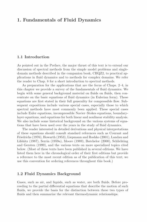
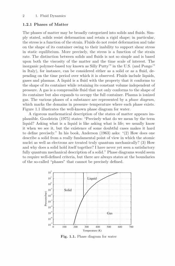
The phases of matter may be broadly categorized into solids and fluids. Sim-ply stated, solids resist deformation and retain a rigid shape; in particular,the stress is a function of the strain. Fluids do not resist deformation and takeon the shape of its container owing to their inability to support shear stressin static equilibrium. More precisely, the stress is a function of the strainrate. The distinction between solids and fluids is not so simple and is basedupon both the viscosity of the matter and the time scale of interest. Theinorganic polymer-based toy known as Silly Putty™ in the U.S. (and Pongo™in Italy), for instance, can be considered either as a solid or as a fluid, de-pending on the time period over which it is observed. Fluids include liquids,gases and plasmas. A liquid is a fluid with the property that it conforms tothe shape of its container while retaining its constant volume independent ofpressure. A gas is a compressible fluid that not only conforms to the shape ofits container but also expands to occupy the full container. Plasma is ionizedgas. The various phases of a substance are represented by a phase diagram,which marks the domains in pressure–temperature where each phase exists.Figure 1.1 illustrates the well-known phase diagram for water.
A rigorous mathematical description of the states of matter appears im-plausible. Goodstein (1975) states: “Precisely what do we mean by the termliquid? Asking what is a liquid is like asking what is life; we usually knowit when we see it, but the existence of some doubtful cases makes it hardto define precisely.” In his book, Anderson (1963) asks: “(2) How does onedescribe a solid from a really fundamental point of view in which the atomicnuclei as well as electrons are treated truly quantum mechanically? (3) Howand why does a solid hold itself together? I have never yet seen a satisfactoryfully quantum mechanical description of a solid.” Phase diagrams would seemto require well-defined criteria, but there are always states at the boundariesof the so-called “phases” that cannot be precisely defined.
Fig. 1.1. Phase diagram for water
1.2 Fluid Dynamics Background 3
To be extremely precise, one should speak of “fluid-like” and “solid-like”behavior; their distinction depends upon the time and the length scales ofinterest. Glaciers and the Earth’s mantle flow are thus fluid-like if the timescale is appropriately large, while they can be considered as solids if the timescale is appropriately small. However, it is not merely a matter of the timescale. Even if the time scale is on the order of months and the length scaleon the order of miles, the Earth’s mantle can be modeled as a solid, while ifthe length scale is the order of nanometers or less it may be appropriate tomodel it as a fluid. This suggests the need for appropriate nondimensionalnumbers. In rational mechanics, the nondimensional Deborah number (seeHuilgol (1975)) is the ratio of a process time to an inherent relaxation time.The same lump of borosiloxane can be observed to flow as a fluid if the timescale is sufficiently large, to deform like an elastic solid, or to shatter likebrittle glass.
Perhaps, the most accurate and lucid discussion of the distinction be-tween solid-like and fluid-like behavior was given by Maxwell (1872): “Whatis required to alter the form of a soft solid is a sufficient force, and, this whenapplied produces its effect at once. In the case of viscous fluid it is time thatis required, and if enough time is given, the very smallest force will producea sensible effect, such as would require a very large force if suddenly applied.Thus a block of pitch may be so hard that you cannot make a dent in itby striking it with your knuckles; and yet it will in course of time, flattenitself by its own weight, and glide down hill like a stream of water.” Maxwellis clearly referring to the importance of time scales and to a material thatseems to have two time scales. However, materials can have more than twotime scales.
1.2.2 Thermodynamic Relationships
General Gases. A complete description of a single-phase, homogeneous fluidis available if, as a function of space and time, the velocity u = (u, v, w)T ,any two thermodynamic variables, and an equation of state are known. (Thesuperscript T denotes the transpose of a vector or matrix.). The basic ther-modynamic variables of most interest in fluid dynamics are the density ρ (orspecific volume V = 1/ρ), the pressure p, the temperature T , the specificinternal energy e, the specific entropy s, and the specific enthalpy h. (A spe-cific quantity is one per unit mass.) Of these state variables, only two areindependent, and the others can be expressed as functions of the two inde-pendent variables. In the classical Gibbs axiomatic formulation, the equationof state is
e = e(V, s) , (1.2.1)
and the variables pressure and temperature are defined by
p = − ∂e∂V
and T =∂e
∂s, (1.2.2)
4 1. Fluid Dynamics
respectively, where p and T are always positive. By forming the total differ-ential of the relation e = e(V, s), we obtain the fundamental thermodynamicrelation
T ds = de+ p dV . (1.2.3)
This may be considered a corollary of the second law of thermodynamics,and it defines the specific entropy, denoted by s.
The (specific) total energy is defined as
E = e+12(u · u) , (1.2.4)
the (specific) enthalpy is defined as
h = e+ p/ρ , (1.2.5)
and the (specific) total enthalpy is defined as
H = h+12(u · u) . (1.2.6)
The various relations among p, V , T , e, and s are known as equations ofstate. Relations giving p as a function of ρ (or V ) and s (or T ) occur withthe greatest frequency in the theory of fluids:
p = f1(ρ, T ) or p = f2(V, s) or p = f3(ρ, s) . (1.2.7)
Such relations are usually referred to as caloric equations of state. A unit massof fluid in thermodynamic equilibrium has two important heat capacities
Cv = T∂s
∂T
∣∣∣∣V
and Cp = T∂s
∂T
∣∣∣∣p
. (1.2.8)
They are called, respectively, the specific heat at constant volume and thespecific heat at constant pressure. Experimental observations support the as-sumption that both specific heats are always positive. Using (1.2.3) and thecorresponding total differential of the enthalpy, one obtains
Cv =∂e
∂T
∣∣∣∣V
and Cp =∂h
∂T
∣∣∣∣p
. (1.2.9)
From (1.2.3) and the first part of (1.2.9), we have
Cp − Cv =(
p+∂e
∂V
∣∣∣∣T
)∂V
∂T
∣∣∣∣p
. (1.2.10)
Differentiating (1.2.3) with respect to T and V , respectively, we have
∂s
∂T
∣∣∣∣V
=1T
∂e
∂T
∣∣∣∣V
,∂s
∂V
∣∣∣∣T
=1T
(
p+∂e
∂V
∣∣∣∣T
)
. (1.2.11)
1.2 Fluid Dynamics Background 5
Then, equating the derivative of the former with respect to V with the deriva-tive of the latter with respect to T , we have
p+∂e
∂V
∣∣∣∣T
=∂p
∂T
∣∣∣∣V
. (1.2.12)
Hence, using (1.2.12) in (1.2.10), we have for the difference between the spe-cific heats:
Cp − Cv = − Tρ2
∂p
∂T
∣∣∣∣ρ
∂ρ
∂T
∣∣∣∣p
. (1.2.13)
(See Howarth (1953) for more details.)Another important positive quantity is
c2 =∂p
∂ρ
∣∣∣∣s
, (1.2.14)
where c is called the sound speed , which is the speed at which sound wavestravel in the fluid (see Sect. 4.3).
Perfect Gases. The preceding equations are the general thermodynamic re-lationships. A number of special cases are of practical interest. A thermallyperfect gas (also known as an ideal gas) is a fluid that obeys Boyle’s Law,which is expressed by the equation of state
p = ρRT , (1.2.15)
where the gas constant R is the ratio of the universal gas constant to theeffective molecular weight of the particular gas.
In many applications the fluid is assumed to be calorically perfect inaddition to being thermally perfect. For a thermally perfect gas one can showthat both the specific internal energy and the specific enthalpy are functionsof temperature only:
de = Cv(T )dT and dh = Cp(T )dT . (1.2.16)
A thermally perfect gas is called calorically perfect if the specific heatsare independent of temperature:
e = CvT and h = CpT , (1.2.17)
assuming of course that both e and h vanish if T vanishes. Equations (1.2.4)and (1.2.6) become, respectively,
E = CvT +12(u · u) (1.2.18)
andH = CpT +
12(u · u) . (1.2.19)

6 1. Fluid Dynamics
It can be proven that an ideal gas that is calorically perfect has the polytropicequation of state
p = f(ρ, s) = Kργ , (1.2.20)
where K depends on the entropy only and γ (called the adiabatic expo-nent) is the ratio of the specific heats, Cp/Cv. Its value lies in the interval1 < γ < 5/3 for most fluids, and it is usually assumed to be 1.4 for air atmoderate temperatures (< 800 ◦K).
For a calorically perfect gas (1.2.14) becomes
c2 =γp
ρ, (1.2.21)
and (1.2.13) reduces toCp − Cv = R . (1.2.22)
The latter equation leads to the relations
Cp =γ
γ − 1R and Cv =
1γ − 1
R , (1.2.23)
and the calorically perfect gas equation of state
p =ρe
γ − 1. (1.2.24)
Furthermore, we have that
γ =Cp
Cv. (1.2.25)
1.2.3 Historical Perspective
Before commencing our summary of the basic equations of fluid dynamics,we provide a brief historical perspective on the evolution of the mathemat-ical description of fluid motion. Navier (1827) must be credited with thefirst attempt at deriving the equations for homogeneous incompressible vis-cous fluids on the basis of considerations involving the action of intermolec-ular forces. Poisson (1831) derived the equations for compressible fluids froma similar molecular model. The first mathematical description of the motionof an “ideal” (inviscid and incompressible) fluid was, however, due to Euler(1755), who applied Newton’s second law of motion to a fluid moving underan internal force known as the pressure gradient. D’Alembert (1752) was thefirst to point out that this mathematical model leads to the eponymous para-dox that a body at rest in a uniform stream of ideal fluid suffers no drag:“a singular paradox which I leave to geometricians to explain”. AlthoughNavier’s (1827) intermolecular interaction model did include a viscous term,which was proportional to the Laplacian of the velocity field, he did notrecognize the physical significance of viscosity and considered the viscosity

1.3 Compressible Fluid Dynamics Equations 7
coefficient to be a function of molecular spacing. The continuum derivation ofthe Navier–Stokes equations is due to Saint-Venant (1843) and Stokes (1845).Saint-Venant published a derivation of the equations on a more physical ba-sis that applied not only to the so-called laminar flows considered by Navierbut also to turbulent flows. However, it was Stokes who, under the sole as-sumption that the stresses are linear functions of the strain rates, derivedthe equations in the form that is currently in use. Interesting details of thehistory of fluid dynamics can be found in Truesdell (1953), Darrigol (2002),and in the texts by Rouse and Ince (1963) and Grattan-Guinness (1990).
As noted above, Euler (1755) was the first to provide a mathematical de-scription of the motion of inviscid fluids. The Euler equations are often usedto simulate vortical flows such as those resulting from shocks or breakawayseparations whose basic mechanisms are not dominated by viscous effects.The matched asymptotic expansion theories (van Dyke (1975), Moore (1989))have established the relevance of the Euler solution as the first term of theouter expansion to be matched with the first term of the inner expansion,which describes the relatively thin boundary layer abutting the solid stream-lined boundary. Thus, the Euler solution coupled with corrections from theboundary-layer equations are sometimes used as an alternative to solving therelatively expensive full Navier–Stokes equations.
Prototypes of the concept of a boundary layer associated with the no-slip condition on a solid body had existed since the derivation of the equa-tions of motion of a viscous fluid (Stokes (1845), Rankine (1864), Froude(1872), Lorenz (1881)). However, it was Prandtl (1904) who first derivedwhat are now known as the boundary-layer equations based on the dimen-sional argument that in the thin layer adjacent to a body in a stream, theviscous stress in the streamwise direction is much larger than the normalstress and is of the same order of magnitude as the streamwise inertial force.The formal mathematical basis for deriving the boundary-layer theory fromthe Navier–Stokes equations was achieved by Lagerstrom and associates (seevan Dyke (1969)), who developed the singular perturbation theory or methodof matched asymptotic expansions. Simply stated, this consists of construct-ing the so-called outer and inner expansions by iterating the Navier–Stokesequations between an outer inviscid solution (that does not satisfy the no-slipcondition on the body) and an inner solution (that satisfies the no-slip condi-tion on the body) and matching them in their overlapping region of validity.Tani (1977) provides an excellent historical perspective on boundary-layertheory.
1.3 Compressible Fluid Dynamics Equations
This section begins with the most general form of the fluid dynamics equa-tions considered in this text, namely, the compressible Navier–Stokes equa-tions. Then various special or limiting forms of the compressible equations
8 1. Fluid Dynamics
are presented. The following section focuses on the incompressible versionsof these equations.
1.3.1 Compressible Navier–Stokes Equations
The constitutive equations are essential to the description of a viscous fluid.These are equations that relate the viscous stress tensor τ at a given pointx = (x, y, z) of the medium to the strain tensor S at that point. The termStokesian fluid is used for fluids that satisfy the conditions that the stresstensor (i) is a continuous function of the strain tensor (and independent ofall other kinematic quantities), (ii) is spatially homogeneous, (iii) is spatiallyisotropic, and (iv) is equal to −pI (where I is the unit tensor and p isa scalar) if the strain vanishes. These imply (see, e. g., Serrin (1959a)), thatthe stress tensor is a linear combination of the identity matrix, the straintensor, and the square of the strain tensor. Classical fluids are those forwhich the additional condition that the stress tensor is a linear function ofthe strain tensor is imposed. (The term Newtonian fluid is sometimes usedfor classical fluids, although this term is more properly applied to just theincompressible situation.) This yields the classical constitutive equation forthe total stress tensor σ:
σ = −pI + τ , (1.3.1)
with the viscous stress tensor
τ = 2μS + λ(∇ · u)I , (1.3.2)
and the strain-rate tensor
S =12[∇u + (∇u)T ] . (1.3.3)
Here, μ and λ are called the first and second coefficients of viscosity, respec-tively. The first coefficient of viscosity μ is also called the shear viscosity andoften simply the viscosity. The symbols ∇· and ∇ denote the divergence andgradient operators, respectively, with respect to the spatial coordinate x.
The viscous dissipation function Φ, which represents the work done bythe viscous stresses on a particle, is defined as
Φ = τ : ∇u , (1.3.4)
with the colon denoting the contraction of the double-index tensors. Theconstraint that the dissipation function is always nonnegative requires that
μ ≥ 0 and(
λ+23μ
)
≥ 0 . (1.3.5)
The expression (λ + 23μ) is called the bulk viscosity. The limiting case cor-
responding to μ = λ = 0 yields a simplified model, the Euler equations,discussed in Sect. 1.3.4.
1.3 Compressible Fluid Dynamics Equations 9
When the effect of thermal conduction is significant, one uses the Fourierlaw
q = −κ∇T (1.3.6)
to express the heat flux q as a function of the temperature gradient throughthe thermal conductivity κ.
The relationship between κ and μ is customarily written in terms of thePrandtl number , defined as
Pr =Cpμ
κ. (1.3.7)
This is the nondimensional ratio of the viscous diffusion to the thermal con-ductivity. The length scale for viscous diffusion is greater than or less thanthe length scale for thermal conductivity depending upon whether Pr is lessthan or greater than 1, respectively. In general, the Prandtl number is notconstant, although the simplifying assumption of a constant Prandtl numberis very common in applications.
The coefficients of viscosity and the thermal conductivity are dependentupon the thermodynamic variables, primarily the temperature. For gases, theshear viscosity is commonly taken from Sutherland’s formula
μ
μr=Tr + S1
T + S1
(T
Tr
)3/2
, (1.3.8)
where μr is the viscosity at the reference temperature Tr, S1 is a constant, andthe temperature T is given in degrees Kelvin. For air, S1 = 110.4 ◦K, and forthe reference values Tr = 273.1 ◦K and μr = 1.716× 10⁻⁴ gm/cm-sec, (1.3.8)becomes
μ =1.458 T 3/2
T + 110.4× 10⁻⁵ gm/cm-sec , (1.3.9)
and the bulk viscosity is taken to be zero, yielding
λ = −23μ . (1.3.10)
The algebraic form of Sutherland’s formula is based on molecular forces con-siderations (Sutherland (1893)), and the constants are determined by fittingexperimental data for a given gas (Anon. (1949, 1953)); for air, it is quiteaccurate for temperatures between 100 ◦K and 1890 ◦K. Although empiricalformulas for the thermal conductivity are also available, κ is often just takento be proportional to μ, i. e., the Prandtl number Pr is taken to be strictlyconstant in (1.3.7). For example, Pr = 0.7 is usually used for air.
The Navier–Stokes equations are a differential form of the three conser-vation laws that govern the motion in time t of classical fluids. The conserva-tion laws are first expressed in integral form as the appropriate conservationstatement for any arbitrary volume that moves with the fluid, accounting for
10 1. Fluid Dynamics
any relevant surface effects. The partial differential equations then follow un-der suitable continuity and differentiability conditions. The equation of massconservation, known as the continuity equation, is
∂ρ
∂t+ ∇ · (ρu) = 0 . (1.3.11)
The equation for momentum conservation is
∂(ρu)∂t
+ ∇ · (ρuuT ) + ∇p = ∇ · τ , (1.3.12)
and the equation for total energy conservation is
∂(ρE)∂t
+ ∇ · (ρEu) + ∇ · (pu) = −∇ · q + ∇ · (τu) . (1.3.13)
(In (1.3.12) the divergence of a tensor appears. The symbol ∇ · τ indicatesthe vector whose components are (∇ · τ )i =
∑
j∂τij
∂xj.) The momentum con-
servation statement that leads to (1.3.12) utilizes Newton’s second law viathe Cauchy principle that allows one to express the surface forces in terms ofthe total stress (volumetric forces have been neglected). The Navier–Stokesequations (1.3.11)–(1.3.13) must be supplemented with an equation of state,e. g., (1.2.15) for ideal gases or (1.2.24) for calorically perfect gases.
When volumetric forces f need to be taken into account, the momentumand total energy conservation laws become balance laws, whereas the massconservation equation holds unchanged. In this more general case the Navier–Stokes equations read
∂ρ
∂t+ ∇ · (ρu) = 0 , (1.3.14)
∂(ρu)∂t
+ ∇ · (ρuuT ) + ∇p = ∇ · τ + f , (1.3.15)
∂(ρE)∂t
+ ∇ · (ρEu) + ∇ · (pu) = −∇ · q + ∇ · (τu) + f · u . (1.3.16)
Alternative forms of the energy equation in terms of specific (internal)energy e, entropy s, temperature T , and pressure p, are
ρ
(∂e
∂t+ u · ∇e
)
+ p∇ · u = −∇ · q + Φ , (1.3.17)
ρT
(∂s
∂t+ u · ∇s
)
= −∇ · q + Φ , (1.3.18)
ρ∂(CvT )∂t
+ ρu · ∇(CvT ) + p∇ · u = −∇ · q + Φ , (1.3.19)
∂p
∂t+ u · ∇p+ γp∇ · u = (γ − 1)[−∇ · q + Φ] . (1.3.20)
1.3 Compressible Fluid Dynamics Equations 11
Equations (1.3.11)–(1.3.18) apply even for non-ideal gases. The equation forthe temperature (1.3.19), however, is specialized to thermally perfect gases,while the equation for the pressure (1.3.20) is restricted even further to calor-ically perfect gases.
The alternatives (1.3.17)–(1.3.20) hold even in the presence of volumetricforces, which appear explicitly in (1.3.16) but in none of these alternativeequations. For the most part, in the remainder of this chapter our discussionpresumes that volumetric forces are neglected, although elsewhere in this textthey are quite often included.
Numerical computations of compressible Navier–Stokes problems aremost commonly based on the conservation forms, (1.3.11)–(1.3.13). The alter-native forms for the energy equation, (1.3.19)–(1.3.20), are used occasionallyfor stability analysis and for computations of compressible flows that have nodiscontinuities.
The previous equations hold at any point x of the region Ω occupiedby the fluid at a given time. If the boundary ∂Ω of Ω consists of a solid,stationary wall, then the boundary conditions on ∂Ω are no-slip for velocity,
u = 0 ,
and some appropriate temperature condition, commonly either constant tem-perature,
T = Twall ,
or adiabatic conditions,
κ∂T
∂n= κ∇T · n = 0 ,
where n is the outward (with respect to Ω) unit vector normal to the bound-ary.
The Navier–Stokes equations are an incompletely parabolic system (Belovand Yanenko (1971), Strikwerda (1976)); the absence of a diffusion term in thecontinuity equation prevents them from being fully parabolic. Consequently,there are only four boundary conditions on solid walls, but there needs tobe a fifth boundary condition at open boundaries at those points for whichu · n < 0. The appropriate choice of mathematical boundary conditions oninflow and outflow boundaries is rather subtle. As discussed by Gustafssonand Sundstrom (1978) and Oliger and Sundstrom (1978), one desires notjust that the problem be mathematically well-posed, but also that there beno nonphysical boundary layers near the inflow and outflow boundaries. Forexample, consider a flow in a two-dimensional channel with solid boundarieson the top and the bottom, an inflow boundary on the left and an outflowboundary on the right. There will be viscous boundary layers next to thetwo walls, but there should not be any boundary layers at the inflow andoutflow boundaries other than those near the walls. This will be achieved ifthe imposed boundary conditions yield a well-posed problem in the inviscidlimit. See the above references for further details.
12 1. Fluid Dynamics
The mathematical analysis of the compressible Navier–Stokes equationscan be found in Serrin (1959b), Matsumura and Nishida (1979), Valli (1983),P.-L. Lions (1998), and Hoff (2002, 2006).
1.3.2 Nondimensionalization
The mathematical statement of a particular flow problem involves specifica-tion of geometric, flow and fluid parameters—some characteristic (or refer-ence) length Lref (such as the distance between two enclosing boundaries as inchannel flow, or the maximum linear dimension of a solid body), characteristiclength velocity Uref (such as the free-stream velocity), characteristic temper-ature Tref , pressure pref and density ρref (based, for example, on free-streamconditions and related by pref = ρrefRTref), viscosity μref and conductivityκref .
Let us introduce nondimensional quantities identified with superscript *:
x∗ =xLref
, t∗ =Uref t
Lref, u∗ =
uUref
, p∗ =p
pref, ρ∗ =
ρ
ρref,
E∗ =E
U2ref
, μ∗ =μ
μref, λ∗ =
λ
μref, κ∗ =
κ
κref,
(1.3.21)and let ∇∗ denote differentiation with respect to x∗.
The key dimensionless parameters that arise are the reference Mach num-ber, the Reynolds number and the reference Prandtl number parameters:
Mref =
√
ρrefU2ref
γpref, Re =
ρrefUrefLref
μref, Prref =
μrefCp
κref. (1.3.22)
(The Mach number and the Prandtl number also have the more local mean-ings given in (1.3.46) and (1.3.7), respectively. As we only consider flows withconstant Prandtl number in this text, we henceforth drop the subscript ref onthe Prandtl number in the nondimensional equations. We do, however, retainthis subscript to ensure the distinction between the reference Mach numberused for nondimensionalization and the local Mach number of the flow.)
In terms of these nondimensional coordinates, variables and parameters,the compressible Navier–Stokes equations (1.3.11)–(1.3.13) for a caloricallyperfect gas are
∂ρ∗
∂t∗+ ∇∗ · (ρ∗u∗) =0 , (1.3.23)
∂(ρ∗u∗)∂t∗
+ ∇∗ · (ρ∗u∗u∗T ) +1
γM2ref
∇∗p∗ =1
Re∇∗ · τ ∗ , (1.3.24)
∂(ρ∗E∗)∂t∗
+ ∇∗ · (ρ∗E∗u∗) + (γ − 1)∇∗ · (p∗u∗)
=γ
PrRe∇∗ · (κ∗∇∗T ∗) + γ(γ − 1)
M2ref
Re∇∗ · (τ ∗u∗) ; (1.3.25)
1.3 Compressible Fluid Dynamics Equations 13
the nondimensional (ideal gas) equation of state is
p∗ = ρ∗T ∗ , (1.3.26)
and the nondimensional viscous stress tensor and strain tensor are, respec-tively,
τ ∗ = 2μ∗S∗ + λ∗(∇∗ · u∗)I , (1.3.27)
S∗ =12[∇∗u∗ + (∇∗u∗)T ] . (1.3.28)
Various limiting cases of these equations have important applications. Theresulting simplified systems of equations are discussed later in this section andin the following section.
1.3.3 Navier–Stokes Equations with Turbulence Models
The Navier–Stokes equations were derived from first principles. They areappropriate for use in numerical computations for which all relevant spatialand temporal scales are resolved. This is usually feasible for laminar flow, butrarely feasible for turbulent flow. See CHQZ2, Sect. 1.3 for a detailed discus-sion of temporal and spatial scales in turbulent flow. In particular, we recallthat for isotropic turbulence the range of spatial scales increases as Re3/4 ineach direction, and that the range of temporal scales grows as
√Re. For suf-
ficiently small Reynolds numbers Re, all the scales can be resolved. The termdirect numerical simulation (DNS) is often used to describe computations oftime-dependent flows in which all the scales are resolved.
For most fluid dynamical engineering applications turbulence effects areimportant and DNS of such turbulent flows is impractical. Hence, the Navier–Stokes equations are often augmented with turbulence models. Reynolds-averaged Navier–Stokes (RANS) turbulence models are the norm in engi-neering. (See the references in Sect. 1.4.2 for discussions of RANS models forincompressible flow and Wilcox (1993) for some particulars for compressibleflow.) Large-eddy simulation (LES) models emerged in the 1970s as a re-search tool for turbulence flow physics research and began to make a limitedimpact in engineering applications in the 1990s. Various hybrid RANS/LESapproaches have been developed. These use RANS models in part of the flowand LES models in other parts. One example is the detached-eddy simulation(DES) approach (see Spalart (2000)) that uses RANS models in attachedboundary layers and LES models in regions of separated flow.
Sagaut (2006) provides extensive coverage of LES formulations and mod-els, albeit only for incompressible flow. Pope (2000) discusses LES for com-pressible (and reacting) flows. Gatski, Hussaini and Lumley (1996) providean introduction to DNS, LES and RANS modeling of turbulent flows. Spalart(2000) reviews RANS, LES and DES models.
14 1. Fluid Dynamics
The LES and RANS equations are derived from the Navier–Stokes equa-tions by an averaging procedure. This involves filtering out the chaotic, fluc-tuating, small-scale, high-frequency motions, and modeling their effect on theslowly varying, smooth eddies for the dependent variables in the new govern-ing equations. For example, for homogeneous flows a filter function u(x, t) isoften defined as
u(x, t) =∫ ∫
G(x − x′, t− t′,x, t)u(x′, t′) dx′ dt′ , (1.3.29)
where G is the weight or filter function in space and/or time. This has com-pact support (i. e., it vanishes outside a finite domain within which it assumesfinite values) and satisfies
∫ ∫
G(x − x′, t− t′,x, t) dx′ dt′ = 1 . (1.3.30)
The filtering procedure needs to be properly adapted when one approachesthe boundary; see, e. g., Sagaut (2006) for a discussion of appropriate LESfilters near boundaries.
The key step in the derivation of the LES or RANS equations is averagingover small scales by the aforementioned procedures applied to the Navier–Stokes equations. (The RANS equations are often derived using an ensembleor temporal average; their equivalence to spatial averaging through somesort of ergodic hypothesis is not proven, but generally assumed.) What dis-tinguishes LES from RANS is the definition of the small scales. LES assumesthe small scales to be smaller than the mesh size Δ, and RANS assumes themto be smaller than the largest eddy scale L.
To illustrate the basic concept and the resulting closure problem, considerthe simple scalar equation
∂u
∂t+∂
∂x(uu) = 0 , (1.3.31)
and writeu = u+ u′ , (1.3.32)
where u is the filtered (or averaged) value of u, and u′ is the fluctuatingcomponent. Applying the filtering operator (1.3.29) to (1.3.32) and assumingthat G is chosen so that the filtering and differentiation operators commute,we have
∂u
∂t+∂
∂x(uu) = 0 . (1.3.33)
After moving the nonlinear term to the right-hand side and adding ∂(uu)/∂xto both sides, we obtain
∂u
∂t+∂
∂x(uu) = − ∂
∂x(uu− uu) . (1.3.34)

1.3 Compressible Fluid Dynamics Equations 15
If the filter function G satisfies
G2 = G (1.3.35)
(such a filter is called a Reynolds operator), then
u = u , u′ = 0 , (1.3.36)
and (uu− uu) = u′u′. The filter functions used for RANS are time averagesor ensemble averages; these RANS filters are typically Reynolds operators.The term u′u′ is the subgrid-scale stress (also called the residual stress) forthis simple equation (1.3.31), and it must be modeled. The filters used inLES usually do not satisfy (1.3.35). (An exception that does satisfy (1.3.36)is the sharp cutoff filter in Fourier space.)
We focus here on the LES equations since spectral methods have beenused far more for LES computations than for RANS or DES computations.Indeed, classical spectral methods figured prominently in many of the earlyLES computations in the 1970s and 1980s. (As in CHQZ2, we distinguishbetween spectral methods in single domains, termed classical spectral meth-ods, and the multidomain spectral methods appropriate for applications incomplex geometries.) Applications of RANS (and DES) methods are almostinvariably for problems in complex geometries, for which classical spectralmethods are inappropriate. However, use of multidomain spectral methodsfor RANS of smooth flows in complex geometries would only be productive ifthe error due to the RANS modeling were less important than the discretiza-tion error. In most RANS applications for complex flows, the uncertainty dueto the turbulence model overwhelms the uncertainty due to discretization er-ror.
For compressible LES, as for RANS, the averaged equations simplify ifa Favre (density-weighted) average, denoted by a tilda, is used for some ofthe variables. For example, the Favre-averaged velocity is given by
u =ρuρ. (1.3.37)
The LES equations for compressible flow that result from Favre averagingare the continuity equation
∂ρ
∂t+ ∇ · (ρu) = 0 , (1.3.38)
the momentum equation (the meaning of the superscript c will be givenbelow)
∂(ρu)∂t
+ ∇ · (ρuuT ) + ∇p−∇ · τ c = ∇ · (τ − τ c) , (1.3.39)
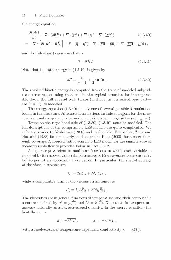
16 1. Fluid Dynamics
the energy equation
∂(ρE)∂t
+ ∇ · (ρuE) + ∇ · (pu) + ∇ · qc −∇ · (τ cu) (1.3.40)
= −∇ ·[
ρ(uE − uE)]
−∇ · (q − qc) −∇ · (pu − pu) + ∇ · (τu − τ cu) ,
and the (ideal gas) equation of state
p = ρRT . (1.3.41)
Note that the total energy in (1.3.40) is given by
ρE =p
γ − 1+
12ρu · u . (1.3.42)
The resolved kinetic energy is computed from the trace of modeled subgrid-scale stresses, assuming that, unlike the typical situation for incompress-ible flows, the full subgrid-scale tensor (and not just its anisotropic part—see (1.4.11)) is modeled.
The energy equation (1.3.40) is only one of several possible formulationsfound in the literature. Alternate formulations include equations for the pres-sure, internal energy, enthalpy, and a modified total energy ρE = ρ(e+ 1
2 u·u).Terms on the right-hand side of (1.3.39)–(1.3.40) must be modeled. The
full descriptions of the compressible LES models are quite complicated. Werefer the reader to Yoshizawa (1986) and to Speziale, Erlebacher, Zang andHussaini (1988) for some early models, and to Pope (2000) for a more thor-ough coverage. A representative complete LES model for the simpler case ofincompressible flow is provided below in Sect. 1.4.2.
A superscript c refers to nonlinear functions in which each variable isreplaced by its resolved value (simple average or Favre average as the case maybe) to permit an approximate evaluation. In particular, the spatial averageof the viscous stresses are
τij = 2μSij + λδijSkk ,
while a computable form of the viscous stress tensor is
τcij = 2μcSij + λcδij Skk .
The viscosities are in general functions of temperature, and their computableforms are defined by μc = μ(T ) and λc = λ(T ). Note that the temperatureappears naturally as a Favre-averaged quantity. In the energy equation, theheat fluxes are
q = −κ∇T , qc = −κc∇T ,
with a resolved-scale, temperature-dependent conductivity κc = κ(T ).
1.3 Compressible Fluid Dynamics Equations 17
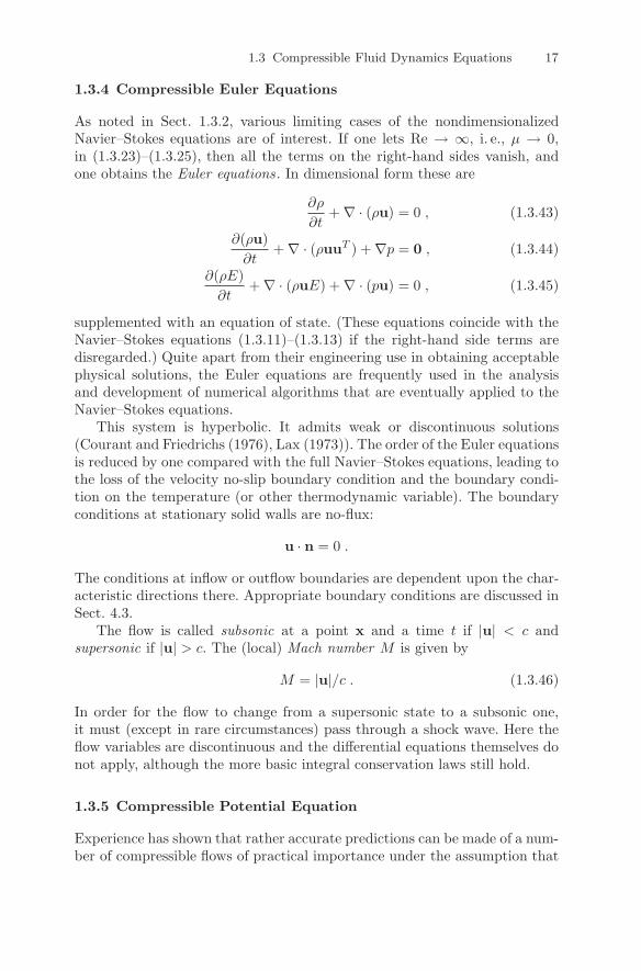
1.3.4 Compressible Euler Equations
As noted in Sect. 1.3.2, various limiting cases of the nondimensionalizedNavier–Stokes equations are of interest. If one lets Re → ∞, i. e., μ → 0,in (1.3.23)–(1.3.25), then all the terms on the right-hand sides vanish, andone obtains the Euler equations . In dimensional form these are
∂ρ
∂t+ ∇ · (ρu) = 0 , (1.3.43)
∂(ρu)∂t
+ ∇ · (ρuuT ) + ∇p = 0 , (1.3.44)
∂(ρE)∂t
+ ∇ · (ρuE) + ∇ · (pu) = 0 , (1.3.45)
supplemented with an equation of state. (These equations coincide with theNavier–Stokes equations (1.3.11)–(1.3.13) if the right-hand side terms aredisregarded.) Quite apart from their engineering use in obtaining acceptablephysical solutions, the Euler equations are frequently used in the analysisand development of numerical algorithms that are eventually applied to theNavier–Stokes equations.
This system is hyperbolic. It admits weak or discontinuous solutions(Courant and Friedrichs (1976), Lax (1973)). The order of the Euler equationsis reduced by one compared with the full Navier–Stokes equations, leading tothe loss of the velocity no-slip boundary condition and the boundary condi-tion on the temperature (or other thermodynamic variable). The boundaryconditions at stationary solid walls are no-flux:
u · n = 0 .
The conditions at inflow or outflow boundaries are dependent upon the char-acteristic directions there. Appropriate boundary conditions are discussed inSect. 4.3.
The flow is called subsonic at a point x and a time t if |u| < c andsupersonic if |u| > c. The (local) Mach number M is given by
M = |u|/c . (1.3.46)
In order for the flow to change from a supersonic state to a subsonic one,it must (except in rare circumstances) pass through a shock wave. Here theflow variables are discontinuous and the differential equations themselves donot apply, although the more basic integral conservation laws still hold.
1.3.5 Compressible Potential Equation
Experience has shown that rather accurate predictions can be made of a num-ber of compressible flows of practical importance under the assumption that
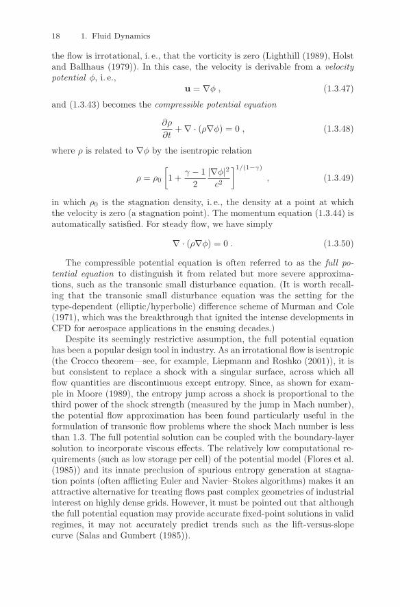
18 1. Fluid Dynamics
the flow is irrotational, i. e., that the vorticity is zero (Lighthill (1989), Holstand Ballhaus (1979)). In this case, the velocity is derivable from a velocitypotential φ, i. e.,
u = ∇φ , (1.3.47)
and (1.3.43) becomes the compressible potential equation
∂ρ
∂t+ ∇ · (ρ∇φ) = 0 , (1.3.48)
where ρ is related to ∇φ by the isentropic relation
ρ = ρ0
[
1 +γ − 1
2|∇φ|2c2
]1/(1−γ)
, (1.3.49)
in which ρ0 is the stagnation density, i. e., the density at a point at whichthe velocity is zero (a stagnation point). The momentum equation (1.3.44) isautomatically satisfied. For steady flow, we have simply
∇ · (ρ∇φ) = 0 . (1.3.50)
The compressible potential equation is often referred to as the full po-tential equation to distinguish it from related but more severe approxima-tions, such as the transonic small disturbance equation. (It is worth recall-ing that the transonic small disturbance equation was the setting for thetype-dependent (elliptic/hyperbolic) difference scheme of Murman and Cole(1971), which was the breakthrough that ignited the intense developments inCFD for aerospace applications in the ensuing decades.)
Despite its seemingly restrictive assumption, the full potential equationhas been a popular design tool in industry. As an irrotational flow is isentropic(the Crocco theorem—see, for example, Liepmann and Roshko (2001)), it isbut consistent to replace a shock with a singular surface, across which allflow quantities are discontinuous except entropy. Since, as shown for exam-ple in Moore (1989), the entropy jump across a shock is proportional to thethird power of the shock strength (measured by the jump in Mach number),the potential flow approximation has been found particularly useful in theformulation of transonic flow problems where the shock Mach number is lessthan 1.3. The full potential solution can be coupled with the boundary-layersolution to incorporate viscous effects. The relatively low computational re-quirements (such as low storage per cell) of the potential model (Flores et al.(1985)) and its innate preclusion of spurious entropy generation at stagna-tion points (often afflicting Euler and Navier–Stokes algorithms) makes it anattractive alternative for treating flows past complex geometries of industrialinterest on highly dense grids. However, it must be pointed out that althoughthe full potential equation may provide accurate fixed-point solutions in validregimes, it may not accurately predict trends such as the lift-versus-slopecurve (Salas and Gumbert (1985)).
1.3 Compressible Fluid Dynamics Equations 19
The desire for efficient numerical solutions of (1.3.50) for use in aircraft de-sign motivated considerable progress in computational fluid dynamics in thelate 1970s and early 1980s; see, e. g., Jameson (1978) and Glowinski (1984).
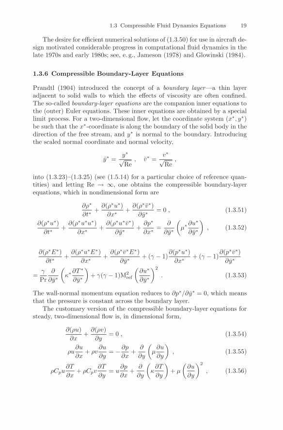
1.3.6 Compressible Boundary-Layer Equations
Prandtl (1904) introduced the concept of a boundary layer—a thin layeradjacent to solid walls to which the effects of viscosity are often confined.The so-called boundary-layer equations are the companion inner equations tothe (outer) Euler equations. These inner equations are obtained by a speciallimit process. For a two-dimensional flow, let the coordinate system (x∗, y∗)be such that the x∗-coordinate is along the boundary of the solid body in thedirection of the free stream, and y∗ is normal to the boundary. Introducingthe scaled normal coordinate and normal velocity,
y∗ =y∗√Re
, v∗ =v∗√Re
,
into (1.3.23)–(1.3.25) (see (1.5.14) for a particular choice of reference quan-tities) and letting Re → ∞, one obtains the compressible boundary-layerequations, which in nondimensional form are
∂ρ∗
∂t∗+∂(ρ∗u∗)∂x∗
+∂(ρ∗v∗)∂y∗
= 0 , (1.3.51)
∂(ρ∗u∗)∂t∗
+∂(ρ∗u∗u∗)∂x∗
+∂(ρ∗u∗v∗)∂y∗
+∂p∗
∂x∗=
∂
∂y∗
(
μ∗∂u∗
∂y∗
)
, (1.3.52)
∂(ρ∗E∗)∂t∗
+∂(ρ∗u∗E∗)∂x∗
+∂(ρ∗v∗E∗)∂y∗
+ (γ − 1)∂(p∗u∗)∂x∗
+ (γ − 1)∂(p∗v∗)∂y∗
=γ
Pr∂
∂y∗
(
κ∗∂T ∗
∂y∗
)
+ γ(γ − 1)M2ref
(∂u∗
∂y∗
)2
. (1.3.53)
The wall-normal momentum equation reduces to ∂p∗/∂y∗ = 0, which meansthat the pressure is constant across the boundary layer.
The customary version of the compressible boundary-layer equations forsteady, two-dimensional flow is, in dimensional form,
∂(ρu)∂x
+∂(ρv)∂y
= 0 , (1.3.54)
ρu∂u
∂x+ ρv
∂u
∂y= − ∂p
∂x+∂
∂y
(
μ∂u
∂y
)
, (1.3.55)
ρCpu∂T
∂x+ ρCpv
∂T
∂y= u
∂p
∂x+∂
∂y
(
κ∂T
∂y
)
+ μ(∂u
∂y
)2
, (1.3.56)
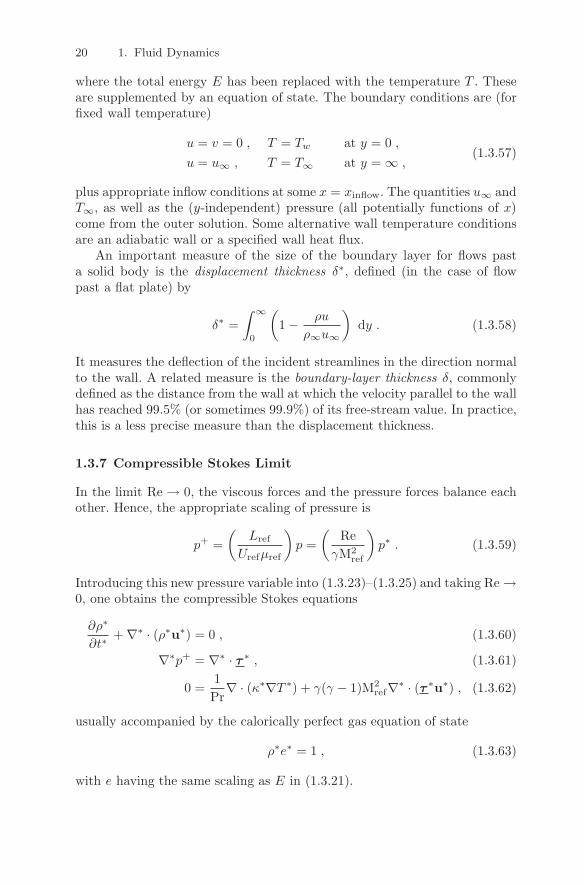
20 1. Fluid Dynamics
where the total energy E has been replaced with the temperature T . Theseare supplemented by an equation of state. The boundary conditions are (forfixed wall temperature)
u = v = 0 , T = Tw at y = 0 ,u = u∞ , T = T∞ at y = ∞ ,
(1.3.57)
plus appropriate inflow conditions at some x = xinflow. The quantities u∞ andT∞, as well as the (y-independent) pressure (all potentially functions of x)come from the outer solution. Some alternative wall temperature conditionsare an adiabatic wall or a specified wall heat flux.
An important measure of the size of the boundary layer for flows pasta solid body is the displacement thickness δ∗, defined (in the case of flowpast a flat plate) by
δ∗ =∫ ∞
0
(
1 − ρu
ρ∞u∞
)
dy . (1.3.58)
It measures the deflection of the incident streamlines in the direction normalto the wall. A related measure is the boundary-layer thickness δ, commonlydefined as the distance from the wall at which the velocity parallel to the wallhas reached 99.5% (or sometimes 99.9%) of its free-stream value. In practice,this is a less precise measure than the displacement thickness.
1.3.7 Compressible Stokes Limit
In the limit Re → 0, the viscous forces and the pressure forces balance eachother. Hence, the appropriate scaling of pressure is
p+ =(
Lref
Urefμref
)
p =(
ReγM2
ref
)
p∗ . (1.3.59)
Introducing this new pressure variable into (1.3.23)–(1.3.25) and taking Re →0, one obtains the compressible Stokes equations
∂ρ∗
∂t∗+ ∇∗ · (ρ∗u∗) = 0 , (1.3.60)
∇∗p+ = ∇∗ · τ ∗ , (1.3.61)
0 =1Pr
∇ · (κ∗∇T ∗) + γ(γ − 1)M2ref∇∗ · (τ ∗u∗) , (1.3.62)
usually accompanied by the calorically perfect gas equation of state
ρ∗e∗ = 1 , (1.3.63)
with e having the same scaling as E in (1.3.21).
1.4 Incompressible Fluid Dynamics Equations 21
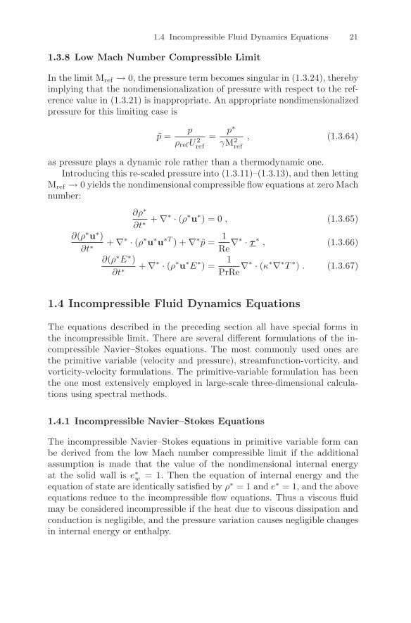
1.3.8 Low Mach Number Compressible Limit
In the limit Mref → 0, the pressure term becomes singular in (1.3.24), therebyimplying that the nondimensionalization of pressure with respect to the ref-erence value in (1.3.21) is inappropriate. An appropriate nondimensionalizedpressure for this limiting case is
p =p
ρrefU2ref
=p∗
γM2ref
, (1.3.64)
as pressure plays a dynamic role rather than a thermodynamic one.Introducing this re-scaled pressure into (1.3.11)–(1.3.13), and then letting
Mref → 0 yields the nondimensional compressible flow equations at zero Machnumber:
∂ρ∗
∂t∗+ ∇∗ · (ρ∗u∗) = 0 , (1.3.65)
∂(ρ∗u∗)∂t∗
+ ∇∗ · (ρ∗u∗u∗T ) + ∇∗p =1
Re∇∗ · τ ∗ , (1.3.66)
∂(ρ∗E∗)∂t∗
+ ∇∗ · (ρ∗u∗E∗) =1
PrRe∇∗ · (κ∗∇∗T ∗) . (1.3.67)
1.4 Incompressible Fluid Dynamics Equations
The equations described in the preceding section all have special forms inthe incompressible limit. There are several different formulations of the in-compressible Navier–Stokes equations. The most commonly used ones arethe primitive variable (velocity and pressure), streamfunction-vorticity, andvorticity-velocity formulations. The primitive-variable formulation has beenthe one most extensively employed in large-scale three-dimensional calcula-tions using spectral methods.
1.4.1 Incompressible Navier–Stokes Equations
The incompressible Navier–Stokes equations in primitive variable form canbe derived from the low Mach number compressible limit if the additionalassumption is made that the value of the nondimensional internal energyat the solid wall is e∗w = 1. Then the equation of internal energy and theequation of state are identically satisfied by ρ∗ = 1 and e∗ = 1, and the aboveequations reduce to the incompressible flow equations. Thus a viscous fluidmay be considered incompressible if the heat due to viscous dissipation andconduction is negligible, and the pressure variation causes negligible changesin internal energy or enthalpy.
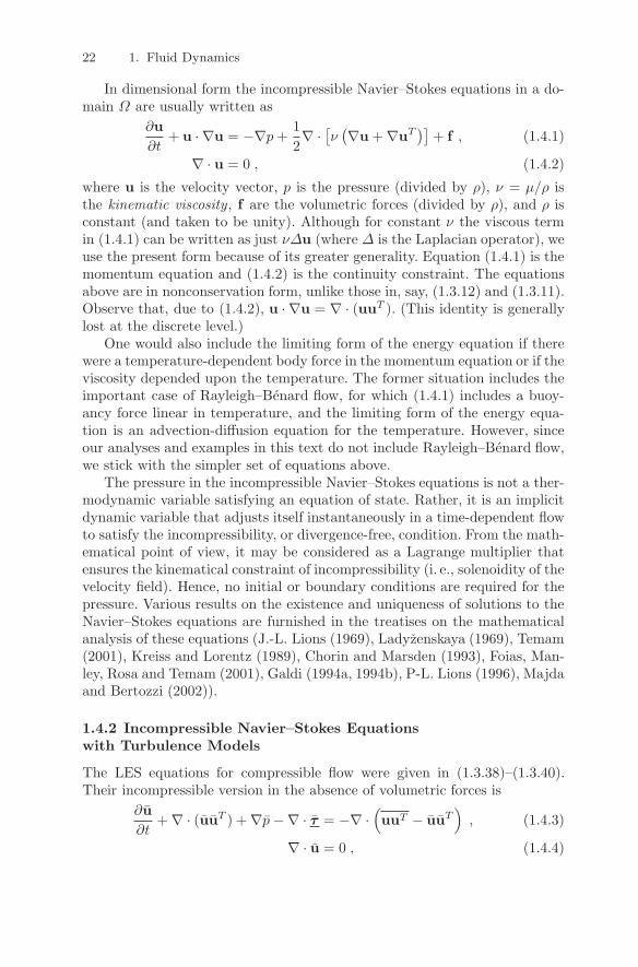
22 1. Fluid Dynamics
In dimensional form the incompressible Navier–Stokes equations in a do-main Ω are usually written as
∂u∂t
+ u · ∇u = −∇p+12∇ ·[
ν(
∇u + ∇uT)]
+ f , (1.4.1)
∇ · u = 0 , (1.4.2)
where u is the velocity vector, p is the pressure (divided by ρ), ν = μ/ρ isthe kinematic viscosity, f are the volumetric forces (divided by ρ), and ρ isconstant (and taken to be unity). Although for constant ν the viscous termin (1.4.1) can be written as just νΔu (where Δ is the Laplacian operator), weuse the present form because of its greater generality. Equation (1.4.1) is themomentum equation and (1.4.2) is the continuity constraint. The equationsabove are in nonconservation form, unlike those in, say, (1.3.12) and (1.3.11).Observe that, due to (1.4.2), u · ∇u = ∇ · (uuT ). (This identity is generallylost at the discrete level.)
One would also include the limiting form of the energy equation if therewere a temperature-dependent body force in the momentum equation or if theviscosity depended upon the temperature. The former situation includes theimportant case of Rayleigh–Benard flow, for which (1.4.1) includes a buoy-ancy force linear in temperature, and the limiting form of the energy equa-tion is an advection-diffusion equation for the temperature. However, sinceour analyses and examples in this text do not include Rayleigh–Benard flow,we stick with the simpler set of equations above.
The pressure in the incompressible Navier–Stokes equations is not a ther-modynamic variable satisfying an equation of state. Rather, it is an implicitdynamic variable that adjusts itself instantaneously in a time-dependent flowto satisfy the incompressibility, or divergence-free, condition. From the math-ematical point of view, it may be considered as a Lagrange multiplier thatensures the kinematical constraint of incompressibility (i. e., solenoidity of thevelocity field). Hence, no initial or boundary conditions are required for thepressure. Various results on the existence and uniqueness of solutions to theNavier–Stokes equations are furnished in the treatises on the mathematicalanalysis of these equations (J.-L. Lions (1969), Ladyzenskaya (1969), Temam(2001), Kreiss and Lorentz (1989), Chorin and Marsden (1993), Foias, Man-ley, Rosa and Temam (2001), Galdi (1994a, 1994b), P-L. Lions (1996), Majdaand Bertozzi (2002)).
1.4.2 Incompressible Navier–Stokes Equationswith Turbulence Models
The LES equations for compressible flow were given in (1.3.38)–(1.3.40).Their incompressible version in the absence of volumetric forces is
∂u∂t
+ ∇ · (uuT ) + ∇p−∇ · τ = −∇ ·(
uuT − uuT)
, (1.4.3)
∇ · u = 0 , (1.4.4)
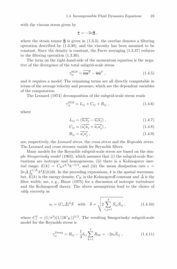
1.4 Incompressible Fluid Dynamics Equations 23
with the viscous stress given by
τ = −2νS ,
where the strain tensor S is given in (1.3.3), the overbar denotes a filteringoperation described by (1.3.30), and the viscosity has been assumed to beconstant. Since the density is constant, the Favre averaging (1.3.37) reducesto the filtering operation (1.3.30).
The term on the right-hand-side of the momentum equation is the nega-tive of the divergence of the total subgrid-scale stress
τSGSij = uuT − uuT , (1.4.5)
and it requires a model. The remaining terms are all directly computable interms of the average velocity and pressure, which are the dependent variablesof the computation.
The Leonard (1974) decomposition of the subgrid-scale stress reads
τSGSij = Lij + Cij +Rij , (1.4.6)
where
Lij = (uiuj − uiuj) , (1.4.7)
Cij = (u′iuj + uiu′j) , (1.4.8)
Rij = u′iu′j , (1.4.9)
are, respectively, the Leonard stress , the cross stress and the Reynolds stress .The Leonard and cross stresses vanish for Reynolds filters.
Many models for the Reynolds subgrid-scale stress are based on the sim-ple Smagorinsky model (1963), which assumes that (i) the subgrid-scale fluc-tuations are isotropic and homogeneous, (ii) there is a Kolmogorov iner-tial range, E(k) = CKε
2/3k−5/3, and (iii) the mean dissipation rate ε =2νΔ
∫ 1/Δ
0k2E(k)dk. In the preceding expressions, k is the spatial wavenum-
ber, E(k) is the energy density, CK is the Kolmogoroff constant and Δ is thefilter width; see, e. g., Hinze (1975) for a discussion of isotropic turbulenceand the Kolmogoroff theory. The above assumptions lead to the choice ofeddy viscosity as
νt = (CsΔ)2S with S =
√√√√2
3∑
i,j=1
Sij Sij , (1.4.10)
where C2s = (1/π2)(1/(3CK))3/2. The resulting Smagorinsky subgrid-scale
model for the Reynolds stress is
τSmagij = Rij −
13δij
3∑
k=1
Rkk = −2νtSij , (1.4.11)

24 1. Fluid Dynamics
with νt given by (1.4.10). Typically,
Δ = 2(ΔxΔyΔz)1/3 , (1.4.12)
with Δx, Δy and Δz the computational grid spacings in the three coordinatedirections. The Smagorinsky constant is usually taken to be Cs ≈ 0.1. (Wecaution the reader that several different conventions are used for this model;one will often not see a factor of 2 inside the square root in (1.4.10), andsometimes the Smagorinksy constant Cs is not squared.) Note that only theanisotropic part of the Reynolds stress is modeled. The isotropic part
13δij
3∑
k=1
Rkk
can be absorbed into the pressure for incompressible flow (but not, of course,for compressible flow).
One improvement to this model that is often employed is the dynamicSmagorinsky model , which was proposed by Germano, Piomelli, Moin andCabot (1991) and refined by Lilly (1992). This uses filters with two differentwidths to make the “constant” Cs depend upon time and usually also uponspace. In addition to the grid filter on the scale Δ, one also employs a largertest filter on the scale Δ (usually Δ = 2Δ). One then defines the so-calledresolved turbulent stresses τSGS,resolved and the subtest stresses τSGS,subtest,given by
τSGS,resolvedij = uiuj − ˆui ˆuj , τSGS,subtest
ij = uiuj − ˆui ˆuj . (1.4.13)
Then, the modeling assumption
τSGSij − 1
3δij
3∑
k=1
τSGSkk = −2Csαij ,
τSGS,subtest − 13δij
3∑
k=1
τSGS,subtestkk = −2Cdβij ,
(1.4.14)
for some tensors α and β is made. There are several choices for these tensors.One simple choice is
αij = Δ2|ˆS| ˆSij , βij = Δ2|S|Sij . (1.4.15)
Upon substitution of (1.4.14) into the Germano identity (Germano (1992)),
τSGS,resolvedij = τSGS,subtest
ij − τSGSij , (1.4.16)
1.4 Incompressible Fluid Dynamics Equations 25
and invocation of a least-squares minimization process, the dynamic Sma-gorinsky “constant” Cd is then computed from
Cd = −12<∑3
i,j=1 τSGS,resolvedij γij >
<∑3
i,j=1 γijγij >, (1.4.17)
where γij = βij − αij , and < · > represents an appropriate spatial averagingprocess. For example, in the case of homogeneous turbulence this would bea full three-dimensional spatial average, whereas for more complex flows, thespatial averaging would be more localized. All the quantities in (1.4.17) de-pend either directly upon the dependent variables in the LES computation,i. e., the βij , or can be computed by application of the test filter to the depen-dent variables, i. e., τSGS,resolved
ij and αij . (See Germano et al. (1991), Lilly(1992), Piomelli (2004), or Sagaut (2006) for more details and refinements.)
Alternative approaches to turbulence modeling based on the use of sepa-rate equations for the large and small scales, with the modeling confined toterms in the equations for the small scales, have been taken by Temam andcoworkers (see, e. g., Dubois, Jauberteau and Temam (1998)) with the so-called nonlinear Galerkin method, and by Hughes and coworkers (see, e. g.,the review paper by Hughes, Scovazzi and Franca (2004)) with the so-calledvariational multiscale method. They differ in the models used for the un-resolved terms. These models are intrinsically connected to the underlyingdiscretization and cannot be directly described solely in terms of a PDE sys-tem, as can the models already described. We defer further description toSect. 3.3.5, where discretization approaches are discussed.
We refer the reader to the review by Lesieur and Metais (1996) and thetext by Sagaut (2006) for thorough discussions of the subtle issues and thevarious subgrid-scale models that have been utilized in large-eddy simulationof incompressible flows. Some mathematical aspects of LES are discussed inBerselli, Iliescu and Layton (2006). RANS models for incompressible flow arevery well-developed. As spectral methods have rarely been applied to RANS,we simply refer to Speziale (1991), Wilcox (1993), Chen and Jaw (1998) andBernard and Wallace (2002) as some standard references on the subject.
1.4.3 Vorticity–Streamfunction Equations
One of the most interesting characteristics of a flow is its vorticity. This isdenoted by ω and is given by
ω = ∇× u . (1.4.18)
It represents (half) the local rotation rate of the fluid. A dynamical equationfor the vorticity is derived by taking the curl of (1.4.1), which for the constantviscosity, unforced case yields
∂ω
∂t+ u · ∇ω = ω · ∇u + νΔω . (1.4.19)
26 1. Fluid Dynamics
This is an advection-diffusion equation with the additional term ω ·∇u. Thisterm represents the effects of vortex stretching. It is identically zero for two-dimensional flows and is responsible for many of the interesting aspects ofthree-dimensional flows.
The vorticity can be combined with the streamfunction ψ to yield a con-cise description of two-dimensional flows. By setting u = (u, v, 0)T , a stream-function ψ is defined by the relations
u =∂ψ
∂y, v = −∂ψ
∂x; (1.4.20)
the existence of such a function is guaranteed by the solenoidal property ofu. Taking the curl of the velocity and setting ω = (0, 0, ω)T , we obtain
Δψ = −ω . (1.4.21)
Equation (1.4.19) reduces to
∂ω
∂t+∂ψ
∂y
∂ω
∂x− ∂ψ
∂x
∂ω
∂y= νΔω . (1.4.22)
The flow is parallel to curves of constant ψ—the streamlines. In the case ofsteady, rigid walls, the boundary conditions that accompany (1.4.21)–(1.4.22)are
ψ = 0 ,∂ψ
∂n= 0 , (1.4.23)
where (∂ψ/∂n) represents the partial derivative of ψ in the direction normalto the wall.
Equations (1.4.21)–(1.4.23) provide a complete description of a two-dimensional incompressible flow; the velocity is then recovered through(1.4.20). Note that the pressure is not needed. The subtlety of the stream-function-vorticity formulation is that there are no physical boundary condi-tions on the vorticity, but two boundary conditions on the streamfunction.
The elimination of the vorticity leads to the pure streamfunction formu-lation
∂
∂t(Δψ) +
∂ψ
∂y
∂
∂x(Δψ) − ∂ψ
∂x
∂
∂y(Δψ) = νΔ2ψ . (1.4.24)
The extension of these approaches to three-dimensional flows requires theintroduction of a second streamfunction or the use of a vector potential. Theappropriate equations for the former can be found in Murdock (1986) andthose for the latter in Brosa and Grossman (2002).
1.4.4 Vorticity–Velocity Equations
Another approach to eliminating the pressure from the incompressible Navier–Stokes equations is to take the curl of the momentum equation. There are
1.5 Linear Stability of Parallel Flows 27
several versions of the resulting vorticity-velocity equations (see, e. g., Trujilloand Karniadakis (1999)). An example, for constant viscosity, is given by
∂ω
∂t+ ∇× (ω × u) = −ν∇× (∇× ω) , (1.4.25)
Δu = −∇× ω , (1.4.26)∇ · u = 0 . (1.4.27)
The initial and boundary conditions on the velocity must be supplementedwith initial and boundary conditions on the vorticity. The former are usuallyderived from the curl of the initial velocity field, and the latter from theboundary values of the curl of the instantaneous velocity field.
Although the vorticity-velocity equations have six dependent variablesinstead of the four associated with the primitive variable formulations, thereare some circumstances in which they present computational advantages. Onesimple example will be given in Sect. 3.4.1.
1.4.5 Incompressible Boundary-Layer Equations
Prandtl’s boundary-layer approximation for incompressible flow yields thefollowing lowest-order terms from (1.4.1) and (1.4.2):
u∂u
∂x+ v
∂u
∂y= − ∂p
∂x+ ν
∂2u
∂y2, (1.4.28)
∂u
∂x+∂v
∂y= 0 . (1.4.29)
The boundary conditions are
u = v = 0 at y = 0 ,u = u∞ at y = ∞ ,
(1.4.30)
plus appropriate inflow conditions at some x = x∞ and the prescribed pres-sure gradient.
1.5 Linear Stability of Parallel Flows
Even though a particular time-dependent Navier–Stokes problem may admitan equilibrium solution, i. e., a solution of the steady Navier–Stokes equations,that equilibrium solution may not be physically attainable due to instabil-ity (in time or in space) of the flow to small disturbances. The question ofwhether a given equilibrium solution is stable or unstable is crucial to manyapplications.
Rayleigh (1880) initiated the development of incompressible, inviscid lin-ear stability theory. A subsequent series of papers by Rayleigh (see Mack
28 1. Fluid Dynamics
(1984)) established the theory of linear instability of inviscid flows as aneigenvalue problem governed by a second-order ordinary differential equationfor the amplitude of the disturbance, with the disturbance wavenumber andfrequency as parameters; this equation is now known as the Rayleigh equa-tion. Apart from its importance in its own right, it provided two of the fourindependent fundamental solutions of the asymptotic viscous theory devel-oped later. A key result of the inviscid linear theory is that the existence ofan inflection point in the equilibrium velocity profile of the flow, i. e., a pointat which the curvature of the profile vanishes, is a necessary condition forinstability. In other words, there can be neither unstable nor neutral wavesin a flow characterized by a velocity profile without an inflection point. Asviscosity is supposed to have a diffusive effect, this led to the disturbing con-clusion that flows with convex velocity profiles (e. g., boundary-layer flows)are stable, which conflicts with observations.
Although the formative ideas on the destabilizing influence of viscositywere propounded in Taylor (1915) and independently by Prandtl (1921),the genesis of an asymptotic viscous theory is ascribed to Tollmien (1929)and Schlichting (1933) (see Schlichting and Gersten (1999), Mack (1984)).The viscosity-induced instability waves of unidirectional flows are usuallycalled Tollmien–Schlichting waves. The asymptotic viscous theory was puton a rather rigorous mathematical basis by Lin (1945) and Wasow (1948).Despite all these mathematical developments, the asymptotic viscous theoryonly attracted serious attention in the fluid mechanics community after itsvalidation by the landmark experiments of Schubauer and Skramsdat (1947),where unstable waves just like those predicted by the theory were observed.Since the early 1960s, the asymptotic theories have been supplanted in practi-cal applications by numerical solutions of the governing differential equations.See (Drazin and Reid (2004), Schmid and Henningson (2001), and Criminale,Jackson and Joslin (2003) for a thorough coverage of fluid dynamics stability.
In applications to flows past such vehicles as aircraft and submarines,a limitation of the linear theory is that although it can predict the criticalvalue of the Reynolds number at which instability commences, it can predictneither where the laminar boundary layer will start to break down (tran-sition onset) nor where the laminar-turbulent transition will be complete.However, linear stability theory has underpinned a semi-empirical criterion,known as the eN method, for predicting the onset of transition in low distur-bance environments. This was proposed by Smith and Gamberoni (1956) andVan Ingen (1956) and is still widely used in engineering applications (Malik(1989)). This method states that transition occurs roughly when linear the-ory predicts that an initial disturbance will have grown by a factor of eN .The optimum choice of N is application-dependent, but it is usually in therange N = 9–11.
In this section we describe the mathematical formulation of the linearstability problem for parallel flows , which are flows for which the mean flow
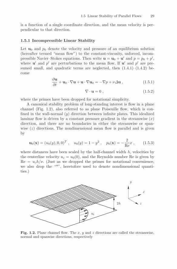
1.5 Linear Stability of Parallel Flows 29
is a function of a single coordinate direction, and the mean velocity is per-pendicular to that direction.
1.5.1 Incompressible Linear Stability
Let u0 and p0 denote the velocity and pressure of an equilibrium solution(hereafter termed “mean flow”) to the constant-viscosity, unforced, incom-pressible Navier–Stokes equations. Then write u = u0 + u′ and p = p0 + p′,where u′ and p′ are perturbations to the mean flow. If u′ and p′ are pre-sumed small, and quadratic terms are neglected, then (1.4.1)–(1.4.2) be-come
∂u∂t
+ u0 · ∇u + u · ∇u0 = −∇p+ νΔu , (1.5.1)
∇ · u = 0 , (1.5.2)
where the primes have been dropped for notational simplicity.A canonical stability problem of long-standing interest is flow in a plane
channel (Fig. 1.2), also referred to as plane Poiseuille flow, which is con-fined in the wall-normal (y) direction between infinite plates. This idealizedlaminar flow is driven by a constant pressure gradient in the streamwise (x)direction, and there are no boundaries in either the streamwise or span-wise (z) directions. The nondimensional mean flow is parallel and is givenby
u0(x) = (u0(y), 0, 0)T , u0(y) = 1 − y2 , p0(x) = − 2Rex , (1.5.3)
where distances have been scaled by the half-channel width h, velocities bythe centerline velocity uc = u0(0), and the Reynolds number Re is given byRe = uch/ν. (Just as we dropped the primes for notational convenience,we also drop the “*”, heretofore used to denote nondimensional quanti-ties.)
Fig. 1.2. Plane channel flow. The x, y and z directions are called the streamwise,normal and spanwise directions, respectively
30 1. Fluid Dynamics
The linear stability of this flow is assessed by studying perturbations ofthe form
u(x, t) = Re{
u(y)ei(αx+βz)−iωt}
,
p(x, t) = Re{
p(y)ei(αx+βz)−iωt}
,(1.5.4)
where α, β and ω are complex constants, and Re denotes the real part ofa complex quantity. (Note the slight difference between the symbols for theReynolds number (Re) and the real part (Re).) Equations (1.5.1) and (1.5.2)become, in component form,
{D2 − (α2 + β2) − iαRe u0}u− Re (Du0)v − iαRe p = −iωRe u , (1.5.5)
{D2 − (α2 + β2) − iαRe u0}v − Re Dp = −iωRe v , (1.5.6)
{D2 − (α2 + β2) − iαRe u0}w − iβRe p = −iωRe w , (1.5.7)
iαu+ Dv + iβw = 0 , (1.5.8)
where D = d/dy. The boundary conditions are
u = v = w = 0 at y = ±1 . (1.5.9)
The system (1.5.5)–(1.5.9) describes a dispersion relation between α, βand ω with Re as a parameter. If four real quantities out of α, β and ω areprescribed, then the dispersion relation constitutes an eigenvalue problemfor the remaining two real quantities. If α and β are fixed, real quantities,then ω is the complex eigenvalue. When approached in this manner, theproblem is one of temporal stability. If Im(ω) > 0, then the correspondingmode grows in time, and the mean flow will be disrupted. The equilibriumsolution, then, is unstable if a growing mode exists for any real α and β.An alternative approach to this problem is one of spatial stability. Here, ω isreal and fixed, and two relations are imposed upon α and β to complete thespecification of the problem (Nayfeh (1980), Cebeci and Stewartson (1980)).If Im(α) > 0 or Im(β) > 0, then the mode grows in space. If such growingmodes exist for any real ω and for any orientations of the waves, then theflow is spatially unstable. Gaster (1962) has given a procedure for relatingthe results of temporal and spatial stability analyses. Huerre and Monkewitz(1990) provide a valuable discussion of the physical aspects of the spatialstability problem.
By manipulating (1.5.5)–(1.5.8) we arrive at
[D2 − (α2 + β2)]2v − iαRe u0[D2 − (α2 + β2)]v + iαRe (D2u0)v
= − iωRe [D2 − (α2 + β2)]v(1.5.10)
1.5 Linear Stability of Parallel Flows 31
and
[D2 − (α2 + β2)](αw − βu) − iαRe u0(αw − βu)
= − iωRe (αw − βu) − βRe (Du0)v .(1.5.11)
The first of these is the celebrated Orr–Sommerfeld equation, and it is sub-jected to the boundary conditions
v = Dv = 0 at y = ±1 . (1.5.12)
(The condition on Dv follows from (1.5.8) and (1.5.9).) The quantity αw−βuis the normal component of the perturbation vorticity. It satisfies
αw − βu = 0 at y = ±1 . (1.5.13)
For this reason (1.5.11) is often referred to as the vertical vorticity equation(although Herbert (1983b) called it the Squire equation). Hence, there are twodistinct classes of solutions to the sixth-order system (1.5.5)–(1.5.9). The firstclass comprises the eigenmodes of (1.5.10) and (1.5.12), with (1.5.11) servingmerely to determine the vertical vorticity of this mode. The second class hasv ≡ 0 and contains the eigenmodes of (1.5.11) and (1.5.13). Squire (1933)showed that all solutions of the second class are damped modes. Until therole of the vertical vorticity modes in the weakly nonlinear stage of transitionwas recognized in the 1980s (Herbert (1983b)), attention had been focusedalmost exclusively on the Orr–Sommerfeld solutions. Note that in the tempo-ral stability problem the eigenvalue ω enters linearly, whereas in the spatialstability problem the eigenvalue α enters nonlinearly.
There are numerous other incompressible flows whose linear stability canbe assessed by similar mathematical formulations, e. g., circular Poiseuilleflow (pipe flow), Taylor–Couette flow (flow between rotating cylinders orrotating spheres), and free shear layers. Of course, the nondimensionalizationsand coordinate systems may differ. Moreover, in many cases, e. g., Taylor–Couette flow, the set (1.5.5)–(1.5.8) of three second-order equations and onefirst-order equation cannot be reduced to the Orr–Sommerfeld and vertical-vorticity equations (1.5.12)–(1.5.13).
1.5.2 Compressible Linear Stability
The stability of compressible flows has not attracted nearly the amount ofattention devoted to the stability of incompressible flows. Indeed, there hasyet to appear a single text devoted to the subject, and it goes unmentionedin all but the most recent texts on hydrodynamic stability, such as Schmidand Henningson (2001) and Criminale, Jackson and Joslin (2003). The basicconcepts and approach to the stability theory of compressible laminar bound-ary layers are similar to those of the incompressible counterpart. However,
32 1. Fluid Dynamics
there are some fundamental differences, which will be discussed here followinga brief historical overview.
Although Kuchemann (1938) must be credited with the first attempt todevelop a compressible stability theory (which neglected the viscosity and themean temperature gradient and was thus too restrictive), it was Lees and Lin(1946) who laid the foundation of an asymptotic theory analogous to thatfor the incompressible case. This asymptotic theory was further developed byDunn (1953) and Dunn and Lin (1955). Mack (1969) provided comprehensiveviscous and inviscid instability results for the flat-plate boundary layer forMach numbers up to 10.
The first major difference from the incompressible linear stability theoryis that from a mathematical point of view, the eigenvalue problem of theincompressible parallel flow is governed by a sixth-order system of ordinarydifferential equations (sometimes reducible to a fourth-order equation anda second-order equation), whereas the linear stability of compressible parallelflow is governed by an eighth-order system of ordinary differential equations.A key result is that the normal derivative of the mass-weighted streamwisevelocity gradient (ρu′)′, where the prime stands for D = d/dy, plays thesame critical role as the curvature of the streamwise velocity (proportionalto u′′) in the incompressible theory. Consequently, the compressible flat-plateboundary layer is unstable to purely inviscid disturbances in contrast to theincompressible case where the instability, called the Tollmien–Schlichting in-stability, is of viscous origin. In supersonic boundary layers, these distur-bances (known as the first modes) are most amplified when oblique. Wallcooling stabilizes these disturbances, as it tends to eliminate the generalizedinflection point (where (ρu′)′ = 0) within the boundary layer.
A second major difference between the compressible and incompressibletheories arises in those circumstances in which the mean flow is supersonicrelative to the phase velocity of the disturbance. Whenever the relative flowis supersonic over some portion of the boundary-layer profile, there are aninfinite number of wavenumbers for the single phase velocity (Mack 1969).Associated with each of these so-called neutral disturbances is a family ofunstable disturbances. The first of these modes is called Mack’s second mode,and it is the dominant mode of instability in the hypersonic regime. Thismode is destabilized by wall cooling, as that tends to increase the region ofsupersonic relative mean flow within the boundary layer.
Following Mack’s pioneering numerical work, Malik (1982, 1990) devel-oped efficient, high-order computational techniques for the solution of com-pressible stability problems, and demonstrated the use of the theory for an-alyzing supersonic and hypersonic transition experiments (Malik 1989). Thetheory has been extended to include real gas effects and the second modedisturbances were found to be relevant in boundary-layer transition over re-entry vehicles (Malik 2003).
Flow past solid boundaries, such as the flat plate illustrated in Fig. 1.3,have been the subject of many compressible linear stability studies. The cus-
1.5 Linear Stability of Parallel Flows 33
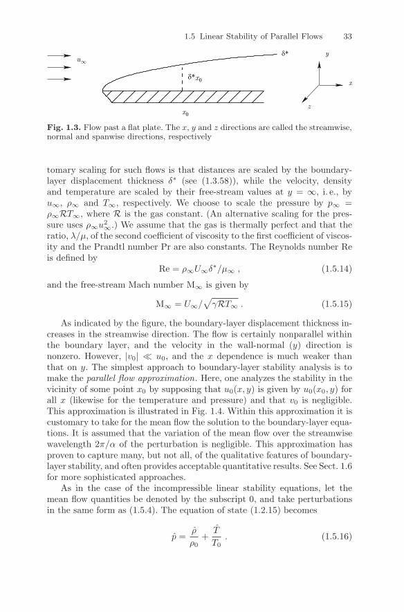
Fig. 1.3. Flow past a flat plate. The x, y and z directions are called the streamwise,normal and spanwise directions, respectively
tomary scaling for such flows is that distances are scaled by the boundary-layer displacement thickness δ∗ (see (1.3.58)), while the velocity, densityand temperature are scaled by their free-stream values at y = ∞, i. e., byu∞, ρ∞ and T∞, respectively. We choose to scale the pressure by p∞ =ρ∞RT∞, where R is the gas constant. (An alternative scaling for the pres-sure uses ρ∞u2∞.) We assume that the gas is thermally perfect and that theratio, λ/μ, of the second coefficient of viscosity to the first coefficient of viscos-ity and the Prandtl number Pr are also constants. The Reynolds number Reis defined by
Re = ρ∞U∞δ∗/μ∞ , (1.5.14)
and the free-stream Mach number M∞ is given by
M∞ = U∞/√
γRT∞ . (1.5.15)
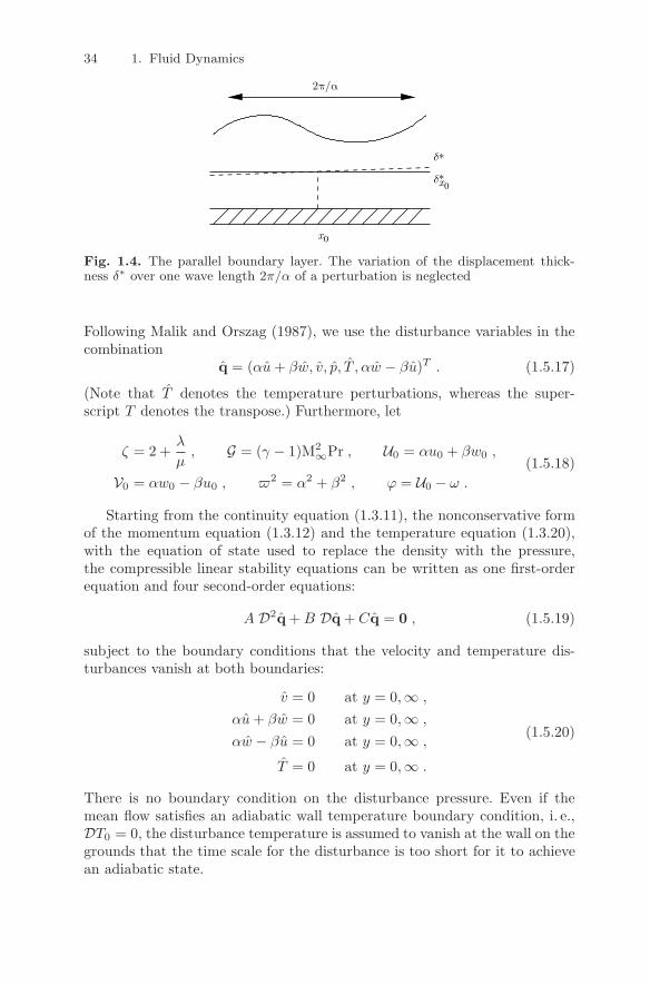
As indicated by the figure, the boundary-layer displacement thickness in-creases in the streamwise direction. The flow is certainly nonparallel withinthe boundary layer, and the velocity in the wall-normal (y) direction isnonzero. However, |v0| u0, and the x dependence is much weaker thanthat on y. The simplest approach to boundary-layer stability analysis is tomake the parallel flow approximation. Here, one analyzes the stability in thevicinity of some point x0 by supposing that u0(x, y) is given by u0(x0, y) forall x (likewise for the temperature and pressure) and that v0 is negligible.This approximation is illustrated in Fig. 1.4. Within this approximation it iscustomary to take for the mean flow the solution to the boundary-layer equa-tions. It is assumed that the variation of the mean flow over the streamwisewavelength 2π/α of the perturbation is negligible. This approximation hasproven to capture many, but not all, of the qualitative features of boundary-layer stability, and often provides acceptable quantitative results. See Sect. 1.6for more sophisticated approaches.
As in the case of the incompressible linear stability equations, let themean flow quantities be denoted by the subscript 0, and take perturbationsin the same form as (1.5.4). The equation of state (1.2.15) becomes
p =ρ
ρ0+T
T0. (1.5.16)
34 1. Fluid Dynamics
Fig. 1.4. The parallel boundary layer. The variation of the displacement thick-ness δ∗ over one wave length 2π/α of a perturbation is neglected
Following Malik and Orszag (1987), we use the disturbance variables in thecombination
q = (αu+ βw, v, p, T , αw − βu)T . (1.5.17)
(Note that T denotes the temperature perturbations, whereas the super-script T denotes the transpose.) Furthermore, let
ζ = 2 +λ
μ, G = (γ − 1)M2
∞Pr , U0 = αu0 + βw0 ,
V0 = αw0 − βu0 , �2 = α2 + β2 , ϕ = U0 − ω .(1.5.18)
Starting from the continuity equation (1.3.11), the nonconservative formof the momentum equation (1.3.12) and the temperature equation (1.3.20),with the equation of state used to replace the density with the pressure,the compressible linear stability equations can be written as one first-orderequation and four second-order equations:
A D2q +B Dq + Cq = 0 , (1.5.19)
subject to the boundary conditions that the velocity and temperature dis-turbances vanish at both boundaries:
v = 0 at y = 0,∞ ,
αu+ βw = 0 at y = 0,∞ ,
αw − βu = 0 at y = 0,∞ ,
T = 0 at y = 0,∞ .
(1.5.20)
There is no boundary condition on the disturbance pressure. Even if themean flow satisfies an adiabatic wall temperature boundary condition, i. e.,DT0 = 0, the disturbance temperature is assumed to vanish at the wall on thegrounds that the time scale for the disturbance is too short for it to achievean adiabatic state.
1.5 Linear Stability of Parallel Flows 35
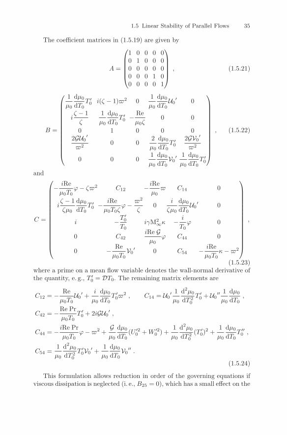
The coefficient matrices in (1.5.19) are given by
A =
⎛
⎜⎜⎜⎜⎝
1 0 0 0 00 1 0 0 00 0 0 0 00 0 0 1 00 0 0 0 1
⎞
⎟⎟⎟⎟⎠
, (1.5.21)
B =
⎛
⎜⎜⎜⎜⎜⎜⎜⎜⎜⎜⎜⎜⎝
1μ0
dμ0
dT0T ′
0 i(ζ − 1)�2 01μ0
dμ0
dT0U0
′ 0
iζ − 1ζ
1μ0
dμ0
dT0T ′
0 − Reμ0ζ
0 0
0 1 0 0 02GU0
′
�20 0
2μ0
dμ0
dT0T ′
0
2GV0′
�2
0 0 01μ0
dμ0
dT0V0
′ 1μ0
dμ0
dT0T ′
0
⎞
⎟⎟⎟⎟⎟⎟⎟⎟⎟⎟⎟⎟⎠
, (1.5.22)
and
C =
⎛
⎜⎜⎜⎜⎜⎜⎜⎜⎜⎜⎜⎜⎜⎜⎝
− iReμ0T0
ϕ− ζ�2 C12 − iReμ0� C14 0
iζ − 1ζμ0
dμ0
dT0T ′
0 − iReμ0T0ζ
ϕ− �2
ζ0
i
ζμ0
dμ0
dT0U0
′ 0
i −T′0
T0iγM2∞κ − i
T0ϕ 0
0 C42iRe Gμ0
ϕ C44 0
0 − Reμ0T0
V0′ 0 C54 − iRe
μ0T0κ−�2
⎞
⎟⎟⎟⎟⎟⎟⎟⎟⎟⎟⎟⎟⎟⎟⎠
,
(1.5.23)where a prime on a mean flow variable denotes the wall-normal derivative ofthe quantity, e. g., T ′
0 = DT0. The remaining matrix elements are
C12 = − Reμ0T0
U0′ +
i
μ0
dμ0
dT0T ′
0�2 , C14 = U0
′ 1μ0
d2μ0
dT 20
T ′0 + U0
′′ 1μ0
dμ0
dT0,
C42 = −Re Prμ0T0
T ′0 + 2iGU0
′ ,
C44 = − iRe Prμ0T0
ϕ−�2 +Gμ0
dμ0
dT0(U ′2
0 +W ′20 ) +
1μ0
d2μ0
dT 20
(T ′0)
2 +1μ0
dμ0
dT0T ′′
0 ,
C54 =1μ0
d2μ0
dT 20
T ′0V0
′ +1μ0
dμ0
dT0V0
′′ .
(1.5.24)
This formulation allows reduction in order of the governing equations ifviscous dissipation is neglected (i. e., B25 = 0), which has a small effect on the
36 1. Fluid Dynamics
unstable eigenvalue for small Mach numbers. Other forms of the compressiblestability equations are given in Malik (1990).
1.6 Stability Equations for Nonparallel Flows
Only since the late 1970s have more sophisticated approaches than theparallel-flow assumption been employed for the study of the stability ofnonparallel flows. These approaches include matched asymptotic expansions,triple-deck theory and parabolized equations. We shall focus here on the lat-ter, as spectral methods have rarely been used in the context of the otherapproaches.
The parabolized stability equations (PSE) approach was developed forincompressible flow by Herbert (1991). Further details and developmentscan be found in Bertolotti (1991) and Bertolotti et al. (1992) for incom-pressible flows, and in Chang et al. (1991), Bertolotti and Herbert (1991)for compressible flow and Malik (2003) for hypersonic flow including chem-istry effects. Schmid and Henningson (2001) furnish detailed derivationsand equations for the incompressible case. Herbert (1997) reviews applica-tions of PSE to both linear and nonlinear stability problems, for incom-pressible as well as compressible flows. The PSE permit the stability ana-lysis of many mean flows that depend upon both the streamwise and wall-normal directions. These include flow past a flat plate (see Fig. 1.3), as wellas flows of engineering interest such as flow past an airplane or a subma-rine.
The parabolized stability equations are developed by representing the to-tal flow as a mean flow plus a disturbance field and decomposing the distur-bance into a rapidly varying wave-like part and a slowly varying shape func-tion. As a complete description of the PSE would take up several pages, weconfine ourselves here to just providing an outline of the approach and illus-trating the mathematical structure of the equations, using two-dimensionalincompressible flow as the setting. Let q = (u, v, p)T represent the distur-bance field and write
q(x, y, t) = Re {q(x, y)χ(x, t)} , (1.6.1)
with
χ(x, t) = exp(
i
∫ x
x0
α(ψ) dψ − ωt)
, (1.6.2)
where α(x) is a local complex wavenumber that captures the rapidly varyingpart, ω is the frequency, and q is the slowly varying (in x) shape function.Constraints of the type
∫ ∞
0
(
¯u∂u
∂x+ ¯v
∂v
∂x
)
dy = 0 , (1.6.3)
1.6 Stability Equations for Nonparallel Flows 37
where the overbar denotes the complex conjugate, impose a condition on α(x)such that most of the waviness and growth of the disturbance are absorbedinto the exponential function χ in (1.6.2), making the shape function q slowlyvarying with x. The ellipticity is retained for the wave part while paraboliza-tion is applied to the shape function. Hence, the qxx terms in the governingequations are dropped, and we arrive at a set of equations in which the onlysecond-order derivatives are those with respect to y.
The linear parabolized stability equations are derived from the Navier–Stokes equations with the usual linearization procedure plus the paraboliza-tion approach discussed above. The linear PSE may be written as
∂q∂x
= L0q + L1∂q∂y
+ L2∂2q∂y2
. (1.6.4)
The boundary conditions are
u = 0 , v = 0 at y = 0,∞ , (1.6.5)
supplemented with appropriate inflow conditions at x = x0.The matrices in (1.6.4) are given by
L0 =
⎛
⎜⎜⎜⎜⎝
−iα 0 0
0 −iα+iω
u0− α2
u0Re− 1u0
∂v0∂y
0
iω − α2
Re− ∂u0
∂x−∂u0
∂y−iα
⎞
⎟⎟⎟⎟⎠
,
L1 =
⎛
⎜⎝
0 −1 0
0 − v0u0
− 1u0
−v0 u0 0
⎞
⎟⎠ , L2 =
⎛
⎜⎜⎜⎝
0 0 0
01
Re u00
1Re
0 0
⎞
⎟⎟⎟⎠.
(1.6.6)
Note that α is a complex function of x, u0 and v0 are real functions of xand y, and Re and ω are real constants.
For the nonlinear PSE approximation, the disturbance function can beexpressed by the following truncated Fourier series
q(x, y, t) =M∑
m=−M
qm(x, y)χm(x, t) + complex conjugate , (1.6.7)
where
χm(x, t) = exp(
i
∫ x
x0
αm(ψ)dψ −mωt)
. (1.6.8)
Following a similar parabolization strategy, one obtains for each Fourier modeqm(x, y) an equation that is structurally the same as (1.6.4) with the additionof a forcing term that accounts for the nonlinear interactions.
38 1. Fluid Dynamics
For further details, see Bertolotti, Herbert and Spalart (1992) for the full,nonlinear PSE description of incompressible flow, and see Chang et al. (1991)and Bertolotti and Herbert (1991) for the compressible formulation.
Finally, we conclude this survey with some brief remarks on triple decktheory. One line of approach has employed triple deck theory, (e. g., Smith(1979) and Hall (1983)), to derive a set of equations based on formal asymp-totic expansions to account consistently for the spatial evolution of the meanflow and the instability. As the triple deck approaches have invariably em-ployed finite-difference methods, we shall not discuss them further. (Thereappears to be no fundamental obstacle to the use of spectral methods for thetriple deck approach.)
http://www.springer.com/978-3-540-30727-3