1

Foundations of Probabilistic Answers to Queries

Dan Suciu and Nilesh Dalvi

University of Washington

2

Databases Today are Deterministic

• An item either is in the database or is not

• A tuple either is in the query answer or is not

• This applies to all variety of data models:– Relational, E/R, NF2, hierarchical, XML, …

3

What is a Probabilistic Database ?

• “An item belongs to the database” is a probabilistic event

• “A tuple is an answer to the query” is a probabilistic event

• Can be extended to all data models; we discuss only probabilistic relational data

4

Two Types of Probabilistic Data

• Database is deterministicQuery answers are probabilistic

• Database is probabilisticQuery answers are probabilistic

5

Long History

Probabilistic relational databases have been studied from the late 80’s until today:

• Cavallo&Pitarelli:1987• Barbara,Garcia-Molina, Porter:1992• Lakshmanan,Leone,Ross&Subrahmanian:1997• Fuhr&Roellke:1997• Dalvi&S:2004• Widom:2005

6

So, Why Now ?

Application pull:

• The need to manage imprecisions in data

Technology push:

• Advances in query processing techniques

The tutorial is built on these two themesThe tutorial is built on these two themes

7

Application Pull

Need to manage imprecisions in data• Many types: non-matching data values, imprecise

queries, inconsistent data, misaligned schemas, etc, etc

The quest to manage imprecisions = major driving force in the database community

• Ultimate cause for many research areas: data mining, semistructured data, schema matching, nearest neighbor

8

Theme 1:Theme 1:

A large class of imprecisions in datacan be modeled with probabilities

9

Technology Push

Processing probabilistic data is fundamentally more complex than other data models

• Some previous approaches sidestepped complexity

There exists a rich collection of powerful, non-trivial techniques and results, some old, some very recent, that could lead to practical management techniques for probabilistic databases.

10

Theme 2:Theme 2:

Identify the source of complexity,present snapshots of non-trivial results,set an agenda for future research.

11

Some Notes on the Tutorial

There is a huge amount of related work:

probabilistic db, top-k answers, KR, probabilistic reasoning, random graphs, etc, etc.

We left out many references

All references used are available in separate document

Tutorial available at: http://www.cs.washington.edu/homes/suciu

Requires TexPoint to view http://www.thp.uni-koeln.de/~ang/texpoint/index.html

12

Overview

Part I: Applications: Managing Imprecisions

Part II: A Probabilistic Data Semantics

Part III: Representation Formalisms

Part IV: Theoretical foundations

Part V: Algorithms, Implementation Techniques

Summary, Challenges, Conclusions

BREAK

13

Part I

Applications: Managing Imprecisions

14

Outline

1. Ranking query answers

2. Record linkage

3. Quality in data integration

4. Inconsistent data

5. Information disclosure

15

1. Ranking Query Answers

Database is deterministic

The query returns a ranked list of tuples

• User interested in top-k answers.

16

The Empty Answers ProblemQuery is overspecified: no answersExample: try to buy a house in

Seattle…SELECT *FROM HousesWHERE bedrooms = 4 AND style = ‘craftsman’ AND district = ‘View Ridge’ AND price < 400000

SELECT *FROM HousesWHERE bedrooms = 4 AND style = ‘craftsman’ AND district = ‘View Ridge’ AND price < 400000

[Agrawal,Chaudhuri,Das,Gionis 2003]

… good luck !Today users give up and move to Baltimore

17

Ranking:Compute a similarity score between a tuple and the query

Q = SELECT * FROM R WHERE A1=v1 AND … AND Am=vm

Q = SELECT * FROM R WHERE A1=v1 AND … AND Am=vm

[Agrawal,Chaudhuri,Das,Gionis 2003]

Rank tuples by their TF/IDF similarity to the query Q

Q = (v1, …, vm)Q = (v1, …, vm)

T = (u1, …, um)T = (u1, …, um)

Query is a vector:

Tuple is a vector:

Includes partial matches

18

Similarity Predicates in SQLBeyond a single table: “Find the good deals in a neighborhood !”

[Motro:1988,Dalvi&S:2004]

SELECT *FROM Houses xWHERE x.bedrooms ~ 4 AND x.style ~ ‘craftsman’ AND x.price ~ 600k AND NOT EXISTS (SELECT * FROM Houses y WHERE x.district = y.district AND x.ID != y.ID AND y.bedrooms ~ 4 AND y.style ~ ‘craftsman’ AND y.price ~ 600k

SELECT *FROM Houses xWHERE x.bedrooms ~ 4 AND x.style ~ ‘craftsman’ AND x.price ~ 600k AND NOT EXISTS (SELECT * FROM Houses y WHERE x.district = y.district AND x.ID != y.ID AND y.bedrooms ~ 4 AND y.style ~ ‘craftsman’ AND y.price ~ 600k

Users specify similarity predicates with ~System combines atomic similarities using probabilities

19

Types of Similarity Predicates

• String edit distances:– Levenstein distance, Q-gram distances

• TF/IDF scores

• Ontology distance / semantic similarity:– Wordnet

• Phonetic similarity:– SOUNDEX

[Theobald&Weikum:2002,Hung,Deng&Subrahmanian:2004]

20

Keyword Searches in Databases

Goal: • Users want to search via keywords• Do not know the schema

Techniques:• Matching objects may be scattered across physical

tables due to normalization; need on the fly joins• Score of a tuple = number of joins, plus “prestige”

based on indegree

[Hristidis&Papakonstantinou’2002,Bhalotia et al.2002]

21

Q = ‘Abiteboul’ and ‘Widom’Q = ‘Abiteboul’ and ‘Widom’

Paper Conference

Person

Author

Join sequences(tuple trees):

[Hristidis,Papakonstantinou’2002]

In

Editor

Paper

Person

Author

Person

Author

Widom

Abiteboul

Paper

Person

Author

Person

Author

Paper Conference

Widom

Abiteboul

Person

Person

Author

Paper Conference

Abiteboul

Widom

22

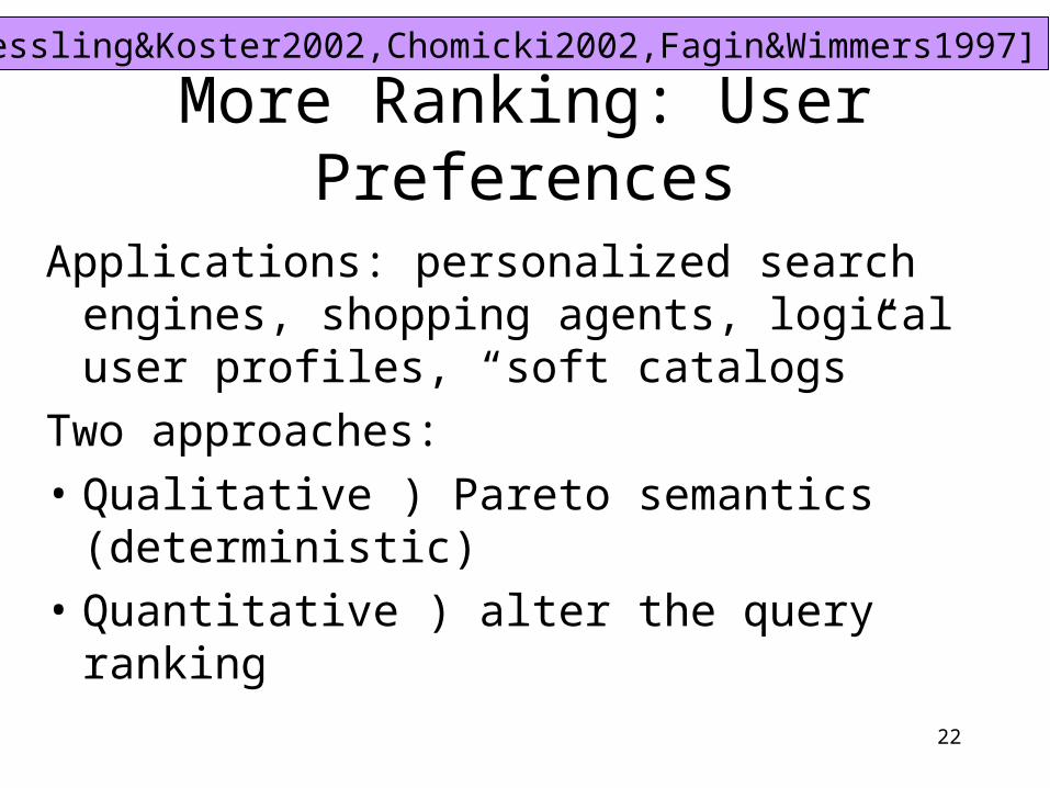
More Ranking: User Preferences

Applications: personalized search engines, shopping agents, logical user profiles, “soft catalogs”

Two approaches:

• Qualitative ) Pareto semantics (deterministic)

• Quantitative ) alter the query ranking

[Kiessling&Koster2002,Chomicki2002,Fagin&Wimmers1997]

23

Summary on Ranking Query Answers

Types of imprecision addressed:Data is precise, query answers are imprecise:• User has limited understanding of the data• User has limited understanding of the schema• User has personal preferences

Probabilistic approach would…• Principled semantics for complex queries• Integrate well with other types of imprecision

24

2. Record Linkage

Determine if two data records describe same object

Scenarios:

• Join/merge two relations• Remove duplicates from a single relation• Validate incoming tuples against a reference

[Cohen: Tutorial]

25

Fellegi-Sunter Model

A probabilistic model/framework

• Given two sets of records A, B:

Goal: partition A B into:

• Match

• Uncertain

• Non-match

[Cohen: Tutorial; Fellegi&Sunder:1969]

{a1, a2, a3, a4, a5, a6}{a1, a2, a3, a4, a5, a6}

{b1, b2, b3, b4, b5}{b1, b2, b3, b4, b5}

A =

B =

26

Non-Fellegi Sunter Approaches

Deterministic linkage• Normalize records, then test equality

– E.g. for addresses– Very fast when it works

• Hand-coded rules for an “acceptable match”– E.g. “same SSN”;or “same last name AND

same DOB”– Difficult to tune

[Cohen: Tutorial]

27

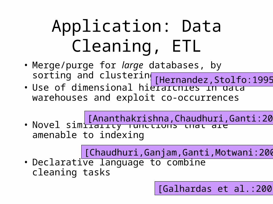
Application: Data Cleaning, ETL

• Merge/purge for large databases, by sorting and clustering

• Use of dimensional hierarchies in data warehouses and exploit co-occurrences

• Novel similarity functions that are amenable to indexing

• Declarative language to combine cleaning tasks

[Hernandez,Stolfo:1995]

[Ananthakrishna,Chaudhuri,Ganti:2002]

[Chaudhuri,Ganjam,Ganti,Motwani:2002]

[Galhardas et al.:2001]

28

Application: Data Integration

WHIRL

• All attributes in in all tables are of type text

• Datalog queries with two kinds of predicates:– Relational predicates– Similarity predicates X ~ Y

[Cohen:1998]

Matches two sets on the fly, butnot really a “record linkage” application.

Matches two sets on the fly, butnot really a “record linkage” application.

29

WHIRL

Q1(*) :- P(Company1,Industry1), Q(Company2,Website), R(Industry2, Analysis),

Company1 ~ Company2, Industry1 ~ Industry2

Q1(*) :- P(Company1,Industry1), Q(Company2,Website), R(Industry2, Analysis),

Company1 ~ Company2, Industry1 ~ Industry2

[Cohen:1998]

Score of an answer tuple = product of similarities

Example 1: datalog

30

WHIRL

[Cohen:1998]

Q2(Website) :- P(Company1,Industry1), Q(Company2,Website), R(Industry2, Analysis),

Company1 ~ Company2, Industry1 ~ Industry2

Q2(Website) :- P(Company1,Industry1), Q(Company2,Website), R(Industry2, Analysis),

Company1 ~ Company2, Industry1 ~ Industry2

score(t) = 1 - s 2 Support(t) (1-score(s))score(t) = 1 - s 2 Support(t) (1-score(s))

Support(t) = set of tuples supporting the answer t

Example 2 (with projection):

Dependson queryplan !!

31

Summary on Record LinkageTypes of imprecision addressed:Same entity represented in different ways• Misspellings, lack of canonical representation, etc.

A probability model would…• Allow system to use the match probabilities:

cheaper, on-the-fly• But need to model complex probabilistic

correlations: is one set a reference set ? how many duplicates are expected ?

32

3. Quality in Data Integration

Use of probabilistic information to reason about soundness, completeness, and overlap of sources

Applications:

• Order access to information sources

• Compute confidence scores for the answers

[Florescu,Koller,Levy97;Chang,GarciaMolina00;Mendelzon,Mihaila01]

33

Global Historical Climatology Network• Integrates climatic data from:

– 6000 temperature stations

– 7500 precipitation stations

– 2000 pressure stations

• Starting with 1697 (!!)

[Mendelzon&Mihaila:2001

Soundness of a data source: what fraction of items are correct

Completeness data source: what fractions of items it actually contains

Soundness of a data source: what fraction of items are correct

Completeness data source: what fractions of items it actually contains

34

Local as view:

[Mendelzon&Mihaila:2001

S2:S2:

S1:S1: V1(s, lat, lon, c) Station(s, lat, lon c)

V2(s, y, m, v) Temperature(s, y, m, v), Station(s, lat, lon, “Canada”), y 1900

S3:S3: V3(s, y, m, v) Temperature(s, y, m, v), Station(s, lat, lon, “US”), y 1800

S8756:S8756: . . .

. . .

Global schema: TemperatureStation

35

Next, declare soundness and complete

[Florescu,Koller,Levy:1997;Mendelzon&Mihaila:2001]

Soundness(V2) 0.7Completneess(V2) 0.4

Soundness(V2) 0.7Completneess(V2) 0.4

Precision

S2:S2: V2(s, y, m, v) Temperature(s, y, m, v), Station(s, lat, lon, “Canada”), y 1900

Recall

36

Year Value Confidence

1952 55o F 0.7

1954 -22o F 0.9

. . . . . . . . .

Goal 2: soundness ! query confidence

Q(y, v) :- Temperature(s, y, m, v), Station(s, lat, lon, “US”), y 1950, y · 1955, lat ¸ 48, lat · 49

Q(y, v) :- Temperature(s, y, m, v), Station(s, lat, lon, “US”), y 1950, y · 1955, lat ¸ 48, lat · 49

Answer:

[Mendelzon&Mihaila:2001]

Goal 1: completeness ! order source accesses

S5S5 S74

S74 S2S2 S31

S31 . . .

[Florescu,Koller,Levy:1997

37

Summary: Quality in Data Integration

Types of imprecision addressedOverlapping, inconsistent, incomplete data sources• Data is probabilistic• Query answers are probabilistic

They use already a probabilistic model• Needed: complex probabilistic spaces. E.g. a tuple

t in V1 has 60% probability of also being in V2

• Query processing still in infancy

38

4. Inconsistent Data

Goal: consistent query answers from inconsistent databases

Applications:• Integration of autonomous data sources• Un-enforced integrity constraints• Temporary inconsistencies

[Bertosi&Chomicki:2003]

39

The Repair Semantics

[Bertosi&Chomicki:2003]

Name Affiliation State Area

Miklau UW WA Data security

Dalvi UW WA Prob. Data

Balazinska UW WA Data streams

Balazinska MIT MA Data streams

Miklau Umass MA Data security

Key(?!?)

Find people in State=WA Dalvi

Hi precision, but low recallHi precision, but low recall

Find people in State=MA ;

Considerall “repairs”

40

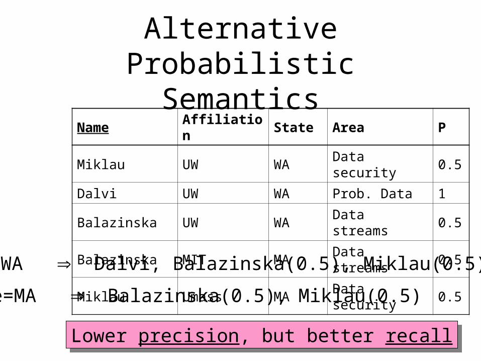
Alternative Probabilistic Semantics

Name Affiliation State Area P

Miklau UW WA Data security 0.5

Dalvi UW WA Prob. Data 1

Balazinska UW WA Data streams 0.5

Balazinska MIT MA Data streams 0.5

Miklau Umass MA Data security 0.5

State=WA Dalvi, Balazinska(0.5), Miklau(0.5)

Lower precision, but better recallLower precision, but better recall

State=MA Balazinska(0.5), Miklau(0.5)

41

Summary:Inconsistent Data

Types of imprecision addressed:• Data from different sources is contradictory• Data is uncertain, hence, arguably, probabilistic• Query answers are probabilistic

A probabilistic would…• Give better recall !• Needs to support disjoint tuple events

42

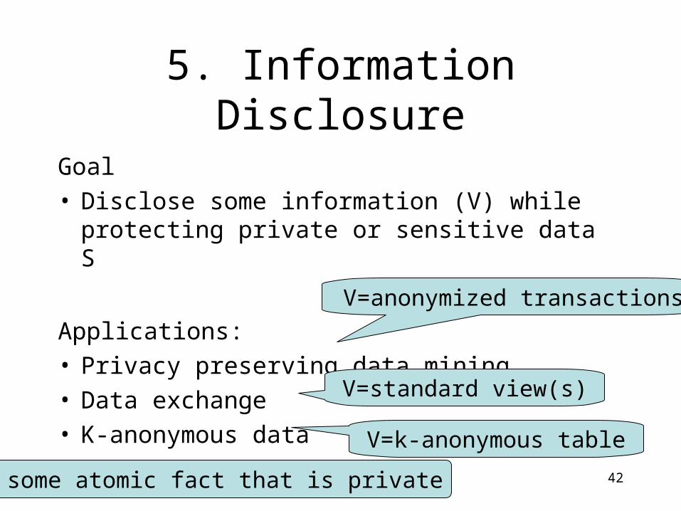
5. Information Disclosure

Goal• Disclose some information (V) while protecting

private or sensitive data S

Applications:• Privacy preserving data mining• Data exchange• K-anonymous data

V=anonymized transactions

V=standard view(s)

V=k-anonymous table

S = some atomic fact that is private

43

[Evfimievski,Gehrke,Srikant:03; Miklau&S:04;Miklau,Dalvi&S:05]

Pr(S | V)Pr(S | V)

Pr(S)Pr(S) = a priori probability of S

= a posteriori probability of S

44

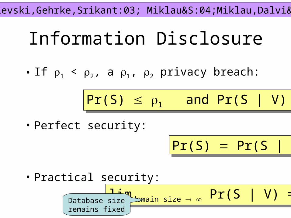
Information Disclosure

• If 1 < 2, a 1, 2 privacy breach:

• Perfect security:

• Practical security:

Pr(S) Pr(S | V)Pr(S) Pr(S | V)

limdomain size Pr(S | V) = 0limdomain size Pr(S | V) = 0

Pr(S) 1 and Pr(S | V) 2Pr(S) 1 and Pr(S | V) 2

[Evfimievski,Gehrke,Srikant:03; Miklau&S:04;Miklau,Dalvi&S:05]

Database sizeremains fixed

45

Summary:Information Disclosure

Is this a type of imprecision in data ?• Yes: it’s the adversary’s uncertainty about the

private data. • The only type of imprecision that is good

Techniques• Probabilistic methods: long history [Shannon’49]• Definitely need conditional probabilities

46

Summary:Information Disclosure

Important fundamental duality:• Query answering: want Probability . 1• Information disclosure: want Probability & 0

They share the same fundamental concepts and techniquesThey share the same fundamental concepts and techniques

47

Summary:Information Disclosure

What is required from the probabilistic model

• Don’t know the possible instances

• Express the adversary’s knowledge: – Cardinalities:– Correlations between values:

• Compute conditional probabilities

Size(Employee) ' 1000Size(Employee) ' 1000

area-code à cityarea-code à city

48

6. Other Applications

• Data lineage + accuracy: Trio

• Sensor data

• Personal information management

• Using statistics to answer queries

Semex [Dong&Halevy:2005, Dong,Halevy,Madhavan:2005]Heystack [Karger et al. 2003], Magnet [Sinha&Karger:2005]

[Deshpande, Guestrin,Madden:2004]

[Widom:2005]

[Dalvi&S;2005]

49

Summary on Part I: Applications

Common in these applications:• Data in database and/or in query answer is

uncertain, ranked; sometimes probabilisticNeed for common probabilistic model:• Main benefit: uniform approach to imprecision• Other benefits:

– Handle complex queries (instead of single table TF/IDF)– Cheaper solutions (on-the-fly record linkage)– Better recall (constraint violations)

50

Part II

A Probabilistic Data Semantics

51

Outline

• The possible worlds model

• Query semantics

52

Possible Worlds Semantics

int, char(30), varchar(55), datetimeint, char(30), varchar(55), datetime

Employee(name:varchar(55), dob:datetime, salary:int)Employee(name:varchar(55), dob:datetime, salary:int)

Attribute domains:

Relational schema:

# values: 232, 2120, 2440, 264

# of tuples: 2440 £ 264 £ 223

# of instances: 22440 £ 264 £ 223

Employee(. . .), Projects( . . . ), Groups( . . .), WorksFor( . . .)Employee(. . .), Projects( . . . ), Groups( . . .), WorksFor( . . .)

Database schema:

# of instances: N (= BIG but finite)

53

The Definition

The set of all possible database instances:

INST = {I1, I2, I3, . . ., IN}INST = {I1, I2, I3, . . ., IN}

Definition A probabilistic database Ip is a probability distribution on INST

s.t. i=1,N Pr(Ii) = 1Pr : INST ! [0,1]Pr : INST ! [0,1]

Definition A possible world is I s.t. Pr(I) > 0

will use Pr or Ip interchangeably

54

ExampleCustomer Address Product

John Seattle Gizmo

John Seattle Camera

Sue Denver Gizmo

Pr(I1) = 1/3

Customer Address Product

John Boston Gadget

Sue Denver Gizmo

Customer Address Product

John Seattle Gizmo

John Seattle Camera

Sue Seattle Camera

Customer Address Product

John Boston Gadget

Sue Seattle Camera

Pr(I2) = 1/12

Pr(I3) = 1/2Pr(I4) = 1/12

Possible worlds = {I1, I2, I3, I4}

Ip =

55

Tuples as Events

One tuple t ) event t 2 I

Two tuples t1, t2 ) event t1 2 I Æ t2 2 I

Pr(t) = I: t 2 I Pr(I)Pr(t) = I: t 2 I Pr(I)

Pr(t1 t2) = I: t1 2 I Æ t2 2 I Pr(I)Pr(t1 t2) = I: t1 2 I Æ t2 2 I Pr(I)

56

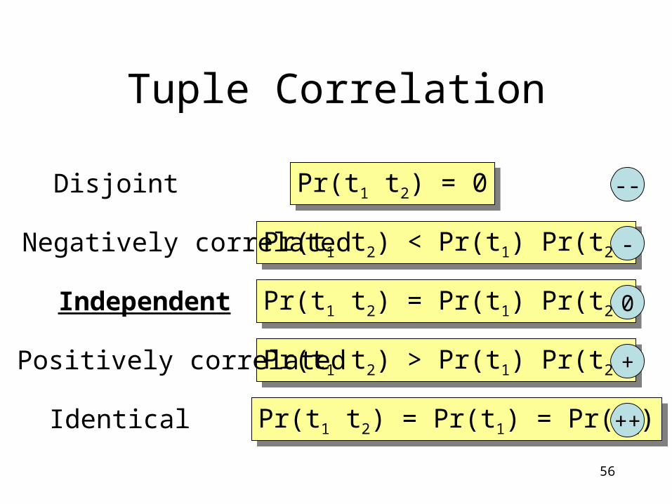
Tuple Correlation

Pr(t1 t2) = 0Pr(t1 t2) = 0Disjoint

Pr(t1 t2) < Pr(t1) Pr(t2)Pr(t1 t2) < Pr(t1) Pr(t2)Negatively correlated

Pr(t1 t2) = Pr(t1) Pr(t2)Pr(t1 t2) = Pr(t1) Pr(t2)Independent

Pr(t1 t2) > Pr(t1) Pr(t2)Pr(t1 t2) > Pr(t1) Pr(t2)Positively correlated

Pr(t1 t2) = Pr(t1) = Pr(t2)Pr(t1 t2) = Pr(t1) = Pr(t2)Identical ++

-

+

--

0

57

ExampleCustomer Address Product

John Seattle Gizmo

John Seattle Camera

Sue Denver Gizmo

Pr(I1) = 1/3

Customer Address Product

John Boston Gadget

Sue Denver Gizmo

Customer Address Product

John Seattle Gizmo

John Seattle Camera

Sue Seattle Camera

Customer Address Product

John Boston Gadget

Sue Seattle Camera

Pr(I2) = 1/12

Pr(I3) = 1/2Pr(I4) = 1/12

++

-

+

--

--

Ip =

58

Query Semantics

Given a query Q and a probabilistic database Ip,what is the meaning of Q(Ip) ?

59

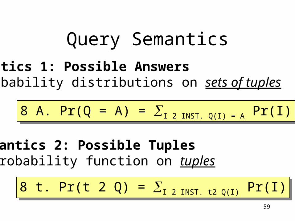
Query Semantics

Semantics 1: Possible AnswersA probability distributions on sets of tuples

8 A. Pr(Q = A) = I 2 INST. Q(I) = A Pr(I)8 A. Pr(Q = A) = I 2 INST. Q(I) = A Pr(I)

Semantics 2: Possible TuplesA probability function on tuples

8 t. Pr(t 2 Q) = I 2 INST. t2 Q(I) Pr(I)8 t. Pr(t 2 Q) = I 2 INST. t2 Q(I) Pr(I)

60

Example: Query SemanticsName City Product

John Seattle Gizmo

John Seattle Camera

Sue Denver Gizmo

Sue Denver Camera

Pr(I1) = 1/3

Name City Product

John Boston Gizmo

Sue Denver Gizmo

Sue Seattle Gadget

Name City Product

John Seattle Gizmo

John Seattle Camera

Sue Seattle Camera

Name City Product

John Boston Camera

Sue Seattle Camera

Pr(I2) = 1/12

Pr(I3) = 1/2

Pr(I4) = 1/12

SELECT DISTINCT x.productFROM Purchasep x, Purchasep yWHERE x.name = 'John' and x.product = y.product and y.name = 'Sue'

SELECT DISTINCT x.productFROM Purchasep x, Purchasep yWHERE x.name = 'John' and x.product = y.product and y.name = 'Sue'

Possible answers semantics:Answer set Probability

Gizmo, Camera 1/3 Pr(I1)

Gizmo 1/12 Pr(I2)

Camera 7/12 P(I3) + P(I4)

Tuple Probability

Camera 11/12 Pr(I1)+P(I3) + P(I4)

Gizmo 5/12 Pr(I1)+Pr(I2)

Possible tuples semantics:

PurchasepPurchasep

61

Special Case

Pr(I) = t 2 I pr(t) £ t I (1-pr(t))Pr(I) = t 2 I pr(t) £ t I (1-pr(t))

No restrictionspr : TUP ! [0,1]pr : TUP ! [0,1]

Tuple independent probabilistic database

INST = P(TUP)N = 2M

TUP = {t1, t2, …, tM}TUP = {t1, t2, …, tM} = all tuples

62

Tuple Prob. ) Possible WorldsName City pr

John Seattle p1 = 0.8

Sue Boston p2 = 0.6

Fred Boston p3 = 0.9Ip = Name City

John Seattl

Sue Bosto

Fred Bosto

Name City

Sue Bosto

Fred Bosto

Name City

John Seattl

Fred Bosto

Name City

John Seattl

Sue Bosto

Name City

Fred Bosto

Name City

Sue Bosto

Name City

John Seattl;

I1

(1-p1)(1-p2)(1-p3)

I2

p1(1-p2)(1-p3)

I3

(1-p1)p2(1-p3)

I4

(1-p1)(1-p2)p3

I5

p1p2(1-p3)

I6

p1(1-p2)p3

I7

(1-p1)p2p3

I8

p1p2p3

= 1

J = E[ size(Ip) ] =

2.3 tuples

63

Tuple Prob. ) Query Evaluation

Name City pr

John Seattle p1

Sue Boston p2

Fred Boston p3

Customer Product Date pr

John Gizmo . . . q1

John Gadget . . . q2

John Gadget . . . q3

Sue Camera . . . q4

Sue Gadget . . . q5

Sue Gadget . . . q6

Fred Gadget . . . q7

SELECT DISTINCT x.cityFROM Person x, Purchase yWHERE x.Name = y.Customer and y.Product = ‘Gadget’

SELECT DISTINCT x.cityFROM Person x, Purchase yWHERE x.Name = y.Customer and y.Product = ‘Gadget’

Tuple Probability

Seattle

Boston

1-(1-q2)(1-q3)p1( )

1- (1- ) £(1 - )

p2( )1-(1-q5)(1-q6)p3 q7

64

Summary of Part II

Possible Worlds Semantics

• Very powerful model: any tuple correlations

• Needs separate representation formalism

65

Summary of Part II

Query semantics

• Very powerful: every SQL query has semantics

• Very intuitive: from standard semantics

• Two variations, both appear in the literature

66

Summary of Part II

Possible answers semantics• Precise• Can be used to compose queries• Difficult user interface

Possible tuples semantics• Less precise, but simple; sufficient for most apps• Cannot be used to compose queries• Simple user interface

67

After the Break

Part III: Representation Formalisms

Part IV: Foundations

Part V: Algorithms, implementation techniques

Conclusions and Challenges

68

Part III

Representation Formalisms

69

Representation Formalisms

ProblemNeed a good representation formalism

• Will be interpreted as possible worlds

• Several formalisms exists, but no winner

Main open problem in probabilistic dbMain open problem in probabilistic db

70

Evaluation of Formalisms

• What possible worlds can it represent ?

• What probability distributions on worlds ?

• Is it closed under query application ?

71

Outline

A complete formalism:

• Intensional Databases

Incomplete formalisms:

• Various expressibility/complexity tradeoffs

72

Intensional Database

[Fuhr&Roellke:1997]

Atomic event idsAtomic event ids

Intensional probabilistic database J: each tuple t has an event attribute t.E

e1, e2, e3, …

p1, p2, p3, … 2 [0,1]

e3 Æ (e5 Ç : e2)

Probabilities: Probabilities:

Event expressions: Æ, Ç, :Event expressions: Æ, Ç, :

73

Intensional DB ) Possible WorldsName Address E

John Seattle e1 Æ (e2 Ç e3)

Sue Denver (e1 Æ e2 ) Ç (e2 Æ e3 )

J =

Ip

e1e2e3= 000 001 010 011 100 101 110 111

John Seattle

Sue Denver

John Seattle Sue Denver;

(1-p1)(1-p2)(1-p3)+(1-p1)(1-p2)p3

+(1-p1)p2(1-p3)+p1(1-p2)(1-p3

p1(1-p2) p3 (1-p1)p2 p3

p1p2(1-p3)+p1p2p3

74

Possible Worlds ) Intensional DB

Name Address E

John Seattle E1 Ç E2

John Boston E1 Ç E4

Sue Seattle E1 Ç E2 Ç E3

E1 = e1

E2 = :e1 Æ e2

E3 = :e1 Æ :e2 Æ e3

E4 = :e1 Æ :e2 Æ :e3 Æ e4“Prefix code”

Pr(e1) = p1

Pr(e2) = p2/(1-p1)Pr(e3) = p3/(1-p1-p2)Pr(e4) = p4 /(1-p1-p2-p3)

J =

Intesional DBs are completeIntesional DBs are complete

Name Address

John Seattle

John Boston

Sue Seattle

Name Address

John Seattle

Sue Seattle

Name Address

Sue Seattle

Name Address

John Boston

p1

p2

p3

p4

=Ip

75

Closure Under Operators

v E

v E

£

v1 E1

v1 v2 E1 Æ E2

v2 E2

v E1

v E2

… …

v E1 Ç E2 Ç . .

One still needs to compute probability of event expressionOne still needs to compute probability of event expression

[Fuhr&Roellke:1997]

-

v E1

v E1 Æ:E2

v E2

76

Summary on Intensional Databases

Event expression for each tuple• Possible worlds: any subset• Probability distribution: any

Complete (in some sense) … but impractical

Important abstraction: consider restrictions

Related to c-tables [Imilelinski&Lipski:1984]

77

Restricted Formalisms

Explicit tuples

• Have a tuple template for every tuple that may appear in a possible world

Implicit tuples

• Specify tuples indirectly, e.g. by indicating how many there are

78

Explicit Tuples

Independent tuples

Name City E pr

John Seattle e1 0.8

Sue Boston e2 0.2

Fred Boston e3 0.6

0

0independent

Atomic, distinct.May use TIDs.

E[ size(Customer) ] = 1.6 tuples

tuple = event

79

Application 1: Similarity PredicatesName City Profession

John Seattle statistician

Sue Boston musician

Fred Boston physicist

Cust Product Category

John Gizmo dishware

John Gadget instrument

John Gadget instrument

Sue Camera musicware

Sue Gadget microphone

Sue Gadget instrument

Fred Gadget microphone

SELECT DISTINCT x.cityFROM Person x, Purchase yWHERE x.Name = y.Cust and y.Product = ‘Gadget’ and x.profession ~ ‘scientist’ and y.category ~ ‘music’

SELECT DISTINCT x.cityFROM Person x, Purchase yWHERE x.Name = y.Cust and y.Product = ‘Gadget’ and x.profession ~ ‘scientist’ and y.category ~ ‘music’

Step 1:evaluate ~ predicates

80

Application 1: Similarity PredicatesName City Profession pr

John Seattle statistician p1=0.8

Sue Boston musician p2=0.2

Fred Boston physicist p3=0.9

Cust Product Category pr

John Gizmo dishware q1=0.2

John Gadget instrument q2=0.6

John Gadget instrument q3=0.6

Sue Camera musicware q4=0.9

Sue Gadget microphone q5=0.7

Sue Gadget instrument q6=0.6

Fred Gadget microphone q7=0.7SELECT DISTINCT x.cityFROM Personp x, Purchasep yWHERE x.Name = y.Cust and y.Product = ‘Gadget’ and x.profession ~ ‘scientist’ and y.category ~ ‘music’

SELECT DISTINCT x.cityFROM Personp x, Purchasep yWHERE x.Name = y.Cust and y.Product = ‘Gadget’ and x.profession ~ ‘scientist’ and y.category ~ ‘music’

Tuple Probability

Seattle p1(1-(1-q2)(1-q3))

Boston1-(1-p2(1-(1-q5)(1-q6))) £(1-p3q7)

Step 1:evaluate ~ predicates

Step 2:evaluate rest

of query

81

Explicit TuplesIndependent/disjoint tuples

Independent events: e1, e2, …, ei, …

Split ei into disjoint “shares” ei = ei1Ç ei2Ç ei3Ç…

e34, e37 ) disjoint events

e37, e57 ) independent events

--

0

82

Application 2: Inconsistent DataName City Product

John Seattle Gizmo

John Seattle Camera

John Boston Gadget

John Huston Gizmo

Sue Denver Gizmo

Sue Seattle Camera

Name ! City (violated)

SELECT DISTINCT ProductFROM CustomerWHERE City = ‘Seattle’

SELECT DISTINCT ProductFROM CustomerWHERE City = ‘Seattle’

Step 1:resolve violations

83

Application 2: Inconsistent DataName City Product E Pr

John Seattle Gizmo e11 1/3

John Seattle Camera e11 1/3

John Boston Gadget e12 1/3

John Huston Gizmo e13 1/3

Sue Denver Gizmo e21 1/2

Sue Seattle Camera e22 1/2

SELECT DISTINCT ProductFROM Customerp

WHERE City = ‘Seattle’

SELECT DISTINCT ProductFROM Customerp

WHERE City = ‘Seattle’

++

--

0

Tuple Probability

Gizmo p11 = 1/3

Camera 1-(1-p11)(1-p22) = 2/3

Step 1:resolve violations

Step 2:evaluate query

E[ size(Customer) ] = 2 tuples

84

Inaccurate Attribute Values

[Barbara et al.92, Lakshmanan et al.97,Ross et al.05;Widom05]

Name Dept Bonus

John Toy

Great 0.4

Good 0.5

Fair 0.1

Fred Sales Good 1.0

Name Dept Bonus E Pr

John Toy Great e11 0.4

John Toy Good e12 0.5

John Toy Fair e13 0.1

Fred Sales Good e21 1.0

Inaccurate attributes Disjoint and/or independentevents

85

Summary on Explicit Tuples

Independent or disjoint/independent tuples• Possible worlds: subsets• Probability distribution: restricted• Closure: no

In KR:• Bayesian networks: disjoint tuples• Probabilistic relational models: correlated tuples

[Friedman,Getoor,Koller,Pfeffer:1999]

86

Implicit Tuples

[Mendelzon&Mihaila:2001,Widom:2005,Miklau&S04,Dalvi et al.05]

“There are other, unknown tuples out there”

Name City Profession

John Seattle statistician

Sue Boston musician

Fred Boston Physicist

Covers 10%

30 other tuples

Completeness =10%

or

87

Implicit Tuples

Name Depart Phone

C tuples(e.g. C = 30)

[Miklau,Dalvi&S:2005,Dalvi&S:2005]

Statistics based:

EmployeeEmployeeSemantics 1:

size(Employee)=C

Semantics 2:E[size(Employee)]=C

We go with #2: the expected size is CWe go with #2: the expected size is C

88

Implicit Possible Tuples

Employee(name, dept, phone)Employee(name, dept, phone)

E[ Size(Employee) ] = CE[ Size(Employee) ] = C

n1 = | Dname|n2 = | Ddept|n3 = | Dphone|

8 t. Pr(t) = C / (n1 n2 n3)8 t. Pr(t) = C / (n1 n2 n3)

[Miklau,Dalvi&S:2005,Dalvi&S:2005]

Binomial distribution

89

S :- Employee(“Mary”, -, 5551234)S :- Employee(“Mary”, -, 5551234) Pr(S) C/n1n3Pr(S) C/n1n3

V1 :- Employee(“Mary”, “Sales”, -)V1 :- Employee(“Mary”, “Sales”, -)

Pr(SV1) C/n1n2n3

Pr(V1) C/n1n2

Pr(S | V1) 1/ n3Pr(S | V1) 1/ n3

V2 :- Employee(-, “Sales”, 5551234)V2 :- Employee(-, “Sales”, 5551234)

Pr(SV1V2) C/n1n2n3

Pr(V1 V2) C/n1n2 n3

Pr(S | V1V2) 1Pr(S | V1V2) 1

Pr(name,dept,phone) = C / (n1 n2 n3)Pr(name,dept,phone) = C / (n1 n2 n3)

Practical secrecy

Leakage

Application 3: Information Leakage

[Miklau,Dalvi&S:2005]

90

Summary on Implicit Tuples

Given by expected cardinality• Possible worlds: any• Probability distribution: binomial

May be used in conjunction with other formalisms• Entropy maximization

Conditional probabilities become important

[Domingos&Richardson:2004,Dalvi&S:2005]

91

Summary on Part III: Representation Formalism

• Intensional databases: – Complete (in some sense)– Impractical, but…– …important practical restrictions

• Incomplete formalisms:– Explicit tuples– Implicit tuples

• We have not discussed query processing yet

92

Part IV

Foundations

93

Outline

• Probability of boolean expressions

• Query probability

• Random graphs

94

Probability of Boolean Expressions

E = X1X3 Ç X1X4 Ç X2X5 Ç X2X6E = X1X3 Ç X1X4 Ç X2X5 Ç X2X6

Randomly make each variable true with the following probabilities

Pr(X1) = p1, Pr(X2) = p2, . . . . . , Pr(X6) = p6

What is Pr(E) ???What is Pr(E) ???

Answer: re-group cleverly E = X1 (X3 Ç X4 ) Ç X2 (X5 Ç X6)E = X1 (X3 Ç X4 ) Ç X2 (X5 Ç X6)

Pr(E)=1 - (1-p1(1-(1-p3)(1-p4))) (1-p2(1-(1-p5)(1-p6)))

Pr(E)=1 - (1-p1(1-(1-p3)(1-p4))) (1-p2(1-(1-p5)(1-p6)))

Needed for query processing

95

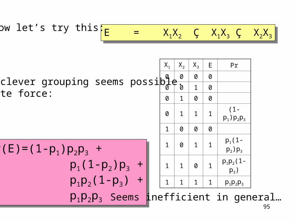
E = X1X2 Ç X1X3 Ç X2X3E = X1X2 Ç X1X3 Ç X2X3

Pr(E)=(1-p1)p2p3 + p1(1-p2)p3 + p1p2(1-p3) + p1p2p3

Pr(E)=(1-p1)p2p3 + p1(1-p2)p3 + p1p2(1-p3) + p1p2p3

Now let’s try this:

No clever grouping seems possible.Brute force:

X1 X2 X3 E Pr

0 0 0 0

0 0 1 0

0 1 0 0

0 1 1 1 (1-p1)p2p3

1 0 0 0

1 0 1 1 p1(1-p2)p3

1 1 0 1 p1p2(1-p3)

1 1 1 1 p1p2p3

Seems inefficient in general…

96

Complexity of Boolean Expression Probability

Theorem [Valiant:1979]For a boolean expression E, computing Pr(E) is #P-complete

Theorem [Valiant:1979]For a boolean expression E, computing Pr(E) is #P-complete

NP = class of problems of the form “is there a witness ?” SAT#P = class of problems of the form “how many witnesses ?” #SAT

The decision problem for 2CNF is in PTIMEThe counting problem for 2CNF is #P-complete

[Valiant:1979]

97

Summary on Boolean Expression Probability

• #P-complete

• It’s hard even in simple cases: 2DNF

• Can do Monte Carlo simulation (later)

98

Query Complexity

Data complexity of a query Q:

• Compute Q(Ip), for probabilistic database Ip

Simplest scenario only:

• Possible tuples semantics for Q

• Independent tuples for Ip

99

or: p1 + p2 + …

Extensional Query EvaluationRelational ops compute probabilities

v p

v p

£

v1 p1

v1 v2 p1 p2

v2 p2

v p1

v p2

v 1-(1-p1)(1-p2)…

[Fuhr&Roellke:1997,Dalvi&S:2004]

-

v p1

v p1(1-p2)

v p2

Data complexity: PTIMEData complexity: PTIME

100

Jon Sea p1

Jon q1

Jon q2

Jon q3

SELECT DISTINCT x.CityFROM Personp x, Purchasep yWHERE x.Name = y.Cust and y.Product = ‘Gadget’

SELECT DISTINCT x.CityFROM Personp x, Purchasep yWHERE x.Name = y.Cust and y.Product = ‘Gadget’

Jon Sea p1q1

Jon Sea p1q2

Jon Sea p1q3

Sea 1-(1-p1q1)(1- p1q2)(1- p1q3)

£

Jon Sea p1

Jon q1

Jon q2

Jon q3

Jon 1-(1-q1)(1-q2)(1-q3)

£

Jon Sea p1(1-(1-q1)(1-q2)(1-q3))

[Dalvi&S:2004]

Wrong !

Correct

Depends on plan !!!Depends on plan !!!

101

Query Complexity

Sometimes @ correct extensional plan

Qbad :- R(x), S(x,y), T(y)Qbad :- R(x), S(x,y), T(y) Data complexityis #P complete

Theorem The following are equivalent• Q has PTIME data complexity• Q admits an extensional plan (and one finds it in PTIME)• Q does not have Qbad as a subquery

Theorem The following are equivalent• Q has PTIME data complexity• Q admits an extensional plan (and one finds it in PTIME)• Q does not have Qbad as a subquery

[Dalvi&S:2004]

102

Summary on Query Complexity

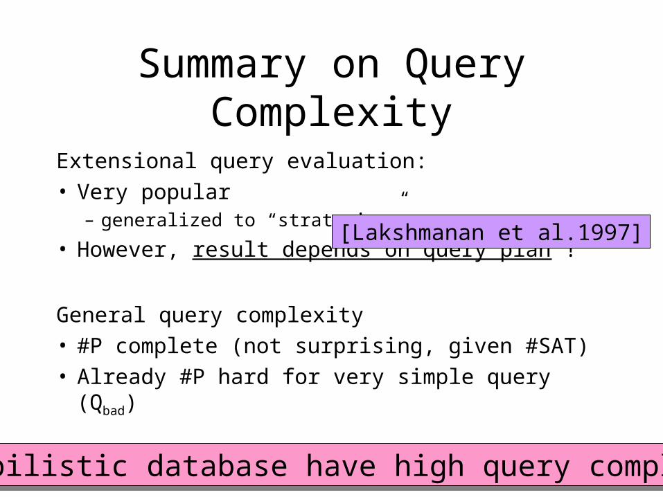
Extensional query evaluation:• Very popular

– generalized to “strategies”

• However, result depends on query plan !

General query complexity• #P complete (not surprising, given #SAT)

• Already #P hard for very simple query (Qbad)

Probabilistic database have high query complexityProbabilistic database have high query complexity

[Lakshmanan et al.1997]

103

Random Graphs

[Erdos&Reny:1959,Fagin:1976,Spencer:2001]

Domain:

Gp = tuple-independent

Boolean query Q What is limn! 1 Q(Gp)What is limn! 1 Q(Gp)

Relation:

Graph G:1

2

4

3 n

Random graph Gp

12

4

3 n

Edges hidinghere

G(x,y)G(x,y)

D={1,2, …, n}D={1,2, …, n}

pr(t1) = … pr(tM) = ppr(t1) = … pr(tM) = p

104

Fagin’s 0/1 Law

[Fagin:1976]

Let the tuple probability be p = 1/2

Theorem [Fagin:1976,Glebskii et al.1969]For every sentence Q in First Order Logic,limn! 1 Q(Gp) exists and is either 0 or 1

Theorem [Fagin:1976,Glebskii et al.1969]For every sentence Q in First Order Logic,limn! 1 Q(Gp) exists and is either 0 or 1

Holds almost surely: lim = 1 Does not hold a.s. lim = 0

8 x.9 y.G(x,y) 9 x.8y.G(x,y)

9 x.9 y.9 z. G(x,y)ÆG(y,z)ÆG(x,z)

8 x.8y. G(x,y)

Examples

105

Erdos and Reny’s Random Graphs

[Erdos&Reny:1959]

Now let p = p(n) be a function of n

Theorem [Erdos&Ren]y:1959]For any monotone Q, 9 a threshold function t(n) s.t.:

if p(n) ¿ t(n) then limn! 1Q(Gp)=0if p(n) À t(n) then limn! 1Q(Gp)=1

Theorem [Erdos&Ren]y:1959]For any monotone Q, 9 a threshold function t(n) s.t.:

if p(n) ¿ t(n) then limn! 1Q(Gp)=0if p(n) À t(n) then limn! 1Q(Gp)=1

106

The Evoluation of Random Graphs

[Erdos&Reny:1959; Spencer:2001]

The tuple probability p(n) “grows” from 0 to 1.How does the random graph evolve ?

The tuple probability p(n) “grows” from 0 to 1.How does the random graph evolve ?

Remark: C(n) = E[ Size(G) ] ' n2p(n)

The expected size C(n) “grows” from 0 to n2.How does the random graph evolve ?

The expected size C(n) “grows” from 0 to n2.How does the random graph evolve ?

0 … 1

107

Contains almost surely Does not contain almost surely

(nothing)

The Void

p(n) ¿ 1/n2p(n) ¿ 1/n2 C(n) ¿ 1 C(n) ¿ 1

The graph is empty 0/1 Law holds

[Spencer:2001]

108

Contains almost surely Does not contain almost surely

trees with · k edges trees > k edges

cycles

On the k’th Day

1/n1+1/(k-1) ¿ p(n) ¿ 1/n1+1/k1/n1+1/(k-1) ¿ p(n) ¿ 1/n1+1/kn1-1/(k-1) ¿ C(n) ¿ n1-1/kn1-1/(k-1) ¿ C(n) ¿ n1-1/k

The graph is disconnected 0/1 Law holds

[Spencer:2001]

109

On Day 1/n1+ ¿ p(n) ¿ 1/n, 8 1/n1+ ¿ p(n) ¿ 1/n, 8 n1- ¿ C(n) ¿ n, 8 n1- ¿ C(n) ¿ n, 8

The graph is disconnected 0/1 Law holds

[Spencer:2001]

Contains almost surely Does not contain almost surely

Any Tree cycles

110

Past the Double Jump (1/n)1/n ¿ p(n) ¿ ln(n)/n1/n ¿ p(n) ¿ ln(n)/n n ¿ C(n) ¿ n ln(n)n ¿ C(n) ¿ n ln(n)

The graph is disconnected 0/1 Law holds

[Spencer:2001]

Contains almost surely Does not contain almost surely

Any Tree

Any Cycle

Any subgraph with k nodes and ¸ k+1 edges

111

Past Connectivity

ln(n)/n ¿ p(n) ¿ 1/n1-, 8 ln(n)/n ¿ p(n) ¿ 1/n1-, 8 n ln(n) ¿ C(n) ¿ n1+, 8 n ln(n) ¿ C(n) ¿ n1+, 8

The graph is connected ! 0/1 Law holds

Strange logicof random graphs !!

[Spencer:2001]

Contains almost surely Does not contain almost surely

Every node has degree ¸ k,for every k ¸ 0

Any subgraph with k nodes and ¸ k+1 edges

112

Big Graphs

p(n) = 1/n, 2 (0,1)p(n) = 1/n, 2 (0,1) C(n) = n2-, 2 (0,1)C(n) = n2-, 2 (0,1)

0/1 Law holds is irrational )

is rational ) 0/1 Law does not hold

[Spencer:2001]

Fagin’s framework: = 0

p(n) = O(1)p(n) = O(1) C(n) = O(n2)C(n) = O(n2)

0/1 Law holds

113

Summary on Random Graphs

• Very rich field– Over 700 references in [Bollobas:2001]

• Fascinating theory– Evening reading: the evolution of random

graphs (e.g. from [Spencer:2001])

114

Summary on Random Graphs

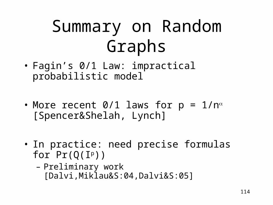
• Fagin’s 0/1 Law: impractical probabilistic model

• More recent 0/1 laws for p = 1/n [Spencer&Shelah, Lynch]

• In practice: need precise formulas for Pr(Q(Ip))– Preliminary work [Dalvi,Miklau&S:04,Dalvi&S:05]

115

Part V

Algorithms,Implementation Techniques

116

Query Processing on a Probabilistic Database

Probabilisticdatabase

SQL QuerySQL Query ProbabilisticQuery engine

Top k answers

1. Simulation

2. Extensional joins

3. Indexes

117

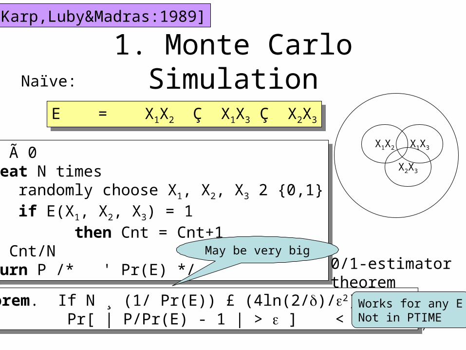
1. Monte Carlo Simulation

[Karp,Luby&Madras:1989]

E = X1X2 Ç X1X3 Ç X2X3E = X1X2 Ç X1X3 Ç X2X3

Cnt à 0repeat N times randomly choose X1, X2, X3 2 {0,1} if E(X1, X2, X3) = 1 then Cnt = Cnt+1P = Cnt/Nreturn P /* ' Pr(E) */

Cnt à 0repeat N times randomly choose X1, X2, X3 2 {0,1} if E(X1, X2, X3) = 1 then Cnt = Cnt+1P = Cnt/Nreturn P /* ' Pr(E) */

Theorem. If N ¸ (1/ Pr(E)) £ (4ln(2/)/2) then: Pr[ | P/Pr(E) - 1 | > ] <

Theorem. If N ¸ (1/ Pr(E)) £ (4ln(2/)/2) then: Pr[ | P/Pr(E) - 1 | > ] <

May be very big

X1X2 X1X3

X2X3

Naïve:

0/1-estimatortheorem

Works for any ENot in PTIME

118

Monte Carlo Simulation

[Karp,Luby&Madras:1989]

Cnt à 0; S à Pr(C1) + … + Pr(Cm);repeat N times randomly choose i 2 {1,2,…, m}, with prob. Pr(Ci) / S randomly choose X1, …, Xn 2 {0,1} s.t. Ci = 1 if C1=0 and C2=0 and … and Ci-1 = 0 then Cnt = Cnt+1P = Cnt/N * 1/return P /* ' Pr(E) */

Cnt à 0; S à Pr(C1) + … + Pr(Cm);repeat N times randomly choose i 2 {1,2,…, m}, with prob. Pr(Ci) / S randomly choose X1, …, Xn 2 {0,1} s.t. Ci = 1 if C1=0 and C2=0 and … and Ci-1 = 0 then Cnt = Cnt+1P = Cnt/N * 1/return P /* ' Pr(E) */

Theorem. If N ¸ (1/ m) £ (4ln(2/)/2) then: Pr[ | P/Pr(E) - 1 | > ] <

Theorem. If N ¸ (1/ m) £ (4ln(2/)/2) then: Pr[ | P/Pr(E) - 1 | > ] <

E = C1 Ç C2 Ç . . . Ç CmE = C1 Ç C2 Ç . . . Ç Cm

Improved:

Now it’s better

Only for E in DNFIn PTIME

119

Summary on Monte Carlo

Some form of simulation is needed in probabilistic databases, to cope with the #P-hardness bottleneck

• Naïve MC: works well when Prob is big

• Improved MC: needed when Prob is small

120

2. The Threshold Algorithm

Problem: SELECT *

FROM Rp, Sp, Tp

WHERE Rp.A = Sp.B and Sp.C = Tp.D

SELECT *FROM Rp, Sp, Tp

WHERE Rp.A = Sp.B and Sp.C = Tp.D

Have subplans for Rp, Sp, Tp returning tuples sorted by their probabilities x, y, z

Score combination:f(x, y, z) = xyz

How do we compute the top-k matching records ?How do we compute the top-k matching records ?

[Nepal&Ramakrishna:1999,Fagin,Lotem,Naor:2001; 2003]

121

[Fagin,Lotem,Naor:2001; 2003]

“No Random Access” (NRA)

H32 x1

H5555 x2

H007 x3

? ?

. . .

1 ¸ x1 ¸ x2 ¸ …

H5555 y1

H44 y2

H999 y3

? ?

. . .

1 ¸ y1 ¸ y2 ¸ …

H44 z1

H007 z2

H5555 z3

? ?

. . .

1 ¸ z1 ¸ z2 ¸ …

H5555:f(x2,y1,z3)

H007:f(x3,?, z2)

H???:f(?, ?, ?)

H32:f(x1,?, ?)

H999:f(?, y3, ?)

0 · ? · y3

Total score:

Rp= Sp= Tp=

122

[Fagin,Lotem,Naor:2001; 2003]

Termination condition:

H???:f(?, ?, ?)

k objects:Guaranteed to be top-k

Threshold score

The algorithm is “instance optimal”strongest form of optimality

123

Summary on the Threshold Algorithm

• Simple, intuitive, powerful

• There are several variations: see paper

• Extensions:– Use probabilistic methods to estimate the

bounds more aggressively

– Distributed environment

[Theobald,Weikum&Schenkel:2004]

[Michel, Triantafillou&Weikum:2005]

124

Approximate String Joins

[Gravano et al.:2001]

Problem: SELECT *FROM R, SWHERE R.A ~ S.B

SELECT *FROM R, SWHERE R.A ~ S.B

Simplification for this tutorial: A ~ B means “A, B have at least k q-grams in common”

125

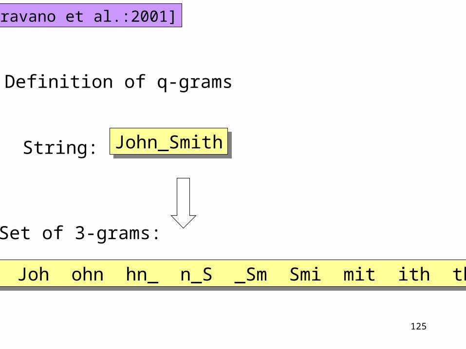
[Gravano et al.:2001]

Definition of q-grams

John_SmithJohn_Smith

##J #Jo Joh ohn hn_ n_S _Sm Smi mit ith th# h####J #Jo Joh ohn hn_ n_S _Sm Smi mit ith th# h##

String:

Set of 3-grams:

126

[Gravano et al.:2001]

SELECT *FROM R, SWHERE R.A ~ S.B

SELECT *FROM R, SWHERE R.A ~ S.B

SELECT *FROM R, SWHERE common_grams(R.A, S.B) ¸ k

SELECT *FROM R, SWHERE common_grams(R.A, S.B) ¸ k

Naïve solution,using UDF(user defined function)

127

A q-gram index:

Key A …

…

k743 John_Smith …

…

R

Key G

…

k743 ##J

k743 #Jo

k743 Joh

…

RAQ

[Gravano et al.:2001]

128

[Gravano et al.:2001]

SELECT *FROM R, SWHERE R.A ~ S.B

SELECT *FROM R, SWHERE R.A ~ S.B

SELECT R.*, S.*FROM R, RAQ, S, SBQWHERE R.Key = RAQ.Key and S.Key=SBQ.Key and RAQ.G = RBQ.GGROUP BY RAQ.Key, RBQ.KeyHAVING count(*) ¸ k

SELECT R.*, S.*FROM R, RAQ, S, SBQWHERE R.Key = RAQ.Key and S.Key=SBQ.Key and RAQ.G = RBQ.GGROUP BY RAQ.Key, RBQ.KeyHAVING count(*) ¸ k

Solution usingthe Q-gram Index

129

Summary on Part V:Algorithms

A wide range of disparate techniques

• Monte Carlo Simulations (also: MCMC)

• Optimal aggregation algorithms (TA)

• Efficient engineering techniques

Needed: unified framework for efficient query evaluation in probabilistic databases

130

Conclusions andChallenges Ahead

131

Conclusions

Imprecisions in data:

• A wide variety of types have specialized management solutions

• Probabilistic databases promise uniform framework, but require full complexity

132

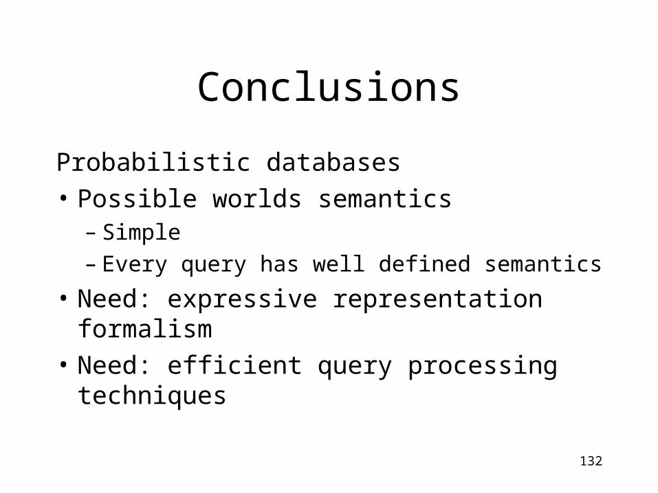
Conclusions

Probabilistic databases

• Possible worlds semantics– Simple– Every query has well defined semantics

• Need: expressive representation formalism

• Need: efficient query processing techniques

133

Challenge 1: Specification Frameworks

The Goal:

• Design framework that is usable, expressive, efficient

The Challenge

• Tradeoff between expressibility and tractability

134

Challenge 1: Specification Frameworks

Features to have:• Support probabilistic statements:

– Simple: (Fred, Seattle, Gizmo) 2 Purchase has probability 60%

– Complex: “Fred and Sue live in the same city” has probability 80%

• Support tuple corrleations– “t1 and t2 are correlated positively 30%”

• Statistics statements:– There are about 2000 tuples in Purchase

– There are about 100 distinct Cities

– Every customer buys about 4 products

[Domingos&Richardson:04,Sarma,Benjelloun,Halevy,Widom:2005]

135

Challenge 2:Query Evaluation

Complexity• Old: = f(query-language)• New: = f(query-language, specification-language)

Exact algorithm: #P-complete in simple cases

Challenge: characterize the complexity of approximation algorithms

136

Challenge 2:Query Evaluation

Implementations:• Disparate techniques require unified framework• Simulation:

– Client side or server side ?– How to schedule simulation steps ?– How to push simulation steps in relational operators ?– How to compute subplans extensionally, when possible ?

• Top-k pruning:– How can we “push thresholds” down the query plan ?

137

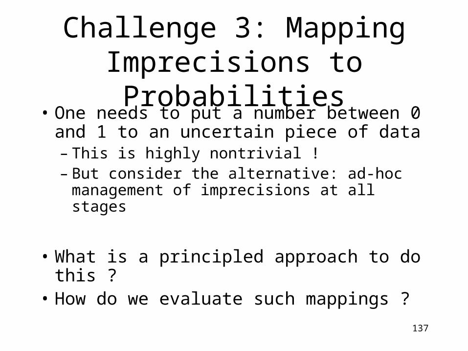
Challenge 3: Mapping Imprecisions to Probabilities

• One needs to put a number between 0 and 1 to an uncertain piece of data– This is highly nontrivial !– But consider the alternative: ad-hoc

management of imprecisions at all stages

• What is a principled approach to do this ?• How do we evaluate such mappings ?

138

The Endp

Questions ?