1: Elements of Statistical Signal ProcessingECE 830, Spring 2017

1 / 31

What do we have here?

The first step in many scientific and engineering problems is oftensignal analysis. Given measurements or observations of somephysical process, we ask the simple question “what do we havehere?” For instance,

I Is there any information in my measurements, or are they justnoise?

I Is my signal in category A or B?

I What is the signal underlying my noisy measurements?

Answering this question can be particularly challenging when

I measurements are corrupted by noise or errors

I the physical process is“transient” or its behavior changes overtime.

2 / 31

Fourier analysis

In some contexts, these challenges can be addressed via Fourieranalysis, one of the major achievements in physics andmathematics. It is central to signal theory and processing forseveral reasons.Recall the Fourier series:

x(t) =

∞∑k=−∞

cke−j2πfkt.

This is used for

I analysis of physical waves (acoustics, vibrations, geophysics,optics)

I analysis of periodic processes (economics, biology, astronomy)

3 / 31

Fourier analysis and filteringRecall the Fourier transform

X(f) =

∫ ∞−∞

x(t)e−j2πftdt

and the convolution integral

y(t) =

∫ ∞−∞

h(τ)x(t− τ)dτ

=

∫ ∞−∞

H(f)X(f)ej2πftdf

which describes, for example, the result of sending a signal xthrough a filter h. Two key facts:

I Convolution in time ⇐⇒ multiplication in frequency

I A stationary, zero-mean, Gaussian random process can berepresented as a white noise process passed through a linear,time-invariant filter

4 / 31

Limitations of Fourier analysis

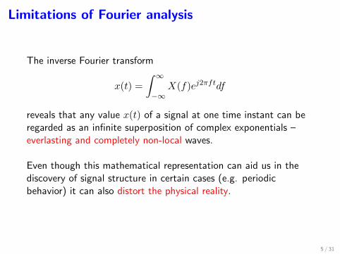
The inverse Fourier transform

x(t) =

∫ ∞−∞

X(f)ej2πftdf

reveals that any value x(t) of a signal at one time instant can beregarded as an infinite superposition of complex exponentials –everlasting and completely non-local waves.

Even though this mathematical representation can aid us in thediscovery of signal structure in certain cases (e.g. periodicbehavior) it can also distort the physical reality.

5 / 31

In particular...

1. Many signals, especially those which are transient in nature,are not well represented in terms of sinusoidal waves.

I e.g. Images contain edges which are not efficiently representedwith sinusoids.

I e.g. Suppose that the signal x(t) is exactly zero outside acertain time interval (e.g. by switching a machine on and off).

Although this signal can still be studied by Fourier techniques,the frequency domain representation has a very artificialbehavior. The time signal’s zero values are achieved by aninfinite superposition of virtual waves that interfere in such away that they cancel each other out.

6 / 31

In particular...

2. often, it is the non-stationary or transient components of asignal that carry the important information.

e.g. Imagine that you are on a beach, watching the waves rollin to shore. Your peaceful state is broken as dolphins begin toevacuate earth to make way for an intergalactic superhighway.

7 / 31

In particular...

3. As we have seen, stationaryGaussian processes areintimately linked withFourier analysis. However,many signals in which weare interested (e.g. speech,images) are not wellmodeled as stationary andGaussian

8 / 31

In this course, we will move beyond Fourier analysis and focus on

Statistical Digital Signal Processing

Statistical based on probabilistic models for signals and noise

Digital discrete-time, sampled, quantized

Signal waveform, sequence of measurements or observations

Processing analyze, modify, synthesize

Examples of digital signals

I sampled speech waveform

I pixelized image

I Dow-Jones index

I stream of internet packets

I vector of medical predictors

9 / 31

A major difficultyIn many DSP applications, we don’t have complete or perfectknowledge of the signals we wish to precess. We are faced withmany unknowns and uncertainties.Examples:

I Unknown signal parameters (delay of radar return, pitch ofspeech signal)

I Environmental noise (multipath signals in wirelesscommunications, ambient electromagnetic waves, radarjamming)

I Sensor noise (grainy images, old phonograph recordings)

I Variability inherent in nature (stock market, internet)

How can we process signals in the face of such uncertainty? Canwe model the uncertainty and incorporate this model into theprocessing?Statistical Signal Processing is the study of answers to these

questions.10 / 31

Modeling uncertainty

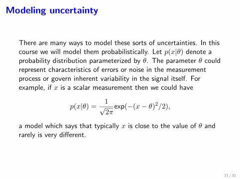
There are many ways to model these sorts of uncertainties. In thiscourse we will model them probabilistically. Let p(x|θ) denote aprobability distribution parameterized by θ. The parameter θ couldrepresent characteristics of errors or noise in the measurementprocess or govern inherent variability in the signal itself. Forexample, if x is a scalar measurement then we could have

p(x|θ) = 1√2π

exp(−(x− θ)2/2),

a model which says that typically x is close to the value of θ andrarely is very different.

11 / 31

Why Probabilistic Models?

The observations or measurements we make are seldom perfect;often they are impure and contaminated by effects unknown to us.We call these effects noise. Our models are seldom perfect. Eventhe best choice of θ may not perfectly predict new observations.We call these modeling errors bias.

How do we model noise and bias, these uncertain errors? We needa calculus for uncertainty, and among many that have beenproposed and used, the probabilistic framework appears to be themost successful, and in many situations it is physically plausible aswell.

12 / 31

Uses of probabilistic models

I sensor noise modeled as an additive Gaussian random variable

I uncertainty in the phase of a sinusoidal signal modeled as auniform random variable on [0, 2π)

I uncertainty in the number of photons striking a CCD per unittime modeled as a Poisson random variable.

13 / 31

Components of Statistical Signal Processing:Modeling, Measurement, and Inference

Step 1: Postulate a probability model (or collection of models) thatcan be expected to reasonably capture the uncertainties in thedata

Step 2: Collect data.

Step 3: Formulate statistics that allow us to interpret or understandour probability models.

14 / 31

Probability and statistics

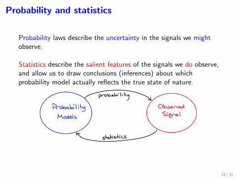
Probability laws describe the uncertainty in the signals we mightobserve.

Statistics describe the salient features of the signals we do observe,and allow us to draw conclusions (inferences) about whichprobability model actually reflects the true state of nature.

15 / 31

Statistics

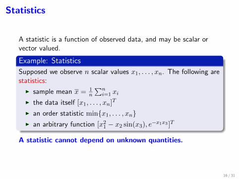
A statistic is a function of observed data, and may be scalar orvector valued.

Example: Statistics

Supposed we observe n scalar values x1, . . . , xn. The following arestatistics:

I sample mean x = 1n

∑ni=1 xi

I the data itself [x1, . . . , xn]T

I an order statistic min{x1, . . . , xn}I an arbitrary function [x21 − x2 sin(x3), e−x1x3 ]T

A statistic cannot depend on unknown quantities.

16 / 31

Four main problems

There are four fundamental inference problems in statistical signalprocessing that will be the focus of this course.

Example: Detection

Suppose that θ takes one of two possible values, so that eitherp(x|θ1) or p(x|θ2) fit the data x the best. Then we need to“decide” whether p(x|θ1) is a better model than p(x|θ2). Moregenerally, θ may be one of a finite number of values {θ1, . . . , θM}and we must decide among the M models.

17 / 31

A Detection Example

Consider a binary communication system. Let s = [s1, . . . , sn]denote a digitized waveform. A transmitter communicates a bit ofinformation by sending s or −s (for 1 or 0, respectively). Thereceiver measures a noisy version of the transmitted signal.

0 0.2 0.4 0.6 0.8 1−6

−4

−2

0

2

4

6

8

10

i

datas−s

18 / 31

A detection example (cont.)

We model our observations as

xi = θsi + εi , i = 1, . . . , n

The parameter θ is either +1 or −1, depending on which bit thetransmitter is sending. The {εi} represent errors incurred duringthe transmission process. So we have two models, or hypotheses,for the data:

H0 : xi = +si + εi , i = 1, . . . , n

H1 : xi = −si + εi , i = 1, . . . , n

How well does {si} match {xi}? How well does {−si} match{xi}?

19 / 31

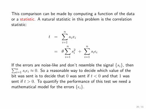
This comparison can be made by computing a function of the dataor a statistic. A natural statistic in this problem is the correlationstatistic:

t =

n∑i=1

sixi

= θ

n∑i=1

s2i +

n∑i=1

siεi

If the errors are noise-like and don’t resemble the signal {si}, then∑ni=1 siεi ≈ 0. So a reasonable way to decide which value of the

bit was sent is to decide that 0 was sent if t < 0 and that 1 wassent if t > 0. To quantify the performance of this test we need amathematical model for the errors {εi}.

20 / 31

Four main problems

Example: Parameter Estimation

Suppose that θ belongs to an infinite set. Then we must decide orchoose among an infinite number of models. In this sense,estimation may be viewed as an extension of detection to infinitemodel classes. This extension presents many new challenges andissues and so it is given its own name.

21 / 31

A Parameter Estimation Example

22 / 31

Four main problems

Example: Signal Estimation/Prediction

In many problems we wish to predict the value of a signal x givenan observation of another related signal y. We can model therelationship between x and y using a joint probability distribution,p(x, y). The conditional distribution of x given y, denoted byp(x|y), can be derived from the joint distribution and theprediction problem can then be viewed as determining a value of xthat is highly probable given y.

23 / 31

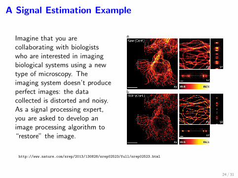
A Signal Estimation Example

Imagine that you arecollaborating with biologistswho are interested in imagingbiological systems using a newtype of microscopy. Theimaging system doesn’t produceperfect images: the datacollected is distorted and noisy.As a signal processing expert,you are asked to develop animage processing algorithm to“restore” the image.

http://www.nature.com/srep/2013/130828/srep02523/full/srep02523.html

24 / 31

A Signal Estimation Example (cont.)

Let us assume that the distortion is a linear operation. Then wecan model the collected data by the following equation.

y = Hx+ w

where

I x is the ideal image we wish to recover (represented as avector, each element of which is a pixel),

I H is a known model of the distortion (represented as amatrix), and

I w is a vector of noise.

25 / 31

A Signal Estimation Example (cont.)

It is tempting to ignore w and simply attempt to solve the systemof equations y = Hx for x. There are two problems with thisapproach.

1. The system of equations may not admit a unique solution,depending on the physics of the imaging system. If a uniquesolution exists, the problem is said to be well-posed, otherwiseit is called ill-posed.

2. Even if the system of equations is invertible, it may beill-conditioned, which means that small perturbations due tonoise and numerical methods can lead to large errors in therestoration of x.

26 / 31

Four main problems

Example: Learning

Sometimes we don’t know a good model the relationship betweenx and y, but we do have a number of “training examples”, say{xi, yi}ni=1, that give us some indication of the relationship. Thegoal of learning is to design a good prediction rule for y given xusing these examples, instead of p(y|x).

27 / 31

The Netflix problem

28 / 31

The Netflix prize

29 / 31

Example: Predicting Netflix ratings

Here x contains the measuredmovie ratings and y are theunknown movie ratings we wishto predict.

30 / 31

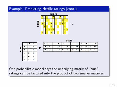
Example: Predicting Netflix ratings (cont.)

One probabilistic model says the underlying matrix of “true”ratings can be factored into the product of two smaller matrices.

31 / 31

Example: Predicting Netflix ratings (cont.)

One probabilistic model says the underlying matrix of “true”ratings can be factored into the product of two smaller matrices.

31 / 31