1 electron transfer reactions · 1 electron transfer reactions ophir snir and ira a. weinstock 1.1...

1 Electron Transfer Reactions

OPHIR SNIR and IRA A. WEINSTOCK

1.1 INTRODUCTION

Over the past few decades, applications of the Marcus model to inorganic electron

transfer reactions have become routine. Despite the many approximations needed

to simplify the theoretical descriptions to obtain a simple quadratic model, and the

assumptions then needed to apply this model to actual reactions, agreement between

calculated and observed rate constants is remarkably common. Because of this, the

Marcus model is widely used to assess the nature of electron transfer reactions. The

intent of this chapter is tomake this useful toolmore accessible to practicing chemists.

In that sense, it is written from a “reaction chemist’s”1 perspective. In 1987, Eberson

published an excellent monograph that provides considerable guidance in the context

of organic reactions.2 In addition to a greater focus on inorganic reactions, this chapter

covers electrolyte theory and ion pairing in more detail, and worked examples are

presented in a step-by-step fashion to guide the reader from theory to application.

The chapter begins with an introduction toMarcus’ theoretical treatment of outer-

sphere electron transfer. The emphasis is on communicating the main features of the

theory and on bridging the gap between theory and practically useful classicalmodels.

The chapter then includes an introduction to models for collision rates between

charged species in solution, and the effects on these of salts and ionic strength, which

all predated the Marcus model, but upon which it is an extension. Collision rate and

electrolyte models, such as those of Smoluchowski, Debye, H€uckel, and others, applyin ideal cases rarely met in practice. The assumptions of the models will be defined,

and the common situations in which real reacting systems fail to comply with them

will be highlighted. These models will be referred to extensively in the second half of

the chapter, where the conditions that must be met in order to use the Marcus model

properly, to avoid common pitfalls, and to evaluate situations where calculated values

fail to agree with experimental ones will be clarified.

Those who have taught themselves how to apply the Marcus model and cross-

relation correctly will appreciate the gap between the familiar “formulas” published

in numerous articles and texts and the assumptions, definitions of terms, and physical

Physical Inorganic Chemistry: Reactions, Processes, and Applications Edited by Andreja BakacCopyright � 2010 by John Wiley & Sons, Inc.

1

COPYRIG

HTED M

ATERIAL

constants needed to apply them. This chapter will fill that gap in the service of those

interested in applying the model to their own chemistry. In addition, the task of

choosing compatible units for physical constants and experimental variables will be

simplified through worked examples that include dimensional analysis.

Themanythousandsofarticlesonouter-sphereelectron transfer reactions involving

metal ions and their complexes cannot be properly reviewed in a single chapter. From

this substantial literature, however, instructive exampleswill be selected. Importantly,

they will be explaining in more detail than is typically found in review articles or

treatises on outer-sphere electron transfer. In fact, the analyses provided here are quite

different fromthose typically found in theprimaryarticles themselves.There, innearly

all cases, the objective is to present and discuss calculated results. Here, the goal is to

enable readers to carry out the calculations that lead to publishable results, so that they

can confidently apply the Marcus model to their own data and research.

1.2 THEORETICAL BACKGROUND AND USEFUL MODELS

The importance of Marcus’ theoretical work on electron transfer reactions was

recognized with a Nobel Prize in Chemistry in 1992, and its historical development

is outlined in his Nobel Lecture.3 The aspects of his theoretical work most widely

used by experimentalists concern outer-sphere electron transfer reactions. These are

characterized by weak electronic interactions between electron donors and acceptors

along the reaction coordinate and are distinct from inner-sphere electron transfer

processes that proceed through the formation of chemical bonds between reacting

species. Marcus’ theoretical work includes intermolecular (often bimolecular) reac-

tions, intramolecular electron transfer, and heterogeneous (electrode) reactions. The

background and models presented here are intended to serve as an introduction to

bimolecular processes.

The intent here is not to provide a rigorous and comprehensive treatment of the

theory, but rather to help researchers understand basic principles, classical models

derived from the theory, and the assumptions uponwhich they are based. This focus is

consistent with the goal of this chapter, which is to enable those new to this area to

apply the classical forms of the Marcus model to their own science.

For further reading,manyexcellent reviewarticlesandbooksprovidemore in-depth

information about the theory and more comprehensive coverage of its applications to

chemistry, biology, and nanoscience. Several recommended items (among many) are

a highly cited review article by Marcus and Sutin,4 excellent reviews by Endicott,5

Creutz andBrunschwig,6 andStanbury,7 afive-volumetreatise editedbyBalzano,8 and

the abovementionedmonograph by Eberson2 that provides an accessible introduction

to theory and practice in the context of organic electron transfer reactions.

1.2.1 Collision Rates Between Hard Spheres in Solution

In 1942, Debye extended Smoluchowski’s method for evaluating fundamental

frequency factors, which pertained to collision rates between neutral particles D

2 ELECTRON TRANSFER REACTIONS

and A, randomly diffusing in solution, to include the electrostatic effects of charged

reacting species in dielectric media containing dissolved electrolytes.9–11 Debye’s

colliding sphere model was derived assuming that collisions between Dn (electron

donors with a charge of n) and Am (electron acceptors of charge m) resulted in the

transient formation of short-lived complexes, Dn�Am. Rate constants for these

reactions vary in a nonlinear fashion as functions of ionic strength, and themodels are

intimately tied to contemporary and later developments in electrolyte theory.

Marcus12 and others13 extended this model to include reactions in which electron

transfer occurred during collisions between the “donor” and “acceptor” species, that

is, between the short-livedDn�Am complexes. In this context, electron transfer within

transient “precursor” complexes ([Dn�Am] in Scheme 1.1) resulted in the formation

of short-lived “successor” complexes ([D(nþ 1)�A(m�1)] in Scheme 1.1). The

Debye–Smoluchowski description of the diffusion-controlled collision frequency

between Dn and Amwas retained. This has important implications for application of

the Marcus model, particularly where—as is common in inorganic electron transfer

reactions—charged donors or acceptors are involved. In these cases, use of theMarcus

model to evaluate such reactions is only defensible if the collision rates between the

reactants vary with ionic strength as required by the Debye–Smoluchowski model.

The requirements of that model, and how electrolyte theory can be used to verify

whether a reaction is a defensible candidate for evaluation using the Marcus model,

are presented at the end of this section.

After electron transfer (transition along the reaction coordinate from Dn�Am to

D(nþ 1) – A(m�1) in Scheme 1.1), the successor complex dissociates to give the final

products of the electron transfer, D(nþ 1) and A(m�1). The distinction between the

successor complex and final products is important because, as will be shown, the

Marcus model describes rate constants as a function of the difference in energy

between precursor and successor complexes, rather than between initial and final

products.

1.2.2 Potential Energy Surfaces

As noted above, outer-sphere electron transfer reactions are characterized by the

absence of strong electronic interaction (e.g., bond formation) between atomic or

molecular orbitals populated, in the donor and acceptor, by the transferred electron.

Nonetheless, as can be appreciated intuitively, outer-sphere reactions must require

some type of electronic “communication” between donor and acceptor atomic or

molecular orbitals. This is referred to in the literature as “coupling,” “electronic

interaction,” or “electronic overlap” and is usually less than �1 kcal/mol. Inner-

sphere electron transfer reactions, by contrast, frequently involve covalent bond

SCHEME 1.1

THEORETICAL BACKGROUND AND USEFUL MODELS 3

formation between the reactants and are often characterized by ligand exchange or

atom transfer (e.g., of O, H, hydride, chloride, or others).

The two-dimensional representation of the intersection of two N-dimensional

potential energy surfaces is depicted in Figure 1.1.4 The curves represent the energies

and spatial locations of reactants and products in a many-dimensional (N-dimen-

sional) configuration space, and the x-axis corresponds to the motions of all atomic

nuclei. The two-dimensional profile of the reactants plus the surrounding medium is

represented by curve R, and the products plus surrounding medium by curve P. The

minima in each curve, that is, points A and B, represent the equilibrium nuclear

configurations, and associated energies, of the precursor and successor complexes

indicated in Scheme 1.1, rather than of separated reactants or separated products. As

a consequence, the difference in energy between reactants and products (i.e., the

difference in energy between A and B) is not the Gibbs free energy for the overall

reaction, DG�, but rather the “corrected” Gibbs free energy, DG�0. For reactions ofcharged species, the difference between DG� and DG�0 can be substantial.

The intersection of the two surfaces forms a new surface at point S in Figure 1.1.

This (N� 1)-dimensional surface has one less degree of freedom than the energy

surfaces depicted by curves R and P. Weak electronic interaction between the

reactants results in the indicated splitting of the potential surfaces. This gives rise

to electronic coupling (resonance energy arising fromorbitalmixing) of the reactants’

electronic state with the products’, described by the electronic matrix element, HAB.

This is equal to one-half the separation of the curves at the intersection of the R and

FIGURE 1.1 Potential energy surfaces for outer-sphere electron transfer. The potential

energy surface of reactants plus surrounding medium is labeled R and that of the products plus

surrounding medium is labeled P. Dotted lines indicate splitting due to electronic interaction

between the reactants. Labels A and B indicates the nuclear coordinates for equilibrium

configurations of the reactants and products, respectively, and S indicates the nuclear config-

uration of the intersection of the two potential energy surfaces.


P surfaces. The dotted lines represent the approach of two reactants with no electronic

interaction at all.

This diagram can be used to appreciate the main difference between inner- and

outer-sphere processes. The former are associated with a much larger splitting of the

surfaces, due to the stronger electronic interaction necessary for the “bonded”

transition state. A classical example of this was that recognized by Henry Taube,

recipient of the 1983 Nobel Prize in Chemistry for his work on inorganic reaction

mechanisms. In a famous experiment, he studied electron transfer fromCrII(H2O)62þ

(labile, high spin, d4) to the nonlabile complex (NH3)5CoIIICl2þ (low spin, d6) under

acidic conditions in water. Electron transfer was accompanied by a change in color of

the solution from amixture of sky blue CrII(H2O)62þ and purple (NH3)5Co

IIICl2þ to

the deep green color of the nonlabile complex (H2O)5CrIIICl2þ (d3) and labile

CoII(H2O)62þ (high spin, d7) (Equation 1.1).14,15

½CrIIðH2OÞ6�2þþ½ðNH3Þ5CoIIICl�2þþ5Hþ��!½ðH2OÞ5CrIIICl�2þþ½CoIIðH2OÞ6�2þþ5NHþ4

blue purple green

ð1:1Þ

Using radioactive Cl� in (NH3)5CoIIICl2þ , he demonstrated that even when Cl�

was present in solution, electron transfer occurred via direct (inner-sphere) Cl�

transfer, such that the radiolabeled Cl� remained coordinated to the (now) nonlabile

CrIII product.

1.2.3 Franck–Condon Principle and Outer-Sphere Electron Transfer

The mass of the transferred electron is very small relative to that of the atomic nuclei.

As a result, electron transfer ismuchmore rapid than nuclearmotion, such that nuclear

coordinates are effectively unchanged during the electron transfer event. This is the

Franck–Condon principle.

Now, for electron transfer reactions to obey the Franck–Condon principle, while

also complying with the first law of thermodynamics (conservation of energy),

electron transfer can occur only at nuclear coordinates for which the total potential

energy of the reactants and surrounding medium equals that of the products and

surrounding medium. The intersection of the two surfaces, S, is the only location in

Figure 1.1 at which both these conditions are satisfied. The quantum mechanical

treatment allows for additional options such as “nuclear tunneling,” which is

discussed below.

1.2.4 Adiabatic Electron Transfer

The classical form of the Marcus equation requires that the electron transfer be

adiabatic. This means that the system passes the intersection slowly enough for the

transfer to take place and that the probability of electron transfer per passage is large

(near unity). This probability is known as the transmission coefficient, k, defined laterin this section. In this quantummechanical context, the term “adiabatic” indicates that


nuclear coordinates change sufficiently slowly that the system (effectively) remains

at equilibrium as it progresses along the reaction coordinate. The initial eigenstate of

the system is modified in a continuous manner to a final eigenstate according to the

Schr€odinger equation, as shown in Equation 1.2. At the adiabatic limit, the time

required for the system to go from initial to final states approaches infinity (i.e.,

[tf� ti] ! ¥).

yðx; tfÞj j2 6¼ yðx; tiÞj j2 ð1:2Þ

When the system passes the intersection at a high velocity, that is, the above

condition is not met even approximately, it will usually “jump” from the lower R

surface (before S along the reaction coordinate) to the upper R surface (after S). That

is, the system behaves in a “nonadiabatic” (or diabatic) fashion, and the probability

per passage of electron transfer occurring is small (i.e., k� 1). The nuclear

coordinates of the system change so rapidly that it cannot remain at equilibrium.

At the nonadiabatic limit, the time interval for passage between the two states at

point S approaches zero, that is, (tf� ti) ! 0 (infinitely rapid), and the probability

density distribution functions that describe the initial and final states remain

unchanged:

yðx; tfÞj j2 ¼ ��yðx; tiÞ��2 ð1:3Þ

Another cause of nonadiabicity is very weak electronic interaction between the

reactants. This means that k is inherently much smaller than 1, such that the splitting

of the potential surfaces is small. In other words, electronic communication between

reactants is too small to facilitate a change in electronic states, from reactant to

product, at the intersection of the R and P curves. Graphically, this means that the

splitting at S is small, and the adiabatic route (passage along the lower surface at S) has

little probability of occurring.

The “fast” and “slow” changes described here, which refer to “velocities” of

passage through the intersection, S, correspond to “high” and “low” frequencies of

nuclear motions. Hence, “nuclear frequencies” play an important role in quantum

mechanical treatments of electron transfer.

1.2.5 The Marcus Equation

In his theoretical treatment of outer-sphere electron transfer reactions,Marcus related

the free energy of activation, DGz, to the corrected Gibbs free energy of the reaction,DG�0, via a quadratic equation (Equation 1.4).2,4,13

DGz ¼ z1z2 e2

Dr12expð�wr12Þþ l

41þ DG�0

l

� �2

ð1:4Þ


The termsDG�0 and l in Equation 1.4 are represented schematically in Figure 1.1, and

w is the reciprocal Debye radius (Equation 1.5).11,16

w ¼ 4pe2

DkT

Xi

niz2i

!1=2

ð1:5Þ

In Equation 1.5, D is the dielectric constant of the medium, e is the charge of an

electron, k is the Boltzmann constant, andP

niz2i ¼ 2m, where m is the total ionic

strength of an electrolyte solution containing molar concentrations, ni, of species i of

charge z (ionic strength m is defined by m � 12

Pniz

2i ).

The first term in Equation 1.4 was retained from Debye’s colliding sphere model:

the electron-donor and electron-acceptor species were viewed as spheres of radii r1and r2 that possessed charges of z1 and z2, respectively. This term is associated with

the electrostatic energy (Coulombic work) required to bring the two spheres from

an infinite distance to the center-to-center separation distance, r12¼ r1 þ r2, which is

also known as the distance of closest approach (formation of the precursor complex

[Dn�Am] in Scheme 1.1). The magnitude of the Coulombic term is modified by

a factor exp(�wr12), which accounts for the effects of the dielectric medium (of

dielectric constant D) and of the total ionic strength m.The corrected Gibbs free energy, DG�0, in Equation 1.4 is the difference in free

energy between the successor and precursor complexes of Scheme 1.1 as shown in

Figure 1.1. Themore familiar, Gibbs free energy,DG�, is the difference in free energybetween separated reactants and separated products in the prevailing medium. The

corrected free energy, DG�0, is a function of the charges of the reactants and products.It is calculated using Equation 1.6, where z2 is the charge of the electron donor and z1is the charge of the electron acceptor.

DG�0 ¼ DG� þ ðz1�z2�1Þ e2

Dr12expð�wr12Þ ð1:6Þ

If one of the reactants is neutral (i.e., its formal charge is zero), the work term in

Equation 1.4 equals zero. As a consequence of this (and all else being equal), highly

negative charged oxidants may react more rapidly with neutral electron donors than

with positively charged electron donors. This is somewhat counterintuitive because

one might expect negatively charged oxidants to react more rapidly with positively

charged donors, to which the oxidant is attracted. In other words, attraction between

oppositely charged species is usually viewed as contributing to the favorability of

a reaction. For example, the heteropolyanion, CoIIIW12O405� (E� ¼ þ 1.0V), can

oxidize organic substrateswith standard potentials as large as þ 2.2V. This is because

the attraction between the donor and acceptor in the successor complex, generated by

electron transfer, leads to a favorable attraction between the negative heteropolyanion

and the oxidized (now positively charged) donor. This attraction makes the corrected

free energy more favorable, the activation energy smaller, and the electron transfer

reaction kinetically possible.2,17


In Equation 1.6, the electrostatic correction to DG� vanishes when z1� z2¼ 1

(e.g., when z1 and z2 are equal, respectively, to 3 and 2, 2 and 1, 1 and 0, 0 and�1,�1

and �2, etc.).2 In these cases, the difference in Gibbs free energy between the

successor and precursor complexes is not significantly different from that between the

individual (separated) reactants and final (separated) products (Scheme 1.1).

The relation between DG� and the standard reduction potential of the donor and

acceptor, E�, is given by

DG� ¼ �nFE� ð1:7Þwhere n is the number of electrons transferred and F is the Faraday constant. This,

combinedwith Equation 1.6, is often used to calculateDG�0 fromelectrochemical data.

1.2.5.1 Reorganization Energy The l term in Equation 1.4 is the reorganization

energy associated with electron transfer, and more specifically, with the transition

from precursor to successor complexes. As noted above, there are two different and

separable phenomena, termed “inner-sphere” and “outer-sphere” reorganization

energies, commonly indicated by the subscripts “in” and “out.” The total reorganiza-

tion energy is the sum of the inner- and outer-sphere components (Equation 1.8).

l ¼ lin þ lout ð1:8Þ

The inner-sphere reorganization energy refers to changes in bond lengths and

angles (in-plane and torsional) of the donor and acceptor molecules or complexes.

Due to electron transfer, the electronic properties and charge distribution of the

successor complex are different from those of the precursor complex. This causes

reorientation or other subtle changes of the solvent molecules in the reaction medium

near the reacting pair, and the energetic cost associated with this is the outer-sphere

(solvent) reorganization energy.

The inner-sphere reorganization energy can be calculated by treating bonds within

the reactants as harmonic oscillators, according to Equation 1.9.

lin ¼X

j

f rj fpj

f rj þ fpj

ðDqjÞ2 ð1:9Þ

Here, f rj is the jth normal mode force constant in the reactants, fpj is that in the

products, and Dqj is the change in the equilibrium value of the jth normal coordinate.

A simplified expression for the outer-sphere reorganization energy, lout, wasobtained by treating the solvent as a dielectric continuum.18 For this, it is assumed

that the dielectric polarization outside the coordination shell responds linearly to

changes in charge distributions, such that the functional dependence of the free energy

of the dielectric polarization on charging parameters is quadratic. Marcus then used

a two-step thermodynamic cycle to calculate lout.19,20 This treatment allows the

individual solvent dipoles to move anharmonically, as indeed they do in the liquid

state.The formsof the relationships that describelout dependon thegeometricalmodel

chosen to represent the charge distribution. For spherical reactants, lout is given by


Equation 1.10.

lout ¼ ðDeÞ2 1

2r1þ 1

2r2� 1

r12

� �1

Dop

� 1

Ds

� �ð1:10Þ

Here, De is the charge transferred from one reactant to the other, r1 and r2 are the radii

of the two (spherical) reactants, r12 is, as before, the center-to-center distance, often

approximated18 as the sumof r1 þ r2, andDs andDop are the static and optical (square

of refractive index) dielectric constants of the solvent, respectively. This model for

lout treats both the reactants as hard spheres (i.e., the “hard sphere” model). For other

shapes, more complex models are needed, which are rarely used by reaction

chemists.21

1.2.6 Useful Forms of the Marcus Model

1.2.6.1 The Eyring Equation and Linear Free Energy Relationships In princi-

ple, one could use nonlinear regression to fit the Marcus equation (Equation 1.4) to a

plot ofDGz versusDG�0 values for a series of reactions, with l as an adjustable param-

eter. To obtain a reasonably good fit, the shapes, sizes, and charges of reactants and

products, and theirl values,mustbe similar to one another.Agoodfit betweencalculated

and experimental curveswould be evidence for a commonouter-sphere electron transfer

mechanism, and the fitted value of l is an approximate value for this parameter. In

practice, DGz values cannot be measured directly. However, bimolecular rate constants,

k, can be. These are related to DGz by the Eyring equation (Equation 1.11).

k ¼ kZ expð�DGz=RTÞ ð1:11Þ

Here, DGz is defined by Equation 1.4, k is the transmission coefficient, and Z is the

collision frequency in units ofM�1 s�1. The transmission coefficient is discussed above.

In practice, k is often set equal to 1. Although this gives reasonable results in numerous

cases, this is one of the many assumptions “embedded” within the familiar, classical

form of the Marcus equation (Equation 1.4). Expansion of Equation 1.4 gives Equa-

tion 1.12, in which the Coulombic work term (i.e., the first term on the right-hand side of

Equation 1.4) is abbreviated as W(r).

DGz ¼ WðrÞþ l4þ DG�0

2þ ðDG�0Þ2

4lð1:12Þ

Substituting Equation 1.12 into Equation 1.11, taking the natural logarithm, and

rearranging gives Equation 1.13.

RT ln Z�RT ln k ¼ WðrÞþ l4þ DG�0

2þ ðDG�0Þ2

4lð1:13Þ

Values of ln k versus DG�0 can be plotted for a series of reactions and fitted to

Equation 1.13 by nonlinear regression using l as an adjustable parameter.


If DG�0j j � l, the last terminEquation1.12canbe ignored, and theMarcusequation

can be approximated by a linear free energy relationship (LFER) (Equation 1.14).

DGz ¼ WðrÞþ l4þ DG�0

2ð1:14Þ

In principle, if the l values for a set of like reactions are similar to one another, and

W(r) is small or constant, a plot of DGz versus DG�0 will be linear and have a slope of0.5. As noted above, it is rarely possible tomeasureDGzvalues directly. An alternativeoption for plotting data using a linear relationships is to use Equation 1.15 and the

definition of the equilibriumconstant,K¼A exp(�DG�0/RT), inwhichA is a constant.

If the equilibrium constants for a series of reactions can be measured or calculated,

one can plot ln k versus lnK (Equation 1.15). A linear result with a slope of 0.5 is

indicative of a common outer-sphere electron transfer mechanism.

ln k ¼ ln Z�WðrÞRT

� l4RT

þ 0:5 ln Kþ ln A ð1:15Þ

Another useful linear relationship is based on electrochemical data and is obtained

by recourse to the fact that DG� ¼�nFE�. For a series of outer-sphere electron

transfer reactions that meet the criteria discussed in context with Equation 1.14, a plot

of ln kversusE� will have a slope of 0.5(nF/RT), and a plot of log k versusE� will havea slope of 0.5(nF)/2.303RT or 8.5 V�1 for n¼ 1 at 25�C.5 All the above methods can

be used to obtain a common (approximate) value of l for a series of similar reactions.

For single reactions of interest, however, l values can often be measured directly by

electron self-exchange.

1.2.6.2 Electron Self-Exchange In many cases, DG� can be easily measured

(usually electrochemically), while l is more difficult to determine. The methods

discussed above require data for a series of similar reactions. This information is

not always accessible, or of interest. An alternative and more direct method is to

determine l values from rate constants for electron self-exchange. This requires that

a kinetic method be available for measuring the rate of electron exchange between

one-electron oxidized and reduced forms of a complex or molecule. One requirement

for this is that the oxidation or reduction involved does not lead to rapid, irreversible

further reactions of either partner. In this sense, self-exchanging pairs whose l valuescan be measured kinetically are often reversible or quasi-reversible redox couples.

In self-exchange reactions, such as that between Am and Amþ 1 (Equation 1.16),

DG�0 ¼ 0.

*Am þAmþ 1 > *Amþ 1 þAm ð1:16Þ

In this special case, the Marcus equation (Equation 1.4) reduces to Equation 1.17.

DGz ¼ WðrÞþ l4

ð1:17Þ


Because DGz is not directly measurable, l11 can be calculated from the observed

rate constant k for the self-exchange reaction by using Equation 1.18. This is obtained

by substituting Equation 1.17 into Equation 1.11 and assuming that k¼ 1.

k ¼ Z exp �WðrÞþ l=4RT

� �ð1:18Þ

Equation 1.18 can also be converted to a linear form (Equation 1.19) by taking the

natural logarithm.

RT ln k ¼ RT ln Z�WðrÞ� l4

ð1:19Þ

For reactions in solution, Z is often on the order of 1011M�1 s�1 (values of

Z¼ 6� 1011M�1 s�1 are also used).7 To calculate W(r), one must know the charges

and radii of the reactants, the dielectric constant of the solvent, and the ionic strength

of the solution. The reorganization energy l11 can then be calculated from k. Worked

examples from the literature are included in Section 1.3.

1.2.6.3 The Marcus Cross-Relation The rate constant, k12, for electron transfer

between two species, Am and Bn (Equation 1.20) that are not related to one another by

oxidation or reduction, is referred to as the Marcus cross-relation (MCR).

Am þBnþ 1 >Amþ 1 þBn ð1:20Þ

It is called the “cross-relation” because it is algebraically derived from expressions

for the two related electron self-exchange reactions shown inEquations 1.21 and 1.22.

Associated with these reactions are two self-exchange rate constants k11 and k22 and

reorganization energies l11 and l22.

A* m þAmþ 1 > A* mþ 1 þAm; rate constant ¼ k11 ð1:21Þ

B* m þBmþ 1 > B* mþ 1 þBm; rate constant ¼ k22 ð1:22Þ

TheMCR is derived by first assuming that Equation 1.23 holds. Thismeans that the

reorganization energy for the cross-reaction, l12, is equal to the mean of the

reorganization energies, l11 and l22, associated with the two related self-exchange

reactions.

l12 ffi 1

2ðl11 þ l22Þ ð1:23Þ

The averaging over the outer-sphere components of l11 and l22, that is, l11out andl22out, is only valid if A

m and Bnþ 1 (Equation 1.20) are of the same size (i.e., r1¼ r2).


As is demonstrated later in this chapter, differences in size between donors and

acceptors can lead to large discrepancies between calculated and experimental values.

The assumption in Equation 1.23 is used to derive theMCR (Equations 1.24–1.26)

k12 ¼ ðk11k22K12 f12Þ1=2C12 ð1:24Þwhere

ln f12 ¼ 1

4

lnK12 þðw12�w21Þ=RTð Þ2lnðk11k22=Z2Þþ ðw11�w22Þ=RT ð1:25Þ

and

C12 ¼ exp �ðw12 þw21�w11�w22Þ=2RT½ � ð1:26Þ

As mentioned above, Z is the pre-exponential factor and wij are Coulombic work

terms (Equation 1.4) associated with all four combinations of the reacting species. If

k22 is known, one can use k12 and Equations 1.24–1.26 to calculate k11, which is

related by Equation 1.19 to its reorganization energy l11. The C12 and f12 terms often

approach unity for molecules that possess small charges.4,22 For reactions of charged

inorganic complexes, however, these terms can be important.

1.2.7 Additional Aspects of the Theory

1.2.7.1 The Inverted Region The Marcus model predicts that as absolute values

of DG�0 decrease (i.e., as electron transfer becomes more thermodynamically favor-

able), electron transfer rate constants should decrease. Because energetically more

favorable reactions generally occur more rapidly, it is counterintuitive to expect the

opposite to occur. However, this is precisely the case in the inverted region where

more thermodynamically favorable reactions occur more slowly. The exothermic

region inwhich this occurs is therefore referred to as “inverted.”Marcus predicted this

behavior in 1960,13,22 and the first experimental evidence for it was provided more

than two decades later.23

In a series of related reactions possessing similar l values but differing in DG�0,a plot of the activation free energy DGz versus DG�0 (from Equation 1.12) can be

separated into two regions. In the first region, DGz decreases, and rates increase, as

DG�0 decreases from zero to more negative values. This is the “normal” region.When

DG�0 becomes sufficiently negative such that DG�0 ¼�l, DGz becomes zero. (This is

true for reactions in which W(r)¼ 0; for cases where W(r) 6¼ 0, DGz ¼W(r).) In the

next region (the inverted region), DGz begins to increase (and rates decrease), as DG�0

becomes even more negative than �l.The dependence of ln k onDG�0 is depicted in Figure 1.2. The rate first increases as

DG�0 becomes more negative (region I, the normal region) and reaches a maximum at

�DG�0 ¼ l (point II). Then, as DG�0 becomes even more negative, ln k begins to

decrease (region III, the inverted region).


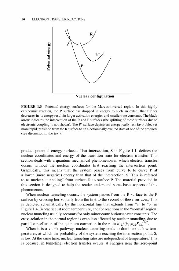
The reason for this can be understood by reference to Figure 1.1. The plots in

Figure 1.1 show the locations of theR andP surfaces in the normal region. To reach the

inverted region,DG�0 must becomemore negative. This corresponds to lowering the P

surface relative to the R surface in Figure 1.1. As this proceeds, the free energy barrier

DGz decreases until it becomes zero atDG�0 ¼�l. At this point, the intersection of theR and P surfaces occurs at the minimum of the R curve, and the reaction has no

activation barrier. Further decrease inDG�0 then raises the energy at which the R and P

surfaces intersect. This corresponds to an increase in the activation barrier, DGz, anda decrease in rate. This case, that is, the inverted region, is shown in Figure 1.3, which

depicts the relative locations of the reactant and product energy surfaces in the

inverted region.

Indirect evidence for the inverted region was first provided by observations that

some highly exothermic electron transfer reactions resulted in chemiluminescence,

an indication that electronically excited products had been formed (surface P in

Figure 1.3).When the ground electronic state potential energy surface of the products,

P, intersects the R surface at a point high in energy on the R surface (intersection of

curves R and P in the inverted region; Figure 1.3), the reaction is slow. In this case, less

thermodynamically favorable electron transfer to a product excited state (P surface)can occur more rapidly than electron transfer to the ground electronic state of the

products (P surface). Electron transfer to a P state, and chemiluminescence asso-

ciated with a subsequent loss of energy to give the ground electronic state, was

observed by Bard and coworkers.24 Direct experimental confirmation of the inverted

region (electron transfer from the R to P surfaces in Figure 1.3) was provided a few

years later.25,26

1.2.8 Nuclear Tunneling

The Marcus equation (and useful relationships derived from it) is a special case

characterized by adiabatic electron transfer at the intersection of the reactant and

I II

–ΔGº′

ln k

III

FIGURE 1.2 Plot of ln k versus �DG�0. Region I is the normal region, region III is the

inverted region, and at point II (�DG�0 ¼ l) ln k reaches a maximum.


product potential energy surfaces. That intersection, S in Figure 1.1, defines the

nuclear coordinates and energy of the transition state for electron transfer. This

section deals with a quantum mechanical phenomenon in which electron transfer

occurs without the nuclear coordinates first reaching the intersection point.

Graphically, this means that the system passes from curve R to curve P at

a lower (more negative) energy than that of the intersection, S. This is referred

to as nuclear “tunneling” from surface R to surface P. The material provided in

this section is designed to help the reader understand some basic aspects of this

phenomenon.

When nuclear tunneling occurs, the system passes from the R surface to the P

surface by crossing horizontally from the first to the second of these surfaces. This

is depicted schematically by the horizontal line that extends from “a” to “b” in

Figure 1.4. In practice, at room temperature, and for reactions in the “normal” region,

nuclear tunneling usually accounts for onlyminor contributions to rate constants. The

cross-relation in the normal region is even less affected by nuclear tunneling, due to

partial cancellation of the quantum correction in the ratio k12=ðk11k22K12Þ1=2.When it is a viable pathway, nuclear tunneling tends to dominate at low tem-

peratures, at which the probability of the system reaching the intersection point, S,

is low. At the same time, nuclear tunneling rates are independent of temperature. This

is because, in tunneling, electron transfer occurs at energies near the zero-point

FIGURE 1.3 Potential energy surfaces for the Marcus inverted region. In this highly

exothermic reaction, the P surface has dropped in energy to such an extent that further

decreases in its energy result in larger activation energies and smaller rate constants. The black

arrow indicates the intersection of the R and P surfaces (the splitting of these surfaces due to

electronic coupling is not shown). The P surface depicts an energetically less favorable, yet

more rapid transition from the R surface to an electronically excited state of one of the products

(see discussion in the text).


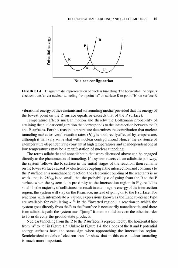
vibrational energy of the reactants and surroundingmedia (provided that the energy of

the lowest point on the R surface equals or exceeds that of the P surface).

Temperature affects nuclear motion and thereby the Boltzmann probability of

attaining the nuclear configuration that corresponds to the intersection between the R

and P surfaces. For this reason, temperature determines the contribution that nuclear

tunnelingmakes to overall reaction rates. (HAB is not directly affected by temperature,

although it will vary somewhat with nuclear configuration.) Hence, the existence of

a temperature-dependent rate constant at high temperatures and an independent one at

low temperatures may be a manifestation of nuclear tunneling.

The terms adiabatic and nonadiabatic that were discussed above can be engaged

directly to the phenomenon of tunneling. If a system reacts via an adiabatic pathway,

the system follows the R surface in the initial stages of the reaction, then remains

on the lower surface caused by electronic coupling at the intersection, and continues to

the P surface. In a nonadiabatic reaction, the electronic coupling of the reactants is so

weak, that is, 2HAB is so small, that the probability k of going from the R to the P

surface when the system is in proximity to the intersection region in Figure 1.1 is

small. In themajority of collisions that result in attaining the energy of the intersection

region, the system will stay on the R surface, instead of going on to the P surface. For

reactions with intermediate k values, expressions known as the Landau–Zener type

are available for calculating k.13 In the “inverted region,” a reaction in which the

system goes directly from the R to the P surface is necessarily nonadiabatic, and there

is no adiabatic path: the systemmust “jump” from one solid curve to the other in order

to form directly the ground-state products.

Nuclear tunneling from the R to the P surfaces is represented by the horizontal line

from “a” to “b” in Figure 1.5. Unlike in Figure 1.4, the slopes of the R and P potential

energy surfaces have the same sign when approaching the intersection region.

Semiclassical models of electron transfer show that in this case nuclear tunneling

is much more important.

FIGURE 1.4 Diagrammatic representation of nuclear tunneling. The horizontal line depicts

electron transfer via nuclear tunneling from point “a” on surface R to point “b” on surface P.


1.2.9 Reactions of Charged Species and the Importance of Electrolyte Theory

1.2.9.1 Background and Useful Models The Marcus equation is an extension of

earlier models from collision rate theory. As such, compliance with collision rate

models is a prerequisite to defensible use of the Marcus equation. This is particularly

important for reactions of charged species, and therefore, for reactions of many

inorganic complexes. In these cases, the key question is whether electron transfer rate

constants vary with ionic strength as dictated by electrolyte theory, on which the

collision ratemodels are based.When they do not, differences between calculated and

experimental values can differ by many orders of magnitude.

The theory of electrolyte behavior in solution is indeed complex, and has been

debated since 1923, when Debye and H€uckel27,28 described the behavior of electro-

lyte solutions at the limit of very low concentration. Subsequently, intense discussions

in the literature lasted into the 1980s, by which time a number of quite complex

approaches had been promulgated. The latter do give excellent fits up to large ionic

strength values, but are generally not used by most kineticists.

The effects of electrolyte concentrations on the rate constants depend on the nature

of the interaction between the reacting species. If the reacting species repel

one another, rate constants will increase with ionic strength. This is because the

electrolyte ions attenuate electrostatic repulsion between the reacting ions. If the

reactants have opposite charges, and attract one another, electrolyte ions will

attenuate this attraction, resulting in smaller rate constants.

One convenient option is to use the Debye–H€uckel equation, also referred to as theDavies equation.29

FIGURE1.5 Diagrammatic representation of nuclear tunneling from “a” to “b” in the highly

exothermic (inverted) reaction.


log k ¼ log k0 þ2z1z2a

ffiffiffiffim

p1þ br

ffiffiffiffim

p ð1:27Þ

In Equation 1.27, a and b are the Debye–H€uckel constants, equal to 0.509 and

0.329, respectively, at 25�C in aqueous solutions. k0 is the rate constant for the

reaction at infinite dilution (m¼ 0M). In this form, a is dimensionless and b has units

of A� 1/2/mol1/2.

One fundamental problem is that kineticists almost always deal with solutions of

mixed electrolytes. In such cases, the Davies equation is not rigorously correct (based

onfirst principles from thermodynamics). In addition, someworkers argue that setting

the parameter r equal to the internuclear distance between reacting species is not

justified, and that successful results obtained by doing so should be viewed as

fortuitous.30 Nonetheless, as is demonstrated later in this chapter, it can give excellent

results in some cases.31–34

Alternatively, one may use the Guggenheim equation (Equation 1.28), which is

rigorously correct for solutions of mixed electrolytes. In this equation, the specific

interaction parameters aremoved from the denominator to a second term, inwhich b is

an adjustable parameter.


ffiffiffiffim

p1þ ffiffiffiffi

mp þ bm ð1:28Þ

If one ignores the second term in Equation 1.28, one obtains the “truncated”

Guggenheim equation (Equation 1.29), which is identical to the Davies equation, but

with br equal to unity. The reader should be aware that many authors refer to

Equation 1.29 as the Guggenheim equation.


ffiffiffiffim

p1þ ffiffiffiffi

mp ð1:29Þ

Alternatively, one can use more elaborate models.35 These can yield fine fits to

extraordinarily high ionic strengths, but they do not generally provide much addi-

tional insight.

In practice, the most common approach36 is to use the truncated Guggenheim

equation (Equation 1.29) and ionic strength no greater than 0.1M. This is also

the method espoused by Espenson.37 If this fails, the Guggenheim equation

(Equation 1.28) is sometimes used. This hasmore adjustable parameters, and therefore

is more likely to produce a linear fit. However, the slopes of the lines obtained often

deviate from theoretical values, defined as a function of the charge product, z1z2, of the

reacting species. Nonetheless, if a good linear fit is obtained (even though the slope is

not correct), this might still be used as an argument against the presence of significant

ion pairing or othermedium effects. A good example of this is provided in an article by

Brown and Sutin,38 who fitted the same data set to a number of models before finally

observing a linear relationship between rate constants and ionic strength.


1.2.9.2 Graphical Demonstration of the Truncated Guggenheim Equation In

Figure 1.6, the truncated Guggenheim equation (Equation 1.29) was used to calculate

rate constants as a function of ionic strength. Then, log k values were plotted as

a function of ionic strength. This reveals the effects of ionic strength on rate constants

that one might observe experimentally. The curves shown are for reactions with

charge products of z1z2¼�2, �1, 0, 1, and 2. Charge products of 2 and 1 indicate

repulsion between like-charged reactants and those of �1 and �2 indicate attraction

between oppositely charged reactants.

In Figure 1.7, the same rate constants and ionic strengths shown in Figure 1.6 are

now plotted according to the truncated Guggenheim equation (Equation 1.29). The

horizontal line corresponds to z1z2¼ 0. The slopes of the lines are equal to 2z1z2a andhave values of �2.036, �1.018, 0, 1.018, and 2.036, respectively, for z1z2 values of

�2, �1, 0, 1, and 2.

As discussed above, verification that a reaction that involves charged species

satisfies the requirements of electrolyte theory is a necessary prerequisite to use of the

Marcus model. For this, a plot of log k versusffiffiffiffim

p=ð1þ ffiffiffiffi

mp Þ (truncated Guggenheim

equation) should be linear with a slope of 2z1z2a, as shown in Figure 1.7. Deviationsfrom linearity, or, to a lesser extent, slopes that give incorrect charge products, z1z2,

are indications that the system does not obey this model. When this occurs, other

models can be tried. If these fail, ion pairing, other specific medium effects, cation

catalysis, or other reaction mechanisms are likely involved.21 In these cases, the

reaction is not a defensible candidate for evaluation by the Marcus model for outer-

sphere electron transfer.

Finally, readers should be aware of a comment by Duncan A. MacInnes (in

193939) that “There is no detail of the derivation of the equations of the

FIGURE 1.6 Theoretical plots of log k versus ionic strength m for charge products z1z2¼ 2,

1, 0, �1, and �2. The zero ionic strength rate constant k0 is set equal to 100M�1 s�1 and m is

varied from 0.001 to 1M.


Debye–H€uckel theory that has not been criticized.” From this perspective, electro-

lyte models are simply the best tools available to assess whether the dependence of

electron transfer rate constants on ionic strength is sufficiently well behaved to

justify use of the Marcus model. For this, and despite their shortcomings, they are

indispensable.

1.3 GUIDE TO USE OF THE MARCUS MODEL

This section is designed to fill the gap between the familiar “formulas” presented

above and the assumptions and definitions of terms and physical constants needed to

apply them. Values for all physical constants and needed conversion factors are

provided, and dimensional analyses are included to show how the final results and

their units are obtained. This close focus on the details and units of the equations

themselves is followed by worked examples from the chemical literature. The goal is

to provide nearly everything the interested reader may need to evaluate his or her own

data, with reasonable confidence that he or she is doing so correctly.

1.3.1 Compliance with Models for Collision Rates Between Charged Species

In this section, applications of the Davies and truncated Guggenheim equations are

demonstrated through worked examples from the literature.

1.3.1.1 The Davies Equation The Davies equation (introduced earlier in this

chapter and reproduced here for convenience in Equation 1.30) is one of several

closely related models, derived from electrolyte theory, that describe the functional

FIGURE 1.7 Plots of log k versusffiffiffiffim

p=ð1þ ffiffiffiffi

mp Þ for charge products z1z2¼ 2, 1, 0,�1, and

�2. k0 is taken as 100M�1 s�1 and the ionic strength m is varied from 0.001 to 1M.

GUIDE TO USE OF THE MARCUS MODEL 19

dependence of rate constants on ionic strength.

log k ¼ log k0 þ 2az1z2 m1=2=ð1þ brm1=2Þ ð1:30Þ

In Equation 1.30, z1 and z2 are the (integer) charges of the reacting ions and r is the

hard sphere collision distance (internuclear distance). The latter term, r, is approxi-

mated as the sum of the radii of the reacting ions, r1 þ r2.18 The term m is the total

ionic strength. It is defined as m ¼ 12

Pniz

2i for electrolyte solutions that contain

molar concentrations, ni, of species i of charge z. The constant a is dimensionless

and equal to 0.509, and for r in units of cm, b¼ 3.29� 107 cm1/2/mol1/2. Finally, log k

in Equation 1.30 refers to log10 k, rather than to the natural logarithm, ln k. This

deserves mention because in many published reports, log k is (inappropriately) used

to refer to ln k.

Typically, log k (i.e., log10 k) is plotted (y-axis) as a function of m1/2/(1 þ brm1/2)

(x-axis). If the result is a straight line, its slope should be equal to a simple function of

the charge product, that is, 2z1z2a, and its y-intercept gives log k0, the log of the rateconstant at the zero ionic strength limit. The constant k0 is the ionic strength-

independent value of the rate constant and can be treated as a fundamental parameter

of an electron transfer reaction.

1.3.1.2 Dimensional Analysis The constant b in Equation 1.31 is the “reciprocal

Debye radius.”11,16Dimensional analysis of this term is instructive because it involves

a number of often needed constants and occurs frequently in a variety of contexts.

b � 8pNe2=1000DskT ð1:31Þ

The following values, constants, and conversion factors apply:

Conditions: 298K (25�C) in water

N¼Avogadro’s number (6.022� 1023mol�1)

e¼ electron charge (4.803� 10�10 electrostatic units (esu) or StatC)

Ds¼ static dielectric constant (78.4) (water at 298K)

k¼Boltzmann constant (1.3807� 10�16 erg/K)

1 StatC2=cm ¼ 1 erg ð1:32Þ

Evaluation of b is as follows:

b ¼ 8pNe2

1000Ds kT

� �1=2

ð1:33Þ

b ¼ 8pð6:022� 1023 mol�1Þð4:803� 10�10 StatCÞ21000ð78:4Þð1:3807� 10�16erg=KÞ298K

!1=2

ð1:34Þ


b ¼ 8pð6:022� 1023 mol�1Þð4:803� 10�10 StatCÞ21000ð78:4Þð1:3807� 10�16erg=KÞ298K

ðerg cmÞStatC2

!1=2

ð1:35Þ

b ¼ 3:29� 107 cm1=2=mol1=2 ð1:36Þ

In theDavies equation (Equation 1.30),b ismultiplied by r. If this distance is in cm,

one obtains

b � cm ¼ ð3:29� 107 cm1=2=mol1=2Þcm ð1:37Þ

which is equivalent to Equation 1.38.

b � cm ¼ 3:29� 107cm3

mol

� �1=2

ð1:38Þ

The units in Equation 1.38 can be viewed as (vol/mol)1/2 and are cancelled (i.e.,

reduced to unity) when multiplied by the units of m1/2 (mol/vol)1/2 in the Davies

equation (Equation 1.30).

Note here that the denominator in Equation 1.33 (definition of b) is multiplied by

a factor of 1000. This is needed to “scale up” from cm3 to L, so that, for r in cm and min mol/L, the units associated with the product brm exactly cancel one another.

Similarly, for r in units of A�and m in units of mol/L, b ¼ 0:329 A

� 1=2=mol1=2.

In published articles, b is often presented as dimensionless (e.g., as 0.329), or with

units of cm�1 or A� �1. The units of cm�1 are obtained if the correction factor of 1000 in

the denominator of Equation 1.33 is assigned units of cm3. Once the final units are in

cm�1, these can be converted to A� �1. These options can be disconcerting to those new

to the use of these models. For practical purposes, however, one only needs to know

that, form in units of molarity (M), b¼ 0.329 for r in units of A�and 3.29� 107 for r in

units of cm.

1.3.1.3 Literature Example: Reaction Between a-PW12O404� and a-PW12O40

3�

In a detailed investigation of electron self-exchange between Keggin heteropoly-

tungstate anions in water, Kozik and Baker used line broadening of 31P NMR signals

to determine the rates of electron exchange between a-PW12O403� and one-electron

reduced a-PW12O404� (Figure 1.8) and between a-PW12O40

4� and the two-electron

reduced anion a-PW12O40.5�31,40 TheW ions in the parent anion a-PW12O40

3� are in

their highest þ 6 oxidation state (d0 electron configuration).

Structurally, a-PW12O403�, which is 1.12 nm in diameter,41 may be viewed as a

tetrahedral phosphate anion, PVO43�, encapsulated within a neutral, also tetrahedral,

a-WVI12O36

0 shell (“clathrate” model42–44). According to this model, the PVO43�

anion in the one-electron reduced anion, a-PW12O404�, is located at the center of

a negatively charged W12O36� shell,45 which contains a single d (valence) electron.

Moreover, the single valence electron is not localized at any single W atom, but is


rapidly exchanged between all 12 chemically equivalent W centers. The rate of

intramolecular exchange at 6K is �108 s�1 and considerably more rapid46,47 than

most electron transfer reactions carried out at near-ambient temperatures between the

reduced anion, a-PW12O404�, and electron acceptors.

Kozik and Baker combined the acid forms of the two anions, a-H3PW12O40 and

a-H4PW12O40 (1.0mM each), in water using a range of ionic strengths (m) from0.026 to 0.616M.31 Ionic strength values were adjusted by addition of HCl and NaCl

(pH values ranged from 0.98 to 1.8). Under these conditions, the anions are present in

their fully deprotonated, “free anion” forms, a-PW12O403� and a-PW12O40

4�.Observed rate constants, kobs, were fitted to the Davies equation (Equation 1.30).

An internuclear distance of r¼ 11.2A�, or twice the ionic radius of the Keggin anions,

was used. At 25�C inwater, a¼ 0.509 (dimensionless) and b¼ 3.29� 107 cm/mol1/2.

FIGURE 1.8 Electron self-exchange between a-PW12O404� and a-PW12O40

3�. The

a-Keggin anions are shown in coordination polyhedron notation. Each anion is 1.12 nm in

diameter and possesses tetrahedral (Td) symmetry. In each anion, the 12Waddendum atoms are

at the center of WO6 polyhedra that each have C4v symmetry. At the center of each cluster

(shaded) is a tetrahedral phosphate oxoanion, PO43�.


For the units to “work out,” r must be converted to 1.12� 10�7 cm. Using

Equation 1.30, log kwas plotted as a function ofm1/2/(1 þ brm1/2). A linear relation-

ship was observed (R2¼ 0.998), whose slope (equal to 2az1z2) gave a charge productof z1z2¼ 14.3 (Figure 1.9). The theoretical charge product is 12. Linearity and

comparison to the theoretical charge product are both important considerations in

evaluating whether an electron transfer reaction between charged species obeys

electrolyte theory to an extent sufficient for proceeding with use of the data in the

Marcus model. In the present case, few would argue that the system fails to comply

with electrolyte theory.

The linearity and close-to-theoretical slope in Figure 1.9 was surprising because

Equation 1.30 was derived for univalent ions at low ionic strengths (up to 0.01M).

Agreement at much higher ionic strengths (greater than 0.5M) was attributed to the

fact that POM anions, “owing to the very pronounced inward polarization of their

exterior oxygen atoms, have extremely low solvation energies and very low van der

Waals attractions for one another.”48

In many published examples of careful work, some models fail, while others

(including those with empirical corrections) give better fits. In those cases, some

judgment is required to assess whether the Marcus model might be used. The most

often encountered reasons for failure to comply with these models are the presence of

alternative mechanistic pathways and significant ion association between electrolyte

ions and the charged species involved in the electron transfer reaction. Ion association

is discussed in more detail at the end of this chapter.

1.3.2 Self-Exchange Rate Expression

For self-exchange reactions such as that in Figure 1.8, Equation 1.18 applies. This is

obtained by setting the free energy terms in Equation 1.12 equal to zero. Inmost cases,

thework termW(r) can be calculated. This is the energy required to bring the reactants

from effectively infinite separation towithin collision distance r, approximated as the

FIGURE 1.9 Plot of log k as a function of m1/2/(1 þ brm1/2) (from the Davies equation,

Equation 1.30). The slope of the line (equal to 2az1z2) gives a charge product z1z2 of 14.3.


sum of the radii of the reacting ions, r1 þ r2. The reorganization energy l is more

difficult to calculate. This is because it requires detailed knowledge of all the changes

in bond lengths and angles required to reach the transition state for electron transfer

(see Equation 1.9) and this information is usually not available. In practice, therefore,

self-exchange reactions are most commonly carried out as a means for determining

the reorganization energies. This fundamental parameter of the self-exchange reac-

tion can then be used to determine the inherent reorganization barriers associated

with other electron transfer reactions (cross-reactions) of interest. In this sense, the

species involved in the self-exchange reaction can be deployed as physicochemical

“probes.”17,32,33

The work term W(r), Equation 1.39, is as shown in Equation 1.4, but with

the subscript on the collision distance r modified to indicate a self-exchange

reaction.

WðrÞ ¼ z1z2e2

Dr11expð�wr11Þ ð1:39Þ

Equation 1.39 is commonly written in a more convenient form (Equation 1.40).

WðrÞ ¼ z1z2e2

Dr11ð1þ brm1=2Þ ð1:40Þ

The dimensional analysis provided in Equations 1.33–1.38 applies here as well,

and the electron charge, e, needed here is equal to 4.803� 10�10 StatC. To use

Equation 1.40, a conversion factor must be added, as shown in Equation 1.41.

WðrÞ ¼ z1z2ð4:803� 10�10 StatCÞ2Dr11ð1þ brm1=2Þ 1:439� 1013

kcal=mol

StatC2=cm

� �ð1:41Þ

To evaluate this expression, r is given in units of cm. Because z1, z2, and the static

dielectric constant D are dimensionless, and (as noted above) the units of the term

brm1=2exactly cancel one another, the units in Equation 1.41 reduce to kcal/mol.

A dramatic example of the effect of charge and W(r) on rate constants involves

self-exchange between a-AlW12O405� and the one-electron reduced anion

a-AlW12O406�. At an ionic strength, m, of 175mM, the rate constant for this reaction

is 3.34� 102M�1 s�1. By comparison, the rate constant for self-exchange between

a-PW12O403� and the 1e�-reduced anion a-PW12O40

4� at m¼ 175mM is 2.28� 107

M�1 s�1. Work terms and reorganization energies for the two reactions at this ionic

strength areW(r)¼ 4.46 and 1.78M�1 s�1 for charge products, respectively, of 30 and

12. (Also responsible in part for the difference in self-exchange rate constants is the

decrease in reorganization energies from 8.8 to 6.1 kcal/mol between the slower and

faster reactions.)

By taking the natural logarithm of each side of Equation 1.18, one obtains

Equation 1.42 (reproduced here from Section 1.2). The subscript on k is a pair of


1’s, used to indicate that this rate constant is for a self-exchange reaction.

ln k11 ¼ ln Z�WðrÞRT

� l4RT

ð1:42Þ

Hence, by measuring the rate of electron self-exchange, one can readily use the

Marcus model to calculate the reorganization energy l. To evaluate this, a collision

frequencyofZ¼ 1011M�1 s�1 isgenerallyused, and the temperature isgiven inKelvin.

1.3.2.1 Literature Examples: RuIII(NH3)63þ þ RuII(NH3)6

2þ and O2 þ O2�

A well-known self-exchange reaction is that between RuIII(NH3)63þ and

RuII(NH3)62þ .38,49 At 25�C and m¼ 0.1M, the experimentally determined self-

exchange rate constant k11 is 4� 103M�1 s�1.

ForD¼ 78.4, the effective radius of the Ru complexes equal to 3.4� 10�8 cm (i.e.,

r¼ 6.8� 10�8 cm), and the other constants defined as shown above,W(r) is calculated

as shown in Equation 1.43.

WðrÞ ¼ 3 � 2ð4:803� 10�10 StatCÞ278:4 � ð6:8� 10�8 cmÞð1þ3:29� 107 cm1=2=mol1=2ð6:8� 10�8 cmÞð0:1mol=LÞ1=2Þ

� 1:439� 1013kcal=mol

StatC2=cm

� �¼ 2:19 kcal=mol

ð1:43Þ

The ionic strengthm in units ofmol/L is equivalent to units ofmmol/cm3. Note that

b has units of cm1/2/mol1/2, such that the units of the product brm cancel one another

due to the factor of 1000 in the denominator of b itself (i.e., as defined in

Equation 1.33).

By solving Equation 1.42 for l, one obtains

l ¼ 4ðRT ln Z�RT ln k11�WðrÞÞ ð1:44Þ

Substitution of Z¼ 1011,D¼ 78.4,R¼ 1.987� 10�3 kcal/mol, k11¼ 4� 103M�1

s�1, and W(r)¼ 2.19 kcal/mol into Equation 1.44 gives l¼ 31.6 kcal/mol. In this

reaction, the work required to bring the charged reactants into close proximity is

considerably smaller than the reorganization energy needed to reach the transition

state for electron transfer.

In the above example, the reorganization energy l is the total reorganization

energy and includes both inner-sphere and outer-sphere components, lin and lout,discussed earlier in this chapter. Once the total reorganization energy, ltotal, is known,lin and lout can be calculated using Equation 1.45.

ltotal ¼ lin þ lout ð1:45Þ

As noted earlier, information needed to calculate lin (Equation 1.9) is usually notreadily available. However, lout is easily calculated using Equation 1.10. For


self-exchange reactions, r1¼ r2 and r12¼ 2 r1, and for a one-electron process, De¼ e.

Thus, Equation 1.10 reduces to Equation 1.46.

lout ¼ e21

r1

� �1

h2� 1

Ds

� �ð1:46Þ

Here, h andDs are the refractive index and static dielectric constant of the solvent. In

water at 298K, h¼ 1.33 and Ds¼ 78.4.

An important application of Equations 1.45 and 1.46 involves analysis of electron

exchange between dioxygen (O2) and the superoxide radical anion (O2�) in water.

Lind andMer�enyi determined the rate constant for this reaction by reacting 32O2 with

isotopically labeled O2� (Equation 1.47).50 The labeled superoxide anion was

generated by g-irradiation of 36O2.

32O2 þ 36O�2 ! 32O�

2 þ 36O2 ð1:47Þ

They obtained a rate constant of 450� 150M�1 s�1. Because the charge product

for this reaction, z1z2, is equal to zero (the charge onO2 is zero),W(r) in Equation 1.44

is equal to zero, and that equation reduces to

ltotal ¼ 4RT lnZ

k11

� �ð1:48Þ

The experimentally determined rate constant gave ltotal¼ 45.5 kcal/mol. In this

case, it was possible to estimate lin computationally (which involves lengthening of

the O–O bond), and then use Equation 1.45 to determine lout. They estimated that

lin¼ 15.9 kcal/mol, which left 29.6 kcal/mol for lout. Next, they used Equation 1.46

to calculate the “effective” radius of O2 (i.e., r1/2) and obtained a value of 3A�.

More recent work suggests that this seemingly large value might reflect orienta-

tional restrictions imposed on collisions between the nonspherical reactants, O2

and O2�.51

1.3.3 The Marcus Cross-Relation

Rate constants for outer-sphere electron transfer reactions that involve net changes

in Gibbs free energy can be calculated using the Marcus cross-relation

(Equations 1.24–1.26). It is referred to as a “cross-relation” because it is derived

from expressions for two different self-exchange reactions.

1.3.3.1 Derivation of the Marcus Cross-Relation The cross-relation is derived

algebraically by first assuming that the reorganization energy for the “cross” reaction

is the average of the reorganization energies associated with the two self-exchange

reactions involved. To clarify this, consider the two self-exchange reactions in

Equations 1.49 and 1.50. These reactions are, respectively, assigned rate constants


of k11 and k22, which are associated with reorganization energies l11 and l22. Thereorganization energies are inherent properties of these exchanging pairs.

Ared þA*ox >Aox þA*

red ð1:49Þ

Bred þB*ox >Box þB*

red ð1:50Þ

Associated with these self-exchange reactions are two “cross” reactions

(Equations 1.51 and 1.52). Unlike the self-exchange reactions, the cross-reactions

are functions of (almost always) nonzero Gibbs free energies DG�12 and DG�

21 (the

subscripts indicate a “cross” reaction and are arbitrarily assigned here to one reaction

and its reverse). Once the rate constants of the self-exchange reactions, and the Gibbs

free energy for the cross-reactions, are known, the MCR can be used to predict the

rate constants, k12 or k21, for each cross-reaction.

Ared þBox >Aox þBred; rate constant ¼ k12 ð1:51Þ

Aox þBred >Ared þBox; rate constant ¼ k21 ð1:52Þ

To derive the MCR, it is necessary to assume that the reorganization energies for

the reactions shown in Equations 1.51 and 1.52 are both equal to the mean of l11 andl22 (Equation 1.53).

l12 ¼ 1

2ðl11 þ l22Þ ð1:53Þ

Next, Equation 1.53 is algebraically combined with equations that describe the

dependence of k11 and k22 on l11 and l22 (Equations 1.54 and 1.55) and the

dependence of k12 on l12 and DG�012 (Equation 1.56).

ln k11 ¼ w11 þ l114

ð1:54Þ

ln k22 ¼ w22 þ l224

ð1:55Þ

ln k12 ¼ WðrÞ12 þl124

1þ DG�012

l12

� �2

ð1:56Þ

The Gibbs energy term in Equation 1.56 is not the standard Gibbs free energy,

DG�12, for the cross-reaction in Equation 1.51. Rather, it is the “corrected” Gibbs free

energy, DG�012: the difference in energy between the successor and precursor com-

plexes in Scheme 1.2.

The corrected Gibbs free energy is related toDG�12 by the relation in Equation 1.57,

where wij are the Coulombic energies of formation of individual (often short-lived)


association complexes. The wij terms are retained in the MCR and will be further

clarified below through a worked example.

DG�012 ¼ DG

�12 þw21�w12 ð1:57Þ

Substituting Equation 1.58 into Equation 1.57 gives Equation 1.59.

DG�12 ¼ �RT ln K12 ð1:58Þ

DG�012 ¼ �RT ln K12 þw21�w12 ð1:59Þ

Using Equations 1.53–1.56 and 1.59, approximately 30 algebraic steps lead

to Equations 1.60–1.62 (reproduced here for convenience from Section 1.2). (The

equilibrium constant K12, rather than a Gibbs free energy term, appears in Equa-

tion 1.60, and it is incorporated by substitution of Equation 1.59 into Equation 1.56.)

k12 ¼ ðk11k22K12 f12Þ1=2 C12 ð1:60Þ

where

ln f12 ¼ 1

4

ðlnK12 þðw12�w21Þ=RTÞ2lnðk11k22=Z2Þþ ðw11�w22Þ=RT ð1:61Þ

and

C12 ¼ exp½�ðw12 þw21�w11�w22=2RTÞ� ð1:62Þ

The use of this relation requires that Equation 1.53 be valid. Equation 1.53, in turn,

is a good approximation for the reorganization energy of the cross-reaction (either

SCHEME 1.2


Equation 1.51 or 1.52) only when the reacting species are spherical in shape and

identical to one another in size. One of the model’s strengths is that reasonable results

(within�1 order ofmagnitude between calculated and experimental values) can often

be obtained for reactions between electron donors and acceptors that do notmeet these

criteria. This is fortunate because few reactions do.

1.3.3.2 Literature Examples: a-AlW12O406� þ a-PW12O40

4� and a-PW12O40

4� þ O2 The MCR is used here to calculate the rate constant, k12, for

electron transfer from to a-AlW12O406� (one-electron reduced) to a-PW12O40

4�

(one-electron reduced) to give a-PW12O405� (the two-electron reduced ion)

(Equation 1.63).32

a-AlW12O6�

40 þ a-PW12O4�

40 ! a-AlW12O5�

40 þ PW12O5�

40 ð1:63Þ

The MCR will be used below to calculate the rate constant, k12(calc), for this

reaction and to compare that value with the experimentally determined rate constant,

k12(exp). For this, k12(exp) was determined as shown immediately below. In this

example, “zero ionic strength” rate constants are used. These are obtained from plots

of rate versus functions of ionic strength derived from electrolyte theory. If these plots

give straight lines with slopes near theoretical (i.e., slopes that give the actual charge

product, z1z2), then extrapolation to zero ionic strength is defensible.Aswill be shown

in a subsequent example, however, the use of zero ionic strength rate constants is not

required for use of the MCR.

To determine k12(exp), solutions of a-AlW12O406� and a-PW12O40

4� (the latter in

largemolar excess)weremixed in a stopped-flowapparatus.Thechange in absorbance

with time (determined by UV-Vis spectroscopy) was exponential, and pseudo-first-

order rate constants, kobs, were determined from each absorbance versus time curve

(to�100%completion of reaction). Plots of these rate constants as a function of initial

a-PW12O404� concentration at three ionic strength values gave three straight lines

(Figure 1.10). The slopes of these lines are the bimolecular rate constants, k12, for the

reaction at each of the three ionic strength values used. The range of experimentally

useful ionic strength values was limited by practical considerations, but adequate.

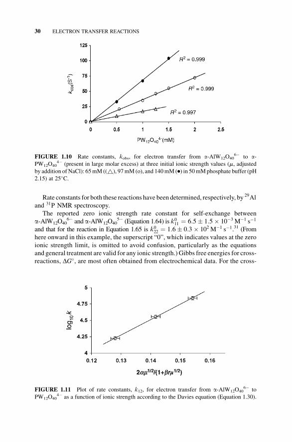
The three bimolecular rate constants, k12, from Figure 1.10, were plotted as

a function of ionic strength using the extended Davies equation (Figure 1.11). The

slope (R2¼ 0.9997) gave a charge product (z1z2) of 23� 1, within experimental

uncertainty of the theoretical value of 24. Extrapolation to zero ionic strength gave

k022ðexpÞ ¼ 17� 2M�1 s�1 (the superscript “0” is used to indicate that this value

refers to zero ionic strength).

TheMCRwill now be used to obtain k12(calc) from the two relevant self-exchange

reactions in Equations 1.64 and 1.65:

*a-AlW12O6�

40 þ a-AlW12O5�

40 ! *a-AlW12O5�

40 þ a-AlW12O6�

40 ð1:64Þ

*a-PW12O5�

40 þ a-PW12O4�

40 ! *a-PW12O4�

40 þ a-PW12O5�

40 ð1:65Þ


Rate constants for both these reactions have been determined, respectively, by 29Al

and 31P NMR spectroscopy.

The reported zero ionic strength rate constant for self-exchange between

a-AlW12O406� and a-AlW12O40

5� (Equation 1.64) is k011 ¼ 6:5� 1:5� 10�3 M�1 s�1

and that for the reaction in Equation 1.65 is k022 ¼ 1:6� 0:3� 102 M�1 s�1.31 (From

here onward in this example, the superscript “0”, which indicates values at the zero

ionic strength limit, is omitted to avoid confusion, particularly as the equations

and general treatment are valid for any ionic strength.) Gibbs free energies for cross-

reactions, DG�, are most often obtained from electrochemical data. For the cross-

FIGURE 1.10 Rate constants, kobs, for electron transfer from a-AlW12O406� to a-

PW12O404� (present in large molar excess) at three initial ionic strength values (m, adjusted

by addition ofNaCl): 65mM ((~), 97mM (o), and 140mM (.) in 50mMphosphate buffer (pH

2.15) at 25�C.

FIGURE 1.11 Plot of rate constants, k12, for electron transfer from a-AlW12O406� to

PW12O404� as a function of ionic strength according to the Davies equation (Equation 1.30).


relation, the reduction potentials of the individual self-exchange reactions are used

to calculate the equilibrium constant for the cross-reaction,K12. Reported reduction

potentials (relative to the normal hydrogen electrode, NHE) are �130� 5 and

�10� 5mV, respectively, for the self-exchanging redox couples a-AlW12O405�/a-

AlW12O406� and a-PW12O40

5�/a-PW12O404�. The equilibrium constant is calcu-

lated by rearranging Equation 1.58 to give Equation 1.66.

K12 ¼ exp �DG�12

RT

� �ð1:66Þ

DG�12 is calculated from electrochemical data using the definition of the standard

potential (Equation 1.67), where n is the charge number of the reaction, that is, the

number of electrons involved, and F is the Faraday constant. In convenient units,

F¼ 23.06 kcal/(mol V).

DG�12 ¼ �nFE

� ð1:67Þ

Thus, standard potential for the reaction in Equation 1.63 is equal to the reduction

potential of the species reduced in the reaction, minus the potential of the electron

donor, that is, �10� (�130)mV, which is equal to þ 0.12V. Hence,

DG�12 ¼ 2:77 kcal=mol (from Equation 1.58). By using Equation 1.66 with R¼ 1.987

� 10�3 kcal/(mol K) and T¼ 298K, K12¼ 107.

We now have experimentally determined values for k11, k22, andK12. The next step

in applying the MCR is to evaluate the terms ln f12 and C12. In reactions between

species whose charges are small or similar to one another, it is often possible to obtain

a reasonably good result by setting both f12 and C12 equal to 1, such that the MCR

reduces to Equation 1.68.

k12 ¼ ðk11k22K12Þ1=2 ð1:68Þ

Using Equation 1.68, k012ðcalcÞ ¼ ½ð6:5� 10�3M�1s�1Þð1:6� 102 M�1 s�1Þð107Þ�1=2 ¼ 10:5M�1 s�1. For calculations of this type, the agreement between this

value and the experimental one (17� 2M�1 s�1) is quite good.

This result can be improved upon by including ln f12 andC12. For this, thewij terms

in Equations 1.61 and 1.62 must be evaluated, and the subscripts on the wij terms

correctly interpreted. Consider the cross-reaction as written in Equation 1.69:

a-AlW12O6�

40 þ a-PW12O4�

40 ! a-AlW12O5�

40 þ PW12O5�

40

1red 2ox 1ox 2redð1:69Þ

The numbers 1 or 2 under each of the four species refer to the two self-exchange

reactions (Equations 1.64 and 1.65), associated, respectively, with the rate constants

k11 and k22. For the first self-exchange reaction (involving a-AlW12O406� and k11),

the electron donor is 1red and its corresponding oxidized form is 1ox. For the


self-exchange reaction involving a-PW12O404� and k22 (Equation 1.65), the electron

acceptor is 2ox and the corresponding product of electron transfer is 2red.

The wij terms are identical to W(r) as defined in Equations 1.40 and 1.41. To

evaluate them, it is necessary to know the charge products, zizj, and distances of

closest approach, rij. These can be obtained using Table 1.1.

An exactly analogous table could be constructed to assign the rij values that should

be used in the above wij terms. For the Keggin anions, this is simplified by the fact

that all the species in Equation 1.69 possess the same crystallographic radii of 5.6A�.

Therefore, all the rij values, approximated as the sum of radii, are 11.2A�or

1.12� 10�7 cm. The individual wij terms are then evaluated as shown in

Equation 1.43.

Use of these terms, and the necessary constants defined earlier in this chapter, in

Equations 1.61 and 1.62, gives f12¼ 0.80 and C12¼ 1.38. Using these values in

Equation 1.60, and including uncertainties in k11 and k22, one obtains k12(calc)

13.0��3 kcal/mol, statistically identical to k22(exp). This is unusually good agree-

ment; depending on the reaction(s) involved, results that differ fromone another by up

to an order of magnitude are often viewed as being in “reasonable” agreement.

The MCR will now be used to calculate the rate of electron transfer, k12, from

a-PW12O404� (one-electron reduced) to O2, the first step in the reaction shown in

Equation 1.70.33

2a-PW12O4�

40 þO2 þ 2Hþ ! 2a-PW12O3�

40 þH2O2 ð1:70Þ

At pH 2, this reaction occurs via the following steps:

a-PW12O4�

40 þO2 ! a-PW12O3�

40 þO.�2 ðk12; slowÞ ð1:71Þ

O.�2 þHþ !HO2

. ðfastÞ ð1:72Þ

a-PW12O4�

40 þHO2. ! a-PW12O

3�40 þHO

.�2 ðfastÞ ð1:73Þ

HO.�2 þHþ !H2O2 ðfastÞ ð1:74Þ

The one-electron reduced anion a-PW12O404� absorbs fairly strongly in the visible

region (at lmax¼ 700 nm, e� 1.8� 103M�1 cm�1) and absorbance versus time data

TABLE 1.1 Notation Guide for Evaluation of wij Terms in the

MCR

wij Refers to Evaluation of zizj zizj

w12 1red and 2ox (6�)(4�) 24

w21 1ox and 2red (5�)(5�) 25

w11 1red and 1ox (6�)(5�) 30

w22 2red and 2ox (4�)(5�) 20


were used to determine the rate expression (Equation 1.75) and rate constant for

oxidation of a-PW12O404� by O2 at m¼ 175mM.

�d½a-PW12O4�

40 �=dt ¼ 2k12½a-PW12O4�

40 �½O2�; k12ðexpÞ ¼ 1:35M�1 s�1

ð1:75Þ

The MCR will now be used to obtain k12(calc). For this, four experimentally

determined values are needed: k11¼ 2.28� 107M�1 s�1 for self-exchange between

a-PW12O404� and a-PW12O40

3� at m¼ 175mM, k22¼ 450M�1 s�1 for self-

exchange between O2 and O2� (Equation 1.47), and the one-electron reduction

potentials of PW12O403� (�0.255Vversus normal hydrogen electrode, NHE) andO2.

Because O2� is not protonated in the rate-determining step (Equation 1.71), the pH-

independent reduction potential (i.e., of the O2/O2� couple) is used. This value, when

based on unit concentrations (i.e., 1MO2, rather than 1 atm O2 above the solution), is

�0.16V.52E� for the reaction is �0.16� (�0.255)¼ þ 0.095V, such that

Equations 1.66 and 1.67 give K12¼ 9.0� 10�8.

Two major problems arise, however, in using the MCR itself and in evaluating the

wij terms in f12 and C12. First, O2 is much smaller than a-PW12O404�, such that the

assumption (Equation 1.53) used to derive the MCR is no longer valid. The second

problem is that O2 is far from spherical in shape. Using one-half the O–O bond

distance as an approximation for the “radius” of O2, Lind and Mer�enyi found,however, that agreement between calculated and experimental values for electron

transfer from many electron donors, with sizes approximately two to three times that

of O2, could be obtained if the self-exchange rate constant for electron transfer

between O2 and O2� was set to�2M�1 s�1 (much smaller than their experimentally

determined value of 450M�1 s�1).53 Using this approximation, Equations 1.60

and 1.61 gave k12(calc)¼ 1.1M�1 s�1, in close agreement with the experimentally

determined value of k12(exp)¼ 1.35M�1 s�1.33

Lind and Mer�enyi’s arguments were further confirmed using a MCR modified to

allow for differences in size between the reacting species.51 While detailed analysis

of that work is beyond the scope of this chapter, it deserves mention because of the

importance of the redox chemistry of O2 in chemistry, biology, and engineering. The

modified MCR, along with the experimentally determined value of 450M�1 s�1 for

self-exchange between O2 and O2�, gave k12(calc)¼ 0.96M�1 s�1,51 quite close to

the experimental value of k12(exp)¼ 1.35M�1 s�1.

1.3.4 Ion Pairing between Electrolyte Ions and Electron Donors or Acceptors

For reactions of charged species in solution, ion pairing is probably the single largest

impediment to reliable use of the Marcus model. Because of this, ion pairing likely

plays an often unrecognized role in thousands of published articles. In many of these

cases, disagreements between experimental and calculated values are subjects of

extensive discussion, in which simple ion pairing is rarely proposed as the cause of the

discrepancy.


Effects of ion pairing are covered in recommended reviews by Wherland54 and

Swaddle,55 who have both made important experimental contributions in this area. In

addition, valuable analyses of ion pairing and electron transfer have been provided by

Marcus56 and Sav�eant.57

Swaddle has noted that effects of ion paring are less pronounced in electron transfer

reactions between cationic species and more problematic for reactions between

anions. The best example of this is electron transfer by the ferri- and ferrocyanide

anions, FeIII(CN)63� and FeII(CN)6

4�.

1.3.4.1 Solution Chemistry of Ferri- and Ferrocyanide In a study of the kinetics

of electron self-exchange between Fe(CN)63� and Fe(CN)6

4�, Shporer observed rateincreases in aqueous solution corresponding to the series Hþ to Csþ and Mg2þ to

Sr2þ .58 In alkaline aqueous solutions at constant ionic strength, Wahl59 observed

decreasing rates of self-exchange between Fe(CN)63� and Fe(CN)6

4�with increasing

size of the tetraalkylammonium cations, Me4Nþ , Et4N

þ , n-Pr4Nþ , n-Bu4N

þ , andn-Pent4N

þ . Similar effects were observed in acetic acid.60

In analyzing the Fe(CN)63�/4� self-exchange reaction, Shporer58 considered the

possible effects of ion pairing on electrostatic terms, reorganization energies, and the

mechanics of electron transfer itself. Three issues were addressed: (1) the effect of ion

pairing on the Coulombic terms associated with bringing together similarly charged

species (Coulombic term in Equation 1.4); (2) the effect of ion pairing on the

reorganization energies l associated with electron transfer; and (3) the possibility thatelectron transfermightoccurvia the ion-pairedcation,with the cation servingasa lower

energy pathway between donor and acceptor species. Of these, the first and second are

undoubtedly important,while the second ismore difficult to assess.59With regard to the

third proposal, work by Kirby and Baker suggests that alkali, alkaline earth, or

tetraalkylammonium cations do not serve as conducting bridges for electron transfer

between POM anions.61 In addition, Swaddle has shown that in cation-catalyzed

electron transfer reactions between charged species, negative volumes of activation

areobserved.55Theseareattributed to lossof solvent fromthecoordinationsphereof the

associated cations.

Here are some basic facts about the solution chemistries of FeIII(CN)63� and

FeII(CN)64�: In 1935, Kolthoff and Tomsicek62 showed that even in very dilute

aqueous solution, M3FeIII(CN)6 and M4Fe

II(CN)6 (M¼ alkali metal cation) are

incompletely dissociated. This means that solutions of these salts are mixtures of

species with different degrees of cation association and different charges (e.g.,

solutions of K3Fe(CN)6 contain substantial amounts of the �2 anion, KFe(CN)62�).

This is important for application of the Marcus model because charges determine

collision rates, and the sizes of the ion-paired species and the reorganization energies

associated with their electron transfer reactions are difficult to assess. Moreover, the

chemical potentials of the ion pairs differ from those of the “free” anions, such that the

DG� values of the electron transfer reactions are uncertain. Kolthoff and Tomsicek

also showed that extents of ion pairing increased in the order: Liþ ¼Naþ <NH4þ<

Kþ <Rbþ <Csþ .


In 2002, Swaddle used 18-crown-6 to sequester Kþ in solutions of Fe(CN)64� and

Fe(CN)63� and obtained the most (perhaps only) reliable value for the self-exchange

rate constant between non-ion-paired Fe(CN)64� and Fe(CN)6

3� anions.63 This

highlights another problem in the use of these anions for kinetic studies: the self-

exchange rate constant of the Fe(CN)63�/Fe(CN)6

4� pair is frequently used to

estimate self-exchange rate constants of other species. Swaddle points out, however,

that the self-exchange Fe(CN)63�/Fe(CN)6

4� rate constants frequently cited in the

literature actually describe rate constants for ion-paired species.

In 1935, Kolthoff and Tomsicek also reported that the fourth ionization constant

for ferrocyanic acid, H4FeII(CN)6, is 5.6� 10�5 at 25�C.64 This means that

HFeII(CN)63� is a weak acid. At pH values of �6 and below, substantial

concentrations of HFeII(CN)63� are present. In 1962, Jordan and Ewing showed

that H2FeII(CN)6

2� is the dominant species at pH 1.65 They also reported that

ferricyanic acid (H3FeIII(CN)6) is much more extensively dissociated, such that

it is effectively completely deprotonated to the free anion at pH values larger

than 1.

Although this information has been available for decades, these complexes

continue (at this writing) to be used as kinetic probes in chemistry, colloid,

interfacial, and nanoscience and bioinorganic chemistry. Seemingly unaware of

the problems involved, many authors find that changes in pH and ionic strength

have dramatic effects on electron transfer rates and readily attribute those to

the chemistries and electron transfer properties of the materials targeted for

study, rather than to ion pairing of the FeIII(CN)63� or FeII(CN)6

4� probes.

This highlights how important it is to carefully assess the ionic strength depen-

dences of electron transfer reactions of charged species before using the Marcus

model.

1.4 CONCLUDING COMMENTS

The information included in this chapter includes an introduction to theMarcus theory

for outer-sphere electron transfer and a practical guide to the application of its

classical form to bimolecular reactions. The emphasis is on charged species, such as

the inorganic and metallo-organic complexes typically encountered in inorganic

chemistry. In conjunction with this emphasis on charged species, considerable efforts

have been made to explain the effects of electrolytes on reaction rates, and practical

guidance is provided on how to assess whether a particular reaction is well behaved in

this context. As stated in the introduction, this chapter covers only a very small

fraction of the many interesting and important reactions reported in the inorganic

literature. However, it is hoped that the detailed step-by-step analysis of the

application of theMarcusmodel to the sequential series of increasinglymore complex

cases covered here will enable the interested reader to apply this model to his or her

own research and to better understand the results of these calculations when they are

encountered in the chemical literature.

CONCLUDING COMMENTS 35

REFERENCES

1. Mayer, J. M. Annu. Rev. Phys. Chem. 2004, 55, 363–390.

2. Eberson, L. E. Electron Transfer Reactions in Organic Chemistry; Springer: Berlin, 1987;

Vol. 25.

3. Marcus, R. A. Angew. Chem., Int. Ed. 1993, 32, 1111–1121.

4. Marcus, R. A.; Sutin, N. Biochim. Biophys. Acta 1985, 811, 265–322.

5. Endicott, J. F., Ed. Molecular Electron Transfer; Elsevier: Oxford, 2004; Vol. 7.

6. Creutz, C. A.; Brunschwig, Eds. Electron Transfer from the Molecular to the Nanoscale;

Elsevier: Oxford, 2004; Vol. 7.

7. Stanbury, D. M. Adv. Inorg. Chem. 2003, 54, 351–393.

8. Balzano, V., Ed.Electron Transfer in Chemistry;Wiley-VCH:Weinheim, 2001; Vols. 1-5.

9. Smoluchowski, M. Z. Phys. Chem. 1917, 92, 129–168.

10. Smoluchowski, M. Phys. Z. 1916, 17, 557–571.

11. Debye, P. Trans. Electrochem. Soc. 1942, 82, 265–272.

12. Marcus, R. A. J. Phys. Chem. 1963, 67, 853–857.

13. Marcus, R. A.; Eyring, H. Annu. Rev. Phys. Chem. 1964, 15, 155–196.

14. Taube, H.; Myers, H.; Rich, R. L. J. Am. Chem. Soc. 1953, 75, 4118–4119.

15. Taube, H. Angew. Chem., Int. Ed. 1984, 23, 329–339.

16. Pelizzetti, E.; Mentasti, E.; Pramauro, E. Inorg. Chem. 1978, 17, 1688–1690.

17. Eberson, L. J. Am. Chem. Soc. 1983, 105, 3192–3199.

18. Marcus, R. A. J. Phys. Chem. 1965, 43, 679–701.

19. Marcus, R. A. J. Chem. Phys. 1956, 24, 966–978.

20. Marcus, R. A. J. Chem. Phys. 1956, 24, 979–988.

21. Chen, P.; Meyer, T. J. Chem. Rev. 1998, 98, 1439–1477.

22. Marcus, R. A. Discuss. Faraday Soc. 1960, 29, 21–31.

23. Miller, J. R.; Calcaterra, L. T.; Closs, G. L. J. Am. Chem. Soc. 1984, 106, 3047–3049.

24. Wallace, W. L.; Bard, A. J. J. Phys. Chem. 1979, 83, 1350–1357.

25. Miller, J. R.; Beitz, J. V.; Huddleston, R. K. J. Am. Chem. Soc. 1984, 106, 5057–5068.

26. Wasielewski, M. R.; Niemczyk, M. P.; Svec, W. A.; Pewitt, E. B. J. Am. Chem. Soc. 1985,

107, 1080–1082.

27. Debye, P.; H€uckel, E. Phys. Z. 1923, 24, 185–206.

28. Debye, P.; Phys. Z. 1924, 25, 97–107.

29. Pethybridge, A. D.; Prue, J. E.; In Inorganic ReactionMechanisms Part II; Edwards, J. O.,

Ed., Wiley: New York, 1972; Vol. 17, pp 327–390.

30. Czap, A.; Neuman, N. I.; Swaddle, T. W. Inorg. Chem. 2006, 45, 9518–9530.

31. Kozik, M.; Baker, L. C. W. J. Am. Chem. Soc. 1990, 112, 7604–7611.

32. Geletii, Y. V.; Hill, C. L.; Bailey, A. J.; Hardcastle, K. I.; Atalla, R. H.; Weinstock, I. A.

Inorg. Chem. 2005, 44, 8955–8966.

33. Geletii, Y. V.; Hill, C. L.; Atalla, R. H.; Weinstock, I. A. J. Am. Chem. Soc. 2006, 128,

17033–17042.

34. Geletii, Y. V.; Weinstock, I. A. J. Mol. Catal. A: Chem. 2006, 251, 255–262.


35. Rubin, E.; Rodriguez, P.; Brandariz, I.; Sastre de Vicente, M. E. Int. J. Chem. Kinet. 2004,

36, 650–660.

36. Stanbury, D. M., private communication.

37. Espenson, J. H. Chemical Kinetics and Reaction Mechanisms; 2nd edition, McGraw-Hill:

New York, 1995.

38. Brown, G. M.; Sutin, N. J. Am. Chem. Soc. 1979, 101, 883–892.

39. MacInnes, D. A. The Principles of Electrochemistry; 1st edition, Dover Publications: New

York, 1961.

40. Weinstock, I. A. Chem. Rev. 1998, 98, 113–170.

41. Weinstock, I. A.; Cowan, J. J.; Barbuzzi, E. M. G.; Zeng, H.; Hill, C. L. J. Am. Chem. Soc.

1999, 121, 4608–4617.

42. Day, V. W.; Klemperer, W. G. Science 1985, 228, 533–541.

43. Lopez, X.; Maestre, J. M.; Bo, C.; Poblet, J.-M. J. Am. Chem. Soc. 2001, 123, 9571–9576.

44. Maestre, J. M.; Lopez, X.; Bo, C.; Poblet, J.-M.; Casan-Pastor, N. J. Am. Chem. Soc. 2001,

123, 3749–3758.

45. Lopez, X.; Poblet, J. M. Inorg. Chem. 2004, 43, 6863–6865.

46. Kwak,W.; Rajkovic, L.M.; Stalick, J. K.; Pope,M. T.; Quicksall, C.O. Inorg. Chem. 1976,

15, 2778–2783.

47. Kazansky, L. P.; McGarvey, B. R. Coord. Chem. Rev. 1999, 188, 157–210.

48. Kozik, M.; Hammer, C. F.; Baker, L. C. W. J. Am. Chem. Soc. 1986, 108, 7627–7630.

49. Meyer, T. J.; Taube, H. J. Chem. Phys. 1968, 7, 2369–2379.

50. Lind, J.; Shen, X.; Mer�enyi, G.; Jonsson, B. O. J. Am. Chem. Soc. 1989, 111, 7654–7655.

51. Weinstock, I. A. Inorg. Chem. 2008, 47, 404–406.

52. Sawyer, D. T.; Valentine, J. S. Acc. Chem. Res. 1981, 14, 393–400.

53. Mer�enyi, G.; Lind, J.; Jonsson, M. J. Am. Chem. Soc. 1993, 115, 4945–4946.

54. Wherland, S. Coord. Chem. Rev. 1993, 123, 169–199.

55. Swaddle, T. W. Chem. Rev. 2005, 105, 2573–2608.

56. Marcus, R. A. J. Phys. Chem. B 1998, 102, 10071–10077.

57. Sav�eant, J.-M. J. Am. Chem. Soc. 2008, 130, 4732–4741.

58. Shporer, M.; Ron, G.; Loewenstein, A.; Navon, G. Inorg. Chem. 1965, 4, 361–364.

59. Campion, R. J.; Deck, C. F.; King, P. J.; Wahl, A. C. Inorg. Chem. 1967, 6, 672–681.

60. Gritzner, G.; Danksagm€uller, K.; Gutmann, V. J. Electroanal. Chem. 1976, 72, 177–185.

61. Kirby, J. F.; Baker, L. C. W. J. Am. Chem. Soc. 1995, 117, 10010–10016.

62. Kolthoff, I. M.; Tomsicek, W. J. J. Phys. Chem. 1935, 39, 945–954.

63. Zahl, A.; van Eldik, R.; Swaddle, T. W. Inorg. Chem. 2002, 41, 757–764.

64. Kolthoff, I. M.; Tomsicek, W. J. J. Phys. Chem. 1935, 39, 955–958.

65. Jordan, J.; Ewing, G. J. Inorg. Chem. 1962, 1, 587–591.

REFERENCES 37

1 electron transfer reactions · 1 electron transfer reactions ophir snir and ira a. weinstock 1.1...

Documents