1 electromagnetic radiation - wiley-vch · 6 1 electromagnetic radiation ... spin, which is an...

1

1Electromagnetic Radiation

Wendell T. Hill, III

1.1 Introduction 31.2 The Spectrum of Light 71.3 Basics of Electromagnetic Waves 81.3.1 Maxwell’s Equations 91.3.2 Wave Equation 101.3.2.1 Plane Waves 101.3.2.2 Scalar Harmonic Waves 111.3.2.3 Waves with Curved Phase Fronts 121.4 Energy, Intensity, Power, and Brightness 121.5 Polarization 131.5.1 Polarization Bookkeeping 151.5.2 Jones Matrices 151.5.3 Mueller Matrices 151.6 Longitudinal Field Component 161.7 Diffraction 171.8 Interference 181.8.1 Superposition: Single Frequency 181.8.1.1 Interferometry 201.8.2 Superposition: Multiple Frequencies 201.8.3 Short Pulses 221.9 Photons and Particles 24

References 24Further Reading 25

Encyclopedia of Applied Spectroscopy. Edited by David L. Andrews.Copyright 2009 WILEY-VCH Verlag GmbH & Co. KGaA, WeinheimISBN: 978-3-527-40773-6

3

In the beginning . . . darkness was upon theface of the deep.And God said, Let there be light: and there waslight.

Genesis 1:1-3

1.1Introduction

Light has been a trusted probe ofa variety of aspects of the universesince the beginning of scientific inquiry.Today, regardless of whether searchingfor gravitational waves, exploring thefundamental properties of quantummechanics, or designing metamaterial,light continues to play a critical role inrevealing nature and engineering toolsto enhance life. In this chapter, wereview a few key elements of classicaland quantum light. A comprehensivereview of light is well beyond the scopeof this chapter. Thus, we have chosento focus on the properties that are mostoften encountered in the laboratory whileproviding some context and history.

Light, an electromagnetic (EM) field,is an intimate coupling between time-dependent electric and magnetic fields.Classically, the EM field is describedquantitatively through Maxwell’s equa-tions (Section 1.3.1), where it can

be viewed as a wave1) – a distur-bance – satisfying the wave equation,

∇2� = εµ∂2�

∂t2(1.1)

In Eq. (1.1), ε and µ are the permittivityand permeability of the medium throughwhich the light is traversing (

√1/εµ = v

is the speed of light or phase velocity inthe medium), and ∇2 is the Laplacian.2)

The form of the solution depends on thecoordinate system – rectangular, spheri-cal, and so on – in which ∇2 is expressed,as we discuss in Section 1.3.2. However,in general, the solution for the so-calledrunning wave in one dimension is

�(x, t) = f (x ± vt) (1.2)

1) Christiaan Huygens, a contemporary of IsaacNewton, viewed light as a wave prior to themathematical formulation as we now knowit. Newton, on the other hand, was convincedthat light was a stream of corpuscles.

2) The Laplacian is shorthand for

∇ · ∇which can be written as

∂2

∂x2+ ∂2

∂y2+ ∂2

∂z2

in rectangular coordinates.

Encyclopedia of Applied Spectroscopy. Edited by David L. Andrews.Copyright 2009 WILEY-VCH Verlag GmbH & Co. KGaA, WeinheimISBN: 978-3-527-40773-6

4 1 Electromagnetic Radiation

where x describes the distance that thedisturbance moves as t increases. The‘‘−’’(‘‘+’’) sign indicates motion in thepositive (negative) x direction.

In vacuum, ε → ε0, µ → µ0, andv → c = √

1/ε0µ0, the vacuum lightspeed. Special relativity tells us that csets a ‘‘speed boundary’’ across whichinformation cannot flow. Specifically,those of us living in a ‘‘sub-c’’ universeare prohibited from achieving speedsequal to or larger than c as well asthose living in a ‘‘super-c’’ universefrom speeds lower than c. Light wavesin vacuum are very special and differfrom other waves that we encounter ineveryday life. There is no rest frame forlight and light travels at the same speedin all frames.

As is true of all waves, light ischaracterized by a wavelength (λ) anda frequency (ν). In vacuum, thesequantities are linked by c,

ν ≡ c

λ(1.3)

In media different from vacuum v = c/nwhere,

n =√(

ε

ε0

) (µ

µ0

)(1.4)

is the index of refraction and the quan-tities in parentheses are the electricand magnetic dielectric constants respec-tively; µ differs slightly for µ0 for mostcases of interest. The more general rela-tionship between λ and ν is

ν = v

λ= c

λ0(1.5)

where λ0 is defined as the vacuumwavelength. By definition, ν is medium

independent and maintains its vacuumvalue so

λ = λ0

n(1.6)

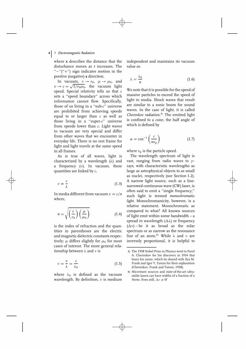
We note that it is possible for the speed ofmassive particles to exceed the speed oflight in media. Shock waves that resultare similar to a sonic boom for soundwaves. In the case of light, it is calledCherenkov radiation.3) The emitted lightis confined to a cone, the half angle ofwhich is defined by

α = cos−1

(c

nvp

)(1.7)

where vp is the particle speed.The wavelength spectrum of light is

vast, ranging from radio waves to γ -rays, with characteristic wavelengths aslarge as astrophysical objects to as smallas nuclei, respectively (see Section 1.2).A narrow light source, such as a line-narrowed continuous wave (CW) laser, isoften said to emit a ‘‘single frequency;’’such light is termed monochromaticlight. Monochromanicity, however, is arelative statement. Monochromatic ascompared to what? All known sourcesof light emit within some bandwidth – aspread in wavelength (�λ) or frequency(�ν) – be it as broad as the solarspectrum or as narrow as the resonanceline of an atom.4) While λ and ν areinversely proportional, it is helpful to

3) The 1958 Nobel Prize in Physics went to PavelA. Cherenkov for his discovery in 1934 thatbears his name, which he shared with Ilya M.Frank and Igor Y. Tamm for their explanation(Cherenkov, Frank and Tamm, 1958).

4) Microwave sources and state-of-the-art ultra-stable lasers can have widths of a fraction of aHertz. Even still, �ν �= 0!

1.1 Introduction 5

Rays

Wave fronts

Optical axis

Refracted ray

Paraxial rayN

onpa

raxi

al ra

y

(a) (b)

α

Fig. 1.1 Definition of rays and wave fronts (a) and paraxialrays (b) where α � 1 rad.

recognize that

∣∣∣∣�λ

λ

∣∣∣∣ =∣∣∣∣�ν

ν

∣∣∣∣ (1.8)

Classically, the treatment of light fallsinto two categories: geometrical andphysical optics. In geometrical optics,the wave properties (e.g., diffraction)are ignored. Conceptually, we let λ → 0and instead discuss rays. While we donot review the usage of rays in thischapter, we do point out that ray tracingis employed extensively for designingoptical systems. Rays are related to wavesin that they are perpendicular linesjoining the wave fronts (see Figure 1.1).The wave fronts turn out to be thesurfaces of constant phase and so rayspoint in the direction of energy flow.Thus, rays from a point source areradial lines perpendicular to sphericalsurfaces. Typically, when dealing withrays, we focus on a subset of all the rayscalled paraxial rays. These rays are nearlyparallel or form a small angle abouta preferred direction. In the exampleshown in Figure 1.1, the ray traversingthe center of the lens is the preferreddirection and is called the optical axis.Paraxial rays deviate from the optical

axis by such a small amount that sin α �tan α � α. Rays are useful for describingrefraction, the bending or redirection oflight at the interface between two mediawith different indices of refraction, andreflection. Refraction, responsible forfocusing of light by lenses and theangular spread of the �λ componentsafter passing through prisms, is aresult of momentum conservation andis succinctly stated through Fermat’sprinciple: light traverses a path from Ato B that is an extremum of the optical pathlength (OPL).5) That is,

δ(OPL) ≡ δ

(∫ B

An(s)ds

)= 0 (1.9)

where s is the geometric path. Fermat’sPrinciple leads to two important proper-ties of light. First, the law of reflection,

θi = θr (1.10)

5) The principle is often stated as the shortestpath, that is, δ(OPL) would be a minimum.However, the calculus of variation only usesthe fact that OPL is stationary; the secondderivative is not considered. Thus, whileusually the case, the path taken is notnecessarily the minimum optical path.


where θi (θr) is the incident (reflected)angle. The second is Snell’s Law,

n1 sin θ1 = n2 sin θ2 (1.11)

relating the incident (θ1) and refracted(θ2) angles for a ray refracted (i.e., bent)as it passes through an interface betweentwo media with different indices ofrefraction.

It is interesting to note that Fermat’sprinciple (ca 1657) is closely related toMaupertu’s principle in mechanics (ca1744) for self-contained systems obeyingconservation laws,

δ

(∫ B

Apds

)= 0 (1.12)

where p is the momentum. Equa-tion (1.12) is the principle of least action6)

when formulated more generally as

δ

(∫ B

AL dt

)= 0 (1.13)

with L being the Lagrangian.7) Theseequations show that particles and raysof light assume rectilinear motions infree space or when there are no forces(fields8)) and the index of refraction isconstant. In general, the trajectories ofparticles and light are stationary. Theindex of refraction plays the role of a field

6) Like with Fermat’s principle, least action isa bit of a misnomer; stationary action wouldbe more appropriate as again only the firstderivative is considered.

7) We point out that Hamilton, Lagrange, Eulerand others played a role in the development ofthe principle as well.

8) Even in vacuum, the trajectory of light isdeflected by a gravitational field. See, forexample, Refs. Misner, Thorne and Wheeler(1973) and Hartle (2003) for a discussion oflight in a gravitational field.

causing rays to deviate from linearitywhen not constant just like forces(potentials) cause particle trajectories tobend.

The geometrical approximation isgood when the variation of the physi-cal features of the media are large incomparison to λ. When they becomecomparable to λ, the wave propertiesof the light must be considered. Therealm of physical optics allows descrip-tions of elements such as apertures andgrating. It further provides a frameworkto discuss fundamental concepts such asdiffraction (the angular spread of a beamof light and the bending of light aroundobstacles Section 1.7), interference (thesuperposition of two or more waves,leading to constructive and destructivesums depending on the relative phaseof the waves Section 1.8), and coherence(issues associated with how stable thephase is in time and across wave fronts).

The smallest unit of light is called thephoton, light quanta after the GermanLichtquanten meaning portions of light.9)

While centuries before the age of quan-tum physics, Isaac Newton championedthe idea of light as a stream of cor-puscles, photons are quantum entitieswhose behavior under certain conditionsare well known. However, the answer tothe question ‘‘What is a photon precisely’’continues to be illusive. Over the years,the definitions tend to fall into one ofthree distinct categories:

• a fundamental particle;• an elementary excitation of the EM

field; or• something registered by a

photodetector.

9) Gilbert N. Lewis is given credit for coiningthis name (Lewis, 1926).

1.2 The Spectrum of Light 7

In this chapter, we do not argue for oragainst one view over another.

Massless photons, like massive parti-cles, carry both energy, hν, and momen-tum, h/λ, where h is Planck’s constant.However, the photon wavefunction mustbe constructed with care. There havebeen suggestions that the photon can beunderstood as simply a classical field plusvacuum fluctuations10) – a semiclassicalapproach if you will. There are cases,however, where such an approach givesthe wrong answer (as determined by ex-perimental observation). Thus, we havetwo regimes: classical light and quantumlight. By definition, quantum light is anybehavior of light that cannot be explainedby classical fields, that is, solutions tothe wave equation. An example wouldbe squeezed light (Henry and Glotzer,1988).

The photon is considered to be afundamental particle. It has an intrinsicspin, which is an integer of unitmagnitude. Thus, it obeys Bose statistics,but it has only two states of helicity(aligned or antialigned with its directionof propagation) because being massless,it has no vacuum rest frame. In additionto spin, light has other nonclassicalfeatures, typically revealing themselvesthrough intensity noise, correlations, andcounting statistics. Finally, both classicalfields as well as photons can carry orbitalangular momentum and support vorticesand solitons (Desyatnikov, Kivshar andTorner, 2005; Kivsha and Agrawol, 2003;Pismen, 1999).

We conclude this introduction bypointing out that if we substitute h/λ

for p into Eq. (1.12), we get a different

10) Vacuum fluctuations refer to the photons thatare created spontaneously from the vacuum.

formulation of Fermat’s principle,

δ

(h

∫ B

A

ds

λ

)= 0 (1.14)

The close analogy between Eqs (1.12)and (1.14) suggests an intimate con-nection between matter and light, fromwhich one can postulate a wave equationfor matter similar to that for light. Aswe discuss in Section 1.9, if we iden-tify the wavelength of the particle ash/p (the de Broglie wavelength) andthe index of refraction with (U − V)/U,where U and V are the total andpotential energies, respectively, thetime-independent Schrodiger equationemerges in a form that is not very dif-ferent from the wave equation for light.Thus, photons, like matter, exhibit bothwave and particle behavior.

With this overview as a backdrop, theremainder of this chapter is devoted tothe details of selected characteristics oflight. We start with the description ofEM spectrum in Section 1.2 followedby a review of the wave equationand its solutions in Section 1.3. InSection 1.4, we consider radiometricissues and address the vector natureof light in Sections 1.5 and 1.6. Wecover diffraction and interference inSections 1.7 and 1.8 and conclude thechapter by further discussing the photonmatter analogy in Section 1.9.

1.2The Spectrum of Light

The EM spectrum is traditionally di-vided into the seven regions shown inFigure 1.2. It should be understood thatthe boundaries between these regionsas well as those between subregions are


100 102 104 106 108 1010 1012 1014 1016 1018 1020 1022 1024

108 106 104 102 100 10−2 10−4 10−6 10−8 10−10 10−12 10−14 10−16

Wavelength (m)

Frequency (× 3 Hz)

Rad

io W

aves

Mic

row

ave

Infr

ared

Vis

ible

Ultr

avio

let

X-r

ays

γ-ra

ys

Fig. 1.2 The electromagnetic radiation spectrum.

not hard and fast, nor are the number ofsubregions unique. The most familiar re-gion of the spectrum, the visible region,consists of wavelengths that range fromabout 0.40 µm at the blue end to 0.78 µmat the red end. Table 1.1 shows the corre-sponding colors for the wavelengths be-tween. The visible subregions are a goodexample of the nonuniqueness of sub-bands of regions; for example, some ref-erences include cyan between green andblue while others insert indigo betweenblue and violet. Breaking the spectruminto six rather than seven or eight bandsis of little consequence typically, becausemost objects emit a range of colors (i.e.,�λ is relatively broad) or multiple colors(e.g., λ1 + λ2 + · · · + λn again spanninga large �λ), making the identification

of a pure color a rare event. Of course,when �λ is small as it often is for somelasers, our eyes in fact do perceive apure color. For example, consider the redHelium–Neon laser at 632.8 nm or thegreen doubled Nd : YAG laser at 532 nm.

Subbands also exist for the otherregions of the EM spectrum. Tables 1.2–1.4 give some of the more familiar sub-bands for the other regions. More aboutthe spectrum of light can be found inRef. (HyperPhysics, 2006).

1.3Basics of Electromagnetic Waves

As mentioned in the introduction,physical optics is concerned with the

Tab. 1.1 The approximate wavelength, frequency, and energyranges for six primary visible color bands. Energies increasefrom left to right.

Color Wavelengths(nm)

Frequencies(×1014 Hz)

Energies(eV)

Red 780–625 3.8–4.8 1.6–2.0Orange 625–590 4.8–5.1 2.0–2.1Yellow 590–565 5.1–5.3 2.1–2.2Green 565–500 5.3–6.0 2.2–2.4Blue 500–435 6.0–6.9 2.4–2.8Violet 435–380 6.9–7.9 2.8–3.6

1.3 Basics of Electromagnetic Waves 9

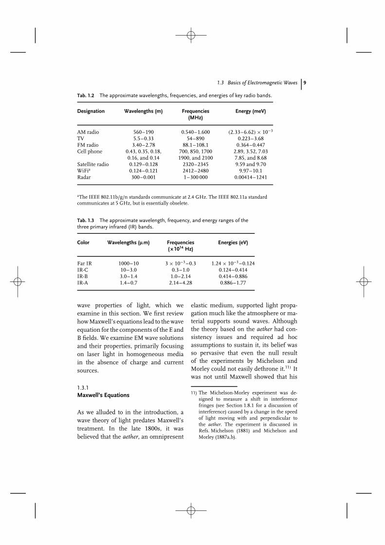
Tab. 1.2 The approximate wavelengths, frequencies, and energies of key radio bands.

Designation Wavelengths (m) Frequencies(MHz)

Energy (meV)

AM radio 560–190 0.540–1.600 (2.33–6.62) × 10−3

TV 5.5–0.33 54–890 0.223–3.68FM radio 3.40–2.78 88.1–108.1 0.364–0.447Cell phone 0.43, 0.35, 0.18, 700, 850, 1700 2.89, 3.52, 7.03

0.16, and 0.14 1900, and 2100 7.85, and 8.68Satellite radio 0.129–0.128 2320–2345 9.59 and 9.70WiFia 0.124–0.121 2412–2480 9.97–10.1Radar 300–0.001 1–300 000 0.00414–1241

aThe IEEE 802.11b/g/n standards communicate at 2.4 GHz. The IEEE 802.11a standardcommunicates at 5 GHz, but is essentially obselete.

Tab. 1.3 The approximate wavelength, frequency, and energy ranges of thethree primary infrared (IR) bands.

Color Wavelengths (µm) Frequencies(×1014 Hz)

Energies (eV)

Far IR 1000–10 3 × 10−3 –0.3 1.24 × 10−3 –0.124IR-C 10–3.0 0.3–1.0 0.124–0.414IR-B 3.0–1.4 1.0–2.14 0.414–0.886IR-A 1.4–0.7 2.14–4.28 0.886–1.77

wave properties of light, which weexamine in this section. We first reviewhow Maxwell’s equations lead to the waveequation for the components of the E andB fields. We examine EM wave solutionsand their properties, primarily focusingon laser light in homogeneous mediain the absence of charge and currentsources.

1.3.1Maxwell’s Equations

As we alluded to in the introduction, awave theory of light predates Maxwell’streatment. In the late 1800s, it wasbelieved that the aether, an omnipresent

elastic medium, supported light propa-gation much like the atmosphere or ma-terial supports sound waves. Althoughthe theory based on the aether had con-sistency issues and required ad hocassumptions to sustain it, its belief wasso pervasive that even the null resultof the experiments by Michelson andMorley could not easily dethrone it.11) Itwas not until Maxwell showed that his

11) The Michelson-Morley experiment was de-signed to measure a shift in interferencefringes (see Section 1.8.1 for a discussion ofinterference) caused by a change in the speedof light moving with and perpendicular tothe aether. The experiment is discussed inRefs. Michelson (1881) and Michelson andMorley (1887a,b).


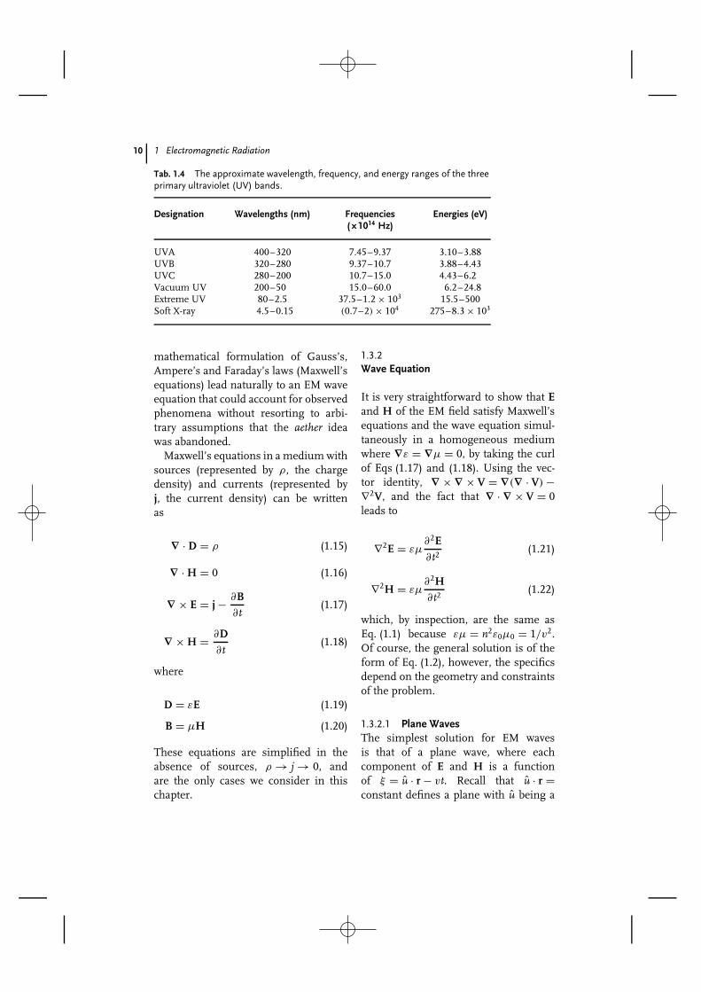
Tab. 1.4 The approximate wavelength, frequency, and energy ranges of the threeprimary ultraviolet (UV) bands.

Designation Wavelengths (nm) Frequencies(×1014 Hz)

Energies (eV)

UVA 400–320 7.45–9.37 3.10–3.88UVB 320–280 9.37–10.7 3.88–4.43UVC 280–200 10.7–15.0 4.43–6.2Vacuum UV 200–50 15.0–60.0 6.2–24.8Extreme UV 80–2.5 37.5–1.2 × 103 15.5–500Soft X-ray 4.5–0.15 (0.7–2) × 104 275–8.3 × 103

mathematical formulation of Gauss’s,Ampere’s and Faraday’s laws (Maxwell’sequations) lead naturally to an EM waveequation that could account for observedphenomena without resorting to arbi-trary assumptions that the aether ideawas abandoned.

Maxwell’s equations in a medium withsources (represented by ρ, the chargedensity) and currents (represented byj, the current density) can be writtenas

∇ · D = ρ (1.15)

∇ · H = 0 (1.16)

∇ × E = j − ∂B∂t

(1.17)

∇ × H = ∂D∂t

(1.18)

where

D = εE (1.19)

B = µH (1.20)

These equations are simplified in theabsence of sources, ρ → j → 0, andare the only cases we consider in thischapter.

1.3.2Wave Equation

It is very straightforward to show that Eand H of the EM field satisfy Maxwell’sequations and the wave equation simul-taneously in a homogeneous mediumwhere ∇ε = ∇µ = 0, by taking the curlof Eqs (1.17) and (1.18). Using the vec-tor identity, ∇ × ∇ × V = ∇(∇ · V) −∇2V, and the fact that ∇ · ∇ × V = 0leads to

∇2E = εµ∂2E∂t2

(1.21)

∇2H = εµ∂2H∂t2

(1.22)

which, by inspection, are the same asEq. (1.1) because εµ = n2ε0µ0 = 1/v2.Of course, the general solution is of theform of Eq. (1.2), however, the specificsdepend on the geometry and constraintsof the problem.

1.3.2.1 Plane WavesThe simplest solution for EM wavesis that of a plane wave, where eachcomponent of E and H is a functionof ξ = u · r − vt. Recall that u · r =constant defines a plane with u being a

1.3 Basics of Electromagnetic Waves 11

dimensionless unit vector perpendicularto that plane. It is straightforward thento show that

∂E∂t

= − v∂E∂ξ

(1.23)

∇ × E = u × ∂E∂ξ

(1.24)

and similarly for H. Because E andH must satisfy Eqs (1.15)–(1.18) (againassuming a homogeneous medium), wecan further write

u × ∂E∂ξ

=√

µ

ε

∂H∂ξ

(1.25)

u × ∂H∂ξ

= −√

ε

µ

∂E∂ξ

(1.26)

Integrating Eqs (1.25) and (1.26) and set-ting the constant to zero (no contributionfrom the background) leads to

E = −√

µ

εu × H (1.27)

H =√

ε

µu × E (1.28)

This implies that E, H, and u form aright-handed orthogonal triad and thatlight is a transverse field, that is, Eand H oscillate in a plane normal tothe propagation direction, in homoge-neous media (including vacuum) with-out sources.

1.3.2.2 Scalar Harmonic WavesThe most common building block forthe EM wave is a wave that is har-monic in both time and space. Theseexhibit sinusoidal variation. Typically, ascalar wave can be expressed as either

a real quantity12)

�(r, t)=A(r, t) cos(k · r ± ωt +ϕ) (1.29)

or a complex quantity,

�(r, t) = A(r, t)ei(k·r±ωt+ϕ) (1.30)

where A is an amplitude that is a slowlyvarying function of position and time(compared with the rapid variation of thesinusoidal arguments), k is the wavevec-tor (|k| = 2π/λ) and ω (= 2πν) is theangular frequency. Now it should be clearthat u. The harmonic time dependenceof the wave allows the wave equation tobe written as

∇2ψ + k2ψ = 0 (1.31)

Because E and B are vectors, the EM waveis actually a vector wave. Generally, eachcomponent of the field satisfies the waveequation (Eq. 1.31) and has solutions likethose in Eq. (1.29) and (1.30).

The argument of the harmonic waveconsists of two phase terms, ξ± ≡ k · r ±ωt, the dimensionless version of ξ , andϕ. A constant ξ− (ξ+) defines a profileor phase of the wave that moves towardmore positive (negative) r as time evolvesat a speed

v = ω

|k| (1.32)

known as the phase velocity. The secondphase term is often referred to as therelative phase of the wave. It can bea fixed constant or time dependent.When it is a constant or has a welldefined time dependence, it gives rise

12) Note, we have multiplied ξ by |k| (|k|v = ω

because |k| = nω/c) to make the argumentdimensionless.


to coherence. When it varies randomlywith time, the light is said to beincoherent. Furthermore, when ϕ(t) =const·tn, the frequency changes withtime. A linear dependence simply shiftsthe frequency while higher powers chirpthe frequency – as the wave passes thefrequency either increases or decreases,depending on the sign of the constant.More complicated functions are possibleas well.

1.3.2.3 Waves with Curved Phase FrontsAlthough plane waves are highly conve-nient to use, they are appropriate onlywhen dealing with light that is effectivelyfar from its source.13) Many situationsdo not fall into this category. It is beyondthe scope of this chapter to discuss non-planar waves extensively, but we will givetwo examples. For a more extensive dis-cussion, the reader is directed to the textby Cowan, 1968. First, when the frontsare not planes, the solutions in Eq. (1.30)must be modified to correspond to theLaplacian being expressed in a differ-ent coordinate system. For example, aspherical wave takes the form

�(r, t) = A

rei(kr±ωt+ϕ) (1.33)

where kr = constant. The phase fronts areclearly spheres. A bit more complicatedexample would be a cylindrical wave,which follows

�(ρ, z, θ, t)

= AJm(kρ)e±ikzze±imθ e−i(ωt+ϕ) (1.34)

where Jm(kρ) is the mth order Besselfunction of the first kind (which are

13) By far field, we mean that the phase fronts areplanes. This can be achieved near the sourcewith lenses.

regular at the origin)14) with m beinga positive integer, and

k2 =(ω

c

)2 + k2z (1.35)

The surfaces of constant phase are justcylinders in this case.

1.4Energy, Intensity, Power, and Brightness

Because the EM field is composed of Eand B fields, its Energy Density is given by

u = 1

2

(ε|E|2 + µ|H|2) (1.36)

As a wave, this energy flows as describedby the Poynting Vector,

S = E × H (1.37)

The Intensity of the light is defined as thetime average of S,

I = |〈S〉| ≡ 1

2|E × H| = n

2µc|E|2 (1.38)

which has dimensions of watt per squarecentimeter.15) In Eq. (1.38) we used thefact that ω/|k| = c/n. In vacuum, usingthe fact that ε0µ0 = 1/c2, we can write

I = 1

2µ0c|E|2 = 1

2ε0c|E|2 (1.39)

� |E|2240π

(1.39a)

14) The boundary conditions of the problemmight dictate a different Bessel solution.For example, if the origin were excluded,Bessel functions of the second kind, whichare singular at the origin, would have to beconsidered as well.

15) Technically, the SI unit is watt per squaremeter but in the United States, it is typicallyexpressed as watt per square centimeter .

1.5 Polarization 13

In this form, I has dimensions of wattper square centimeter (watt per squaremeter) when the dimensions of E arevolt per centimeter (volt per meter).The Power, P, delivered is the integratedintensity over the exposed area,

I = P

A(1.40)

where A is the area.16) A related quantity,the Brightness, which is sometimesreferred to as the Radiance, takes intoaccount the solid angle, ��, throughwhich the intensity is delivered and isgiven by

B = I

��(1.41)

which has dimensions watts per stera-dian per square centimeter. It is inter-esting to note that an unfocused laserdelivering 1 mW of power at 780 nmis considerably brighter than a 100 Wlight bulb, 1.7 × 107 W/sr-cm2 for a typi-cal laser beam17) with w0 = 1 mm and�� = 2 × 10−7 sr compared with 0.6W/sr-cm2 for a light bulb at a distanceof 1 m radiating into 4π . Thus, a laser isconsidered very bright, which can do realdamage to an unprotected eye. Finally,laser light can be further characterizedby its spectral brightness, the brightnessper unit optical bandwidth,

SB = B

�ν(1.42)

with units as watts per steradian persquare centimeter hertz. The brightnessand spectral brightness are often confused

16) The area of a laser beam is given by πw20,

where w0 is the beam radius.17) For a diffraction limited laser beam, �� =

πθ2d where θd = λ/πw0.

with each other as well as with theLuminance, a photometric quantity re-ferring to a perceived brightness relatedmore to how the eye responds.

1.5Polarization

As mentioned earlier, EM waves areactually vector waves, because E and Bpoint in specific directions. Polarizationcaptures this feature, and is defined interms of the direction of E.18) The mostgeneral case is elliptical polarization,which has two limiting cases, linearand circular polarization. These namesare so chosen because they describethe geometric shapes E that sweeps outwhile looking at the light along (parallelor antiparallel to) k. We have alreadydiscussed that E, B, and k form a right-handed Cartesian triad so polarizationalso specifies the direction of B. We willtake k ≡ z and focus on light that isperfectly polarized in the discussion thatfollows.

In general E will have two orthogonalcomponents,

E1 = xE01ei(kz−ωt+ϕ1)

= xE01ei(ξ+ϕ1) (1.43)

E2 = yE02ei(kz−ωt+ϕ2)

= yE02ei(ξ+ϕ2) (1.44)

We will first consider the case whereE01, E02, ϕ1, and ϕ2 are all real and

18) Another reason for considering only E is themagnitude of B relative to E is down by a factorof c. Thus at low intensities, < 1014 W/cm2, Edominates the physics.


Tab. 1.5 Various electromagnetic field quantities.

Quantity Name SI Unit

c = 2.99792458 × 108 Light vacuum speeda m/sµ0 = 4π × 10−7 Vacuum permeabilitya T-m/A (kg-m/A2-s2)ε0 = 8.854187817 . . . × 10−7 Vacuum permittivity F/m (A2-sec4/kg-m3)E Electric fieldb V/m (kg-m/A-s3)D Electric displacement C/m2

B Magnetic inductionc T (kg/A-s2)H Magnetic field A/mρ Charge densityb C/m3

j Current densityb A/m2

P Power W (kg/m2-s3)S ≡ E × H Poynting vector W/m2 (kg/m4-s3)I ≡ 〈|S|〉 Intensityb W/cm2

a All defined to be exact.b In the US, the explicit length measures for these quantities are given in centimeters, forexample, volt per centimeter, watt per square centimeter, and so on.c Sometimes called the magnetic-flux density.

time independent. Taking the real partof these fields,

E1 = xE01 cos(ξ + ϕ1) (1.45)

E2 = yE02 cos(ξ + ϕ2) (1.46)

leads to an equation of a conic section

( |E1|E01

)2

+( |E2|

E02

)2

− 2( |E1|

E01

) ( |E2|E02

)cos ϕ=sin2 ϕ (1.47)

and ϕ=ϕ2 − ϕ1. Equation (1.47) de-scribes an ellipse when

sin2 ϕ

E201E2

02

≥ 0 (1.48)

Because the numerator and denominatorare positive definite, Eq. (1.48) is alwaystrue.

Special Linear Case # 1: ϕ = 0 or ϕ = π

Equation (1.47) reduces to

|E1|E01

= |E2|E02

(1.49)

which describes a straight line. Becausethe two component oscillate in phase,this case leads to linear polarization. Thecase for ϕ = 0 and ϕ = π are orthogonalto each other.

Special Circular Case # 2: ϕ = ±π/2 andE01 = E02

The equation reduces to

|E1|2 + |E2|2 = E201 (1.50)

the equation of a circle of radius E01.The two components are out of phaseby half a wavelength (or period) butthe magnitude of the resultant, E01, isconstant but sweeps out a circle leadingto circular polarization. The sense ofrotation depends on the sign of ϕ,

1.5 Polarization 15

with the minus (plus) sign producinglight with positive (negative) helicity,where positive helicity obeys the right-hand rule, so if you look in thedirection of propagation, the E-fieldrotates clockwise.19)

Special Elliptical Case # 3: ϕ = ±π/2 andE01 �= E02

Equation (1.47) reduces to

( |E1|E01

)2

+( |E2|

E02

)2

= 1 (1.51)

which is an ellipse with the major axisaligned with the horizontal (vertical) axiswhen E01 > E02 (E01 < E02). The sense ofrotation is the same as in special case # 2.

General Elliptical Case E01 �= E02

In the general elliptical polarization case,one has a rotated ellipse where the angle,α, of the major axis away from the E1

direction is given by

tan 2α = 2E01E02

E201 − E2

02

cos ϕ (1.52)

Note, when E01 = E02, Eq. (1.52) cannotbe used and one must go back toEq. (1.47) to determine α.

1.5.1Polarization Bookkeeping

There are several approaches to keepingtrack of the polarization of light, which isparticularly important when light inter-acts with media that can either decreasethe intensity or delay the transit time of

19) It should be noted that some referencesdefine circular polarization in terms of right-hand and left-hand circular polarization. Thisdefinition traditionally corresponds to lookingantiparallel to k so ϕ = −π/2 would lead toleft-hand circular polarization.

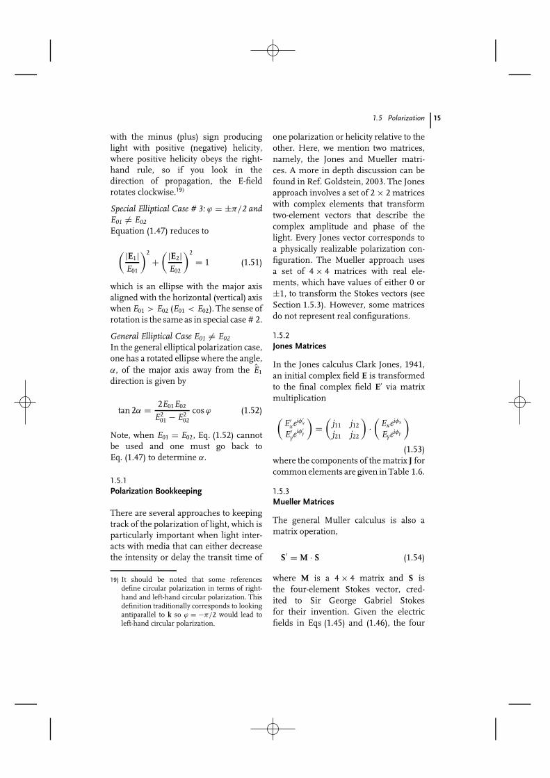
one polarization or helicity relative to theother. Here, we mention two matrices,namely, the Jones and Mueller matri-ces. A more in depth discussion can befound in Ref. Goldstein, 2003. The Jonesapproach involves a set of 2 × 2 matriceswith complex elements that transformtwo-element vectors that describe thecomplex amplitude and phase of thelight. Every Jones vector corresponds toa physically realizable polarization con-figuration. The Mueller approach usesa set of 4 × 4 matrices with real ele-ments, which have values of either 0 or±1, to transform the Stokes vectors (seeSection 1.5.3). However, some matricesdo not represent real configurations.

1.5.2Jones Matrices

In the Jones calculus Clark Jones, 1941,an initial complex field E is transformedto the final complex field E′ via matrixmultiplication

(E′

xeiφ′x

E′ye

iφ′y

)=

(j11 j12

j21 j22

)·(

Exeiφx

Eyeiφy

)(1.53)

where the components of the matrix J forcommon elements are given in Table 1.6.

1.5.3Mueller Matrices

The general Muller calculus is also amatrix operation,

S′ = M · S (1.54)

where M is a 4 × 4 matrix and S isthe four-element Stokes vector, cred-ited to Sir George Gabriel Stokesfor their invention. Given the electricfields in Eqs (1.45) and (1.46), the four


Tab. 1.6 Jones matrices for common opticalelements.

Optical element Jones matrix

Linear polarizer ‖x

(1 00 0

)

Linear polarizer ‖y

(0 00 1

)

Linear polarizer at ±45◦ 12

(1 ±1

±1 1

)14 -Wave plate, Fast axis

‖ x (+)

y (−)

eiπ/4

(1 00 ±i

)

Circular polarizer,± Helicity

eiπ/4

(1 ∓i±i 1

)

components of S are defined as

S0 = |E01|2 + |E02|2 (1.55)

S1 = |E01|2 − |E02|2 (1.56)

S2 = |2E01E02 cos ϕ| (1.57)

S3 = |2E01E02 sin ϕ| (1.58)

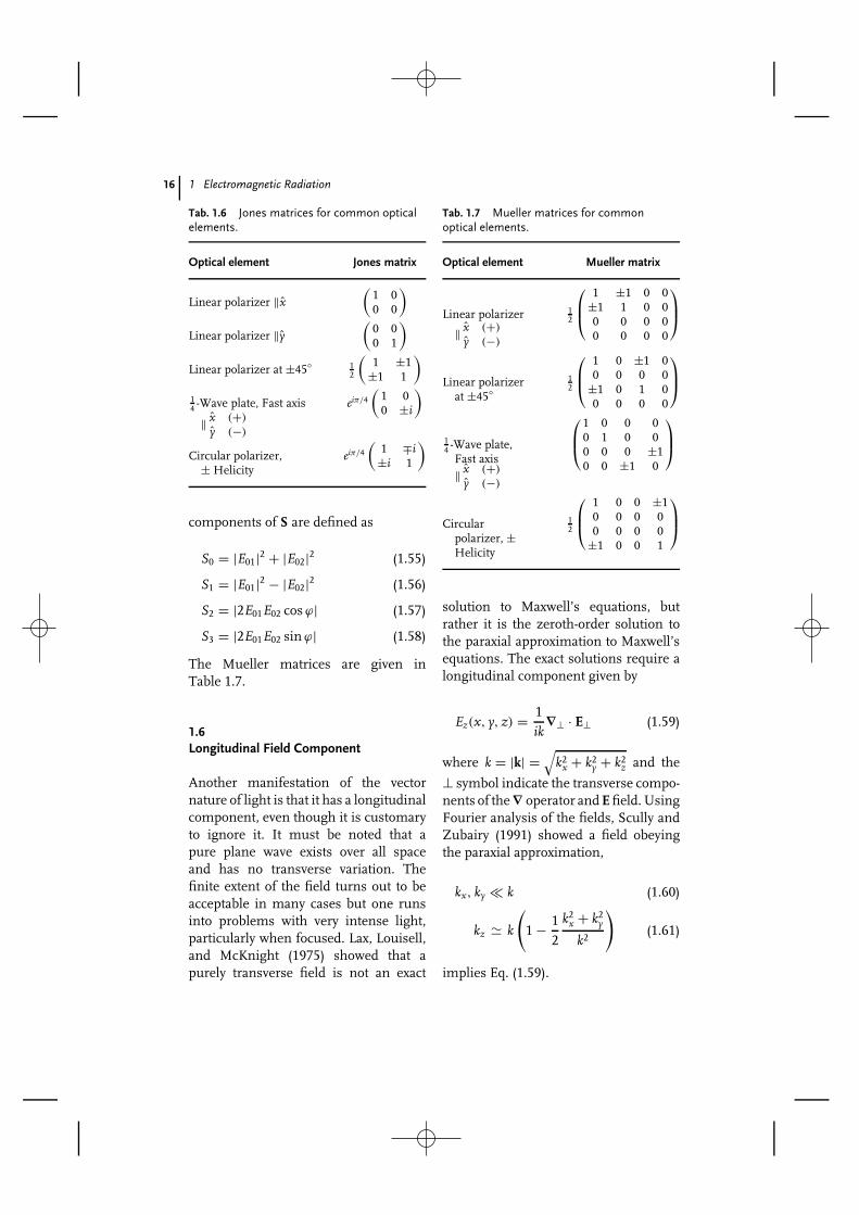
The Mueller matrices are given inTable 1.7.

1.6Longitudinal Field Component

Another manifestation of the vectornature of light is that it has a longitudinalcomponent, even though it is customaryto ignore it. It must be noted that apure plane wave exists over all spaceand has no transverse variation. Thefinite extent of the field turns out to beacceptable in many cases but one runsinto problems with very intense light,particularly when focused. Lax, Louisell,and McKnight (1975) showed that apurely transverse field is not an exact

Tab. 1.7 Mueller matrices for commonoptical elements.

Optical element Mueller matrix

Linear polarizer

‖ x (+)

y (−)

12

1 ±1 0 0±1 1 0 00 0 0 00 0 0 0

Linear polarizerat ±45◦

12

1 0 ±1 00 0 0 0

±1 0 1 00 0 0 0

14 -Wave plate,

Fast axis‖ x (+)

y (−)

1 0 0 00 1 0 00 0 0 ±10 0 ±1 0

Circularpolarizer, ±Helicity

12

1 0 0 ±10 0 0 00 0 0 0

±1 0 0 1

solution to Maxwell’s equations, butrather it is the zeroth-order solution tothe paraxial approximation to Maxwell’sequations. The exact solutions require alongitudinal component given by

Ez(x, y, z) = 1

ik∇⊥ · E⊥ (1.59)

where k = |k| =√

k2x + k2

y + k2z and the

⊥ symbol indicate the transverse compo-nents of the ∇ operator and E field. UsingFourier analysis of the fields, Scully andZubairy (1991) showed a field obeyingthe paraxial approximation,

kx, ky � k (1.60)

kz � k

(1 − 1

2

k2x + k2

y

k2

)(1.61)

implies Eq. (1.59).

1.7 Diffraction 17

1.7Diffraction

When light passes a sharp edge, it doesnot produce a sharp shadow. Also, whenit passes through a circular hole, itdoes not produce a disk of the samesize. Under the right conditions, it pro-duces not only a larger spot but alsorings. Furthermore, the transverse sizeof a laser beam expands as it propa-gates. These observations are elegantlydescribed by diffraction theory. Diffrac-tion falls into two classes – Fraunhoferand Fresnel. Fraunhofer diffractions de-scribes what happens when the phasefronts are near plane waves, where thecurvature of the field can be ignored.Fresnel diffraction takes curvature intoaccount.

Huygens, in the late seventeenthcentury, suggested a description for wavepropagation as a collection of individualspherical sources called secondary sources,the sum of which would make up thewavefront. It is a straightforward exerciseto convince oneself that Huygens’sprinciple can be used to construct aplane as well as other simple geometries.When applied to a hole, Huygens’sapproach leads to an emerging sphericalwave, because part of the plane wave isblocked. This would appear to accountfor the observed spread. However, thereis a difficulty. If the secondary wavesare spherical, then there should alsobe part of the wave going backward.Huygens had to ignore this part of thewave. It turns that when consideredmore mathematically, this problem iscorrected by what is call the obliquityfactor.

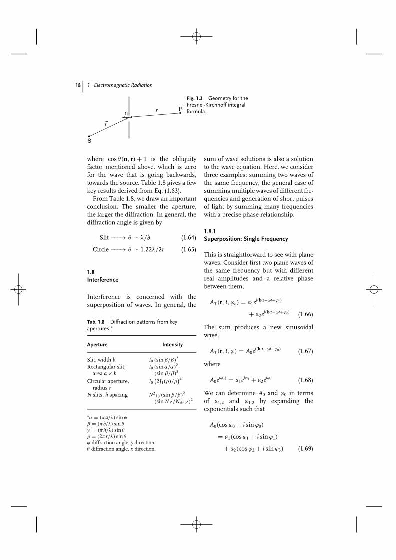
The mathematical statement of theprinciple for a wave propagating infree space is the Fresnel-Kirchhoff

integral formula,20)

ψP = − ik

4πψ0

∫ ∫eik(r+r)

rr

× [cos θ(n, r) − cos θ(n, r)] dA

(1.62)where the integral is over the area of theaperture. The distances, r and r, betweenthe aperture and observation point andaperture and source, respectively, are de-fined in Figure 1.3 as is n, the normal tothe surface, pointing toward the source.The angles between the vectors and thenormal are represented by θ(n, r) andθ(n, r).

Let’s consider an example of anaperture. In the Fraunhofer limit, s andp are effectively a long way from theaperture. In this case, we can take thesurface of the aperture to be a sphericalcap such that F is constant. Thus, r and nare antiparallel always and cos θ(n, r) =−1.21) Equation (1.62) then reduces to

ψP = − ik

4πAψ0

∫eik(r+r)

rr

× [cos θ(n, r) + 1] dA (1.63)

20) The Fresnel-Kirchhoff integral formula ofEq. (1.62) can be derived from Green’stheorem (see, for example, Fowles, 1968) fortwo functions that are continuous, integrableand satisfy the wave equation,

∫ ∫(V∇⊥U − U∇⊥V) dA

=∫ ∫ ∫ (

V∇2U − U∇2V)

dV

where the first integral is over any closedsurface and the second is over the volumeenclosed.

21) When r and r are much larger than theaperture size, a spherical surface is not muchdifferent from a flat surface.


S

P

r

n r

Fig. 1.3 Geometry for theFresnel-Kirchhoff integralformula.

where cos θ(n, r) + 1 is the obliquityfactor mentioned above, which is zerofor the wave that is going backwards,towards the source. Table 1.8 gives a fewkey results derived from Eq. (1.63).

From Table 1.8, we draw an importantconclusion. The smaller the aperture,the larger the diffraction. In general, thediffraction angle is given by

Slit −−−→ θ ∼ λ/b (1.64)

Circle −−−→ θ ∼ 1.22λ/2r (1.65)

1.8Interference

Interference is concerned with thesuperposition of waves. In general, the

Tab. 1.8 Diffraction patterns from keyapertures.∗

Aperture Intensity

Slit, width b I0 (sin β/β)2

Rectangular slit,area a × b

I0 (sin α/α)2

(sin β/β)2

Circular aperture,radius r

I0(2J1(ρ)/ρ

)2

N slits, h spacing N2I0 (sin β/β)2

(sin Nγ /Nsinγ )2

∗α = (πa/λ) sin φ

β = (πb/λ) sin θ

γ = (πh/λ) sin θ

ρ = (2πr/λ) sin θ

φ diffraction angle, y direction.θ diffraction angle, x direction.

sum of wave solutions is also a solutionto the wave equation. Here, we considerthree examples: summing two waves ofthe same frequency, the general case ofsumming multiple waves of different fre-quencies and generation of short pulsesof light by summing many frequencieswith a precise phase relationship.

1.8.1Superposition: Single Frequency

This is straightforward to see with planewaves. Consider first two plane waves ofthe same frequency but with differentreal amplitudes and a relative phasebetween them,

AT(r, t, ϕo) = a1ei(k·r−ωt+ϕ1)

+ a2ei(k·r−ωt+ϕ2) (1.66)

The sum produces a new sinusoidalwave,

AT(r, t, ϕ) = A0ei(k·r−ωt+ϕ0) (1.67)

where

A0eiϕ0) = a1eiϕ1 + a2eiϕ0 (1.68)

We can determine A0 and ϕ0 in termsof a1,2 and ϕ1,2 by expanding theexponentials such that

A0(cos ϕ0 + i sin ϕ0)

= a1(cos ϕ1 + i sin ϕ1)

+ a2(cos ϕ2 + i sin ϕ3) (1.69)

1.8 Interference 19

Equating the cosine (sine) terms on theleft with those on the right and thendividing the sine terms by the cosineterms leads to

tan ϕ0 = a1 sin ϕ1 + a2 sin ϕ2

a1 cos ϕ1 + a2 cos ϕ2(1.70)

At the same time, taking the modulussquared of Eq. (1.68) produces

|A0|2 = |a1|2 + |a2|2+ (

a1a∗2ei�ϕ0 + c.c.

)= a2

1 + a22 + 2a1a2 cos �ϕ0 (1.71)

where �ϕ0 = ϕ1 − ϕ2. Given a1,2 andϕ1,2, A0 (the intensity) and ϕ0 canbe found from Eqs (1.70) and (1.71).Equation (1.71) is known as the coherentsum of the two waves. That is, oneadds the amplitudes before squaringto get the total intensity. The intensityis proportional to the square of theamplitude so it is also possible to writeEq. (1.71) as

IT = I1 + I2 + 2√

I1I2 cos �ϕ0 (1.72)

The third term in (Eqs 1.71 and 1.72)is sometimes called the interference termand plays an important role in describingthe intensity of the resultant wave.Consider the case where a1 = a2 soI1 = I2 = I. When �ϕ0 = 2mπ (m =0, 1, 2, . . .), the two waves are said tobe in phase, in which case

IT = (a1 + a2)2 = 4I (1.73)

When �ϕ0 = (2m + 1)π/2, we have theopposite extreme,

IT = (a1 − a2)2 = 0 (1.74)

When a1 �= a2, the two extremes give re-sultants with maximum and minimumIT respectively.

In the more general case of manywaves, all with the same frequency, wehave

AT(r, t, ϕ0) = A0ei(k·r−ωt+ϕ0)

=N∑

j=1

ajei(k·r−ωt+ϕj) (1.75)

where

IT = |A0|2 =N∑

j=1

|aj|2 + 1

2

N∑j �=k(

aja∗kei(ϕj−ϕk) + c.c.

)(1.76)

and

tan ϕ0 =∑N

j=1 aj sin ϕj∑Nj=1 aj cos ϕj

(1.77)

Again, the resultant is a sinusoidal wavewith an intensity given by a coherentsum. In the case where all the amplitudesare the same so that each wave has anintensity I,

IT = N2I (1.78)

In the case where �j,k = ϕj − ϕk is notwell defined but varies randomly withtime, it is straightforward to show thatthe second sum in Eq. (1.76) vanishesby writing the exponentials in terms ofsines and cosines and using the fact thatthe time average of sin �j,k → 0 as doesthat of cos �j,k. Thus, the interferenceterms vanish. In the case where allamplitudes are the same, the resultantwave corresponds to an incoherent sumof the contributors,

IT = NI (1.79)


For an incoherent sum, one squares firstand then adds the intensities.

1.8.1.1 InterferometryAn entire field of study with industrialapplications is built upon an equationsimilar to Eq. (1.72). The most generalsituation is where a beam of light isdivided into two with each traveling dif-ferent paths and brought back together.Because the two beams came from thesame source, and if the path length dif-ference is not too large, so that the twobeams are still in phase, the resultantintensity will be the same as Eq. (1.72)except that �ϕ0 → δ in the argument ofthe interference term where

δ = k�l (1.80)

with �l being the path length differencebetween the two arms. In this case, con-structive interference occurs when �l =nλ, whereas destructive interference oc-curs when �l = (2n + 1)λ/2, where n isa positive integer. Two-beam interfero-metry exploits interference patterns tomeasure inhomogeneities and defects inmaterial.

1.8.2Superposition: Multiple Frequencies

Superposition involving waves of dif-ferent frequencies leads to some veryinteresting possibilities such as ultra-short busts of light. The general principleof summing waves with different fre-quencies can be understood in the specialcase where the amplitude and phase arethe same for each wave:

AT(r, t) = A0 exp[i(k1 · r − ω1t)]

+ A0 exp[i(k2 · r − ω2t)]

= 2A0 exp

[i

2(�k · r − �ωt)

]

× exp[

i

2(km · r − ωmt)

](1.81)

where

�k = 1

2(k1 − k2) (1.82)

km = 1

2(k1 + k2) (1.83)

�ω = 1

2(ω1 − ω2) (1.84)

ωm = 1

2(ω1 + ω2) (1.85)

Equation (1.81) represents a wave os-cillating at the mean of the two fre-quencies, ωm, and modulated by atemporal and spatial envelope given

by 2A0 exp[i

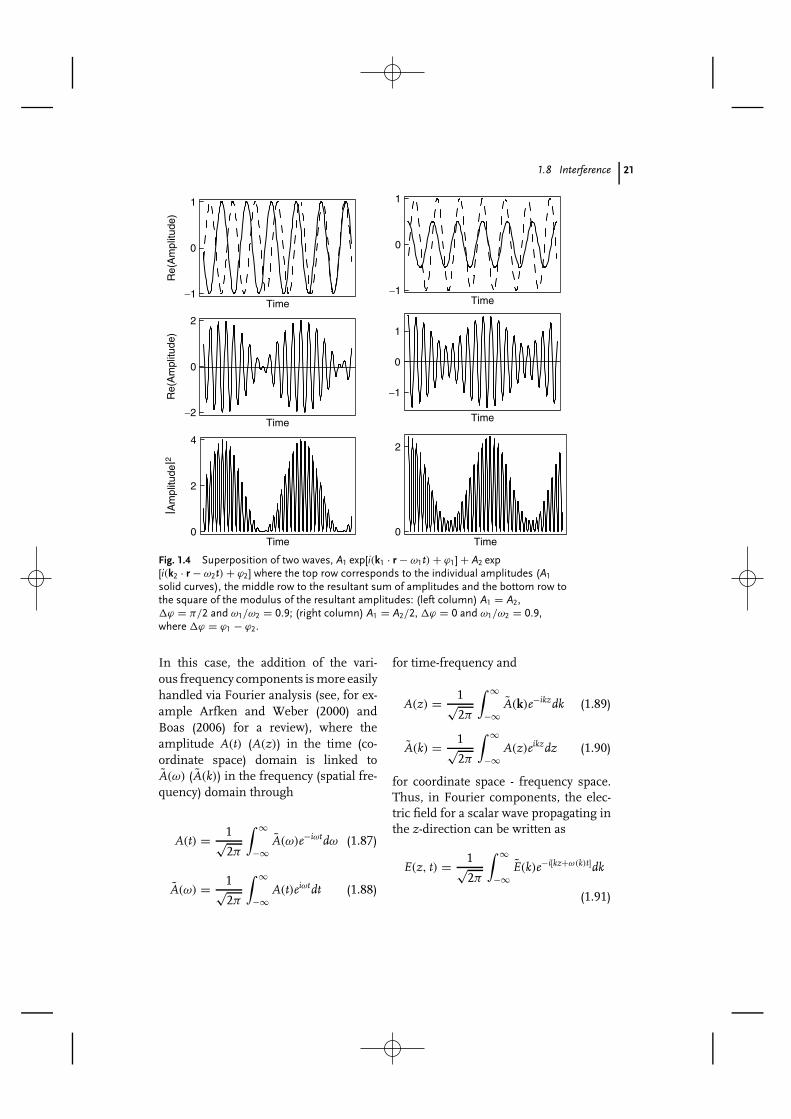
2(�k · r − �ωt)]. Figure 1.4

shows examples of adding two waveswith different frequencies. Unlike thecase of equal frequencies, in this case,the two sinusoidal waves produce a wavethat is periodic but not sinusoidal. Suchwaves are called anharmonic. For thesum of two waves, we have two differ-ent speeds. As with a single frequency,we again have a phase velocity – the ra-tio between the average frequency andwavenumber, vph = ωm/|k|. But, we havea new speed that goes by the name of thegroup velocity, the speed with which theenvelope moves, vg = �ω/�|k|.

When a wave is composed of manyfrequencies, ω → ω(k). Typically, thefrequencies are grouped around a centralfrequency, ω(k0), allowing ω(k) to beexpanded into a Taylor series,

ω(k) = ω(k0) + (k − k0)dω

dk

∣∣∣∣k0

+ · · ·

(1.86)

1.8 Interference 21

Time−1

0

1

Time

−1

0

1

Time0

2

Time0

2

4

Time−2

0

2

Time−1

0

1

Re(

Am

plitu

de)

Re(

Am

plitu

de)

|Am

plitu

de|2

Fig. 1.4 Superposition of two waves, A1 exp[i(k1 · r − ω1t) + ϕ1] + A2 exp[i(k2 · r − ω2t) + ϕ2] where the top row corresponds to the individual amplitudes (A1

solid curves), the middle row to the resultant sum of amplitudes and the bottom row tothe square of the modulus of the resultant amplitudes: (left column) A1 = A2,�ϕ = π/2 and ω1/ω2 = 0.9; (right column) A1 = A2/2, �ϕ = 0 and ω1/ω2 = 0.9,where �ϕ = ϕ1 − ϕ2.

In this case, the addition of the vari-ous frequency components is more easilyhandled via Fourier analysis (see, for ex-ample Arfken and Weber (2000) andBoas (2006) for a review), where theamplitude A(t) (A(z)) in the time (co-ordinate space) domain is linked toA(ω) (A(k)) in the frequency (spatial fre-quency) domain through

A(t) = 1√2π

∫ ∞

−∞A(ω)e−iωtdω (1.87)

A(ω) = 1√2π

∫ ∞

−∞A(t)eiωtdt (1.88)

for time-frequency and

A(z) = 1√2π

∫ ∞

−∞A(k)e−ikzdk (1.89)

A(k) = 1√2π

∫ ∞

−∞A(z)eikzdz (1.90)

for coordinate space - frequency space.Thus, in Fourier components, the elec-tric field for a scalar wave propagating inthe z-direction can be written as

E(z, t) = 1√2π

∫ ∞

−∞E(k)e−i[kz+ω(k)t]dk

(1.91)


In many cases, dω/dk is the appropriateand more general expression for thegroup velocity. This can be seen bysubstituting the first two terms ofEq. (1.86) into Eq. (1.91),

E(z, t) = 1√2π

ei[k0(dω/dk)|k0 −ω(k0)]t

×∫ ∞

−∞E(k)e−i[z+(dω/dk)|k0 t]kdk

(1.92)

However, Eq. (1.90) implies

E(k)= 1√2π

∫ ∞

−∞E(z, t = 0)eikzdz

(1.93)which allows Eq. (1.92) to be written as

E(z, t) = ei[k0(dω/dk)|k0 −ω(k0)]t

2π

×∫ ∞

−∞E(z′, 0)dz′

×∫ ∞

−∞ei(z′−z−(dω/dk)|k0 t)kdk

(1.94)where we do the k integration first. Thelast integral is just δ

(z′ − z − dω

dk

∣∣k0

t),

from which we get

E(z, t) = 1

2πE(z + dω/dk|k0 t, 0)

× e−i[ω(k0)−k0(dω/dk)|k0 ]t (1.95)

By inspection, it is clear that theenvelope in Eq. (1.95) moves with speeddω/dk|k0 and the carrier oscillates withfrequency ω(k0) − k0

dωdk |k0 under the

envelope. Thus, we define the groupvelocity as

vg = dω

d|k| (1.96)

In vacuum vph = vg . However, if themedium through which the wave prop-agates is dispersive, n → n(λ) so thatdn/d|k| �= 0, the two velocities can bevery different. Thus, it is often conve-nient to write vg in a form that includesthe dispersion explicitly,

vg = c

n

(1 − |k|

n

dn

d|k|)

(1.97)

The group velocity is typically the speedwith which information is transmitted. Itis important to remember that the groupvelocity is actually only the first termin a series and in cases where dn/d|k|changes very rapidly or is anomalous(i.e., negative), higher order terms mustbe kept to determine the speed withwhich information travels correctly.

1.8.3Short Pulses

Figure 1.4 shows the basic idea forgenerating pulses of light of shortduration. Specifically, in this case, twofrequencies with well-defined relativephase (i.e., fixed in time) are summedin the frequency domain to provide anew wave with beats in the time domain.As additional frequencies are added, thetemporal width of the beat envelopenarrows. To gain a better understandingof the relationship between the lengthof the pulse train and its bandwidth ornumber of frequencies required to sumin order to produce it, we will turnthe problem around and start with anidealized pulse train in the time domain.Figure 1.5, for example, shows two finitelength, idealized, pulse trains, one withthree cycles and the other with six cycles.

1.8 Interference 23E

(t)

E(t

)

t t

2t 2t

∆w ∆w

E(w

)∼ E(w

)∼

w–w0w–w0

Fig. 1.5 Idealized short pulses formed by finite unit amplitude N-cycle pulsetrains (top) with N = 6 (left) and N = 3 (right). Their respective Fouriertransforms appear below with peak amplitudes of

√π/2N/ω0 and the first zeros

occurring at ω = ω0(1 ± 1/N).

Mathematically, these obey

E(t) ={

E0 sin ω0t for − τ ≤ t ≤ τ

0 at other times.

(1.98)The length of this pulse is 2τ , whereτ = Nπ/ω0 with N being the numberof cycles in the train. Using a Fourieranalysis similar to that described above,the frequency spectrum is given by

E(ω) = E0√2π

[sin τ(ω − ω0)

ω − ω0

− sin τ(ω + ω0)

ω + ω0

](1.99)

At optical or near IR frequencies, be-cause the second term is much smallerthan the first, we can apply the Fouriertransform to just the first term, whichis also plotted in Figure 1.5. Clearly,the number of frequencies involved inthe shorter pulse is larger than the

number needed for the longer pulse.This inverse relationship between thelength of the pulse in the time domainand the spread in the frequency do-main is conveniently captured in thetime-bandwidth product, τ�ν. FromFigure 1.5 and Eqs (1.98) and (1.99), itis clear that E(ω) = 0 when Nπ(ω −ω0)/ω0 = ±π . Thus, �ω = ω+ − ω− =2ω0/N = 2π/τ , where ω± = ω0

(1 ± 1/N), which leads to

τ�ν = 1 (1.100)

It is interesting to note that if we multi-ply Eq. (1.100) by h, this time-bandwidthproduct satisfies the Heisenberg uncer-tainty principle,

�t�E ≥ h

2(1.101)

where �E = h�ν, h = h/2π and wesubstituted �t for τ . The minimum is


reached when the so-called minimumuncertainty wavepacket is prepared.22)

Ultrashort pulses are achieved by‘‘locking’’ the frequency componentsthat extends over a wide frequencyrange. The minimum width achievableby this technique corresponds to onecomplete cycle of light. At 800 nm, nearthe peak of the Ti : Sapphire laser,this is ∼ 2.7 femtoseconds. For a morecomplete discussion on mode lockingand the generation of ultrashort pulses,the reader is directed to the classic textby Siegman Siegman, 1986

1.9Photons and Particles

We conclude by discussing the anal-ogy between light and particle wavesa bit further. Equations (1.13), (1.14)and (1.31) can be used to motivethe time-independent Schrodinger waveequation,

− h2

2m∇2ψ + Vψ = Eψ (1.102)

∇2ψ + 2m

h2 (E − V)ψ = 0 (1.103)

where h = h/2π . Because λ for the par-ticle is h/p, in free space, we postulatethat k (= 2πn/λ) in Eq. (1.31) must beproportional to p. Thus, in the absenceof a potential (when n = 1)

k2n=1 = p2

h2/4π2(1.104)

But,

p2 = 2mE (1.105)

22) The minimum spread criterion applies toconjugate variables such as time frequencyand position momentum.

so

k2n=1 = 2m

h2 E, which lead to Eq. 1.102.

(1.106)To account for the potential we letn2 = (E − V)/E �= 1 so that k2 = n2k2

n=1is just the coefficient of the second termin Eq 1.103.

Space does not permit a more in depthdiscussion of the quantum nature oflight. The interested reader is directedto a recent review Smith and Raymer,2007 and references therein.

References

Arfken, G. and Weber, H. (2000) MathematicalMethods for Physicists, 5th edn, AcademicPress, New York. ISBN 0-12-059825-6.

Boas, M.L. (2006) Mathematical Methods in thePhysical Sciences, 3rd edn, Wiley, New York.ISBN 978-0-471-19826-0.

Cherenkov, P.A., Frank, I.M. and Tamm, I.Y.(1958) Nobel Prize. http://nobelprize.org/nobel prizes/physics/laureates/1958/.

Clark Jones, R. (1941) New calculus for thetreatment of optical systems. I. Descriptionand discussion of the calculus. J. Opt. Soc.Am., 31, 488.

Cowan, E.W. (1968) Basic Electromagnetism,Academic Press, New York. ISBN0-12-193950-2.

Desyatnikov, A.S., Kivshar, Y.S. andTorner, L. (2005) Progress in Optics, Vol. 47,North-Holland, Publishing CompanyAmsterdam, 291–391.

Fowles, G.F. (1968) Introduction to ModernOptics, Holt, Rinehart and Winston, Inc,New York. ISBN 0-03-065365-7.

Glauber, R.J. (2005) Nobel Prize.http://nobelprize.org/nobel prizes/physics/laureates/2005/glauber-lecture%.html.

Goldstein, D. (2003) Polarized Light, 2nd edn,Marcel Dekker, Inc., New York. ISBN0-8247-4053-X, Revised and Expanded.

Hartle, J.B. (2003) Gravity: An Introduction toEinstein’s General Relativity, AddisonWesley, San Francisco. ISBN 0805386629.

Further Reading 25

Henry, R.W. and Glotzer, S.C. (1988) Asqueezed-state primer. Am. J. Phys., 56, 318.

Kivsha, Y.S. and Agrawol, G.P. (2003) OpticalSolitons, Academic Press, New York.

Lax, M., Louisell, W.H. and McKnight, W.B.(1975) From Maxwell to paraxial waveoptics. Phys. Rev. A, 11, 1365.

Lewis, G.N. (1926) Nature, 118, 874.Michelson, A.A. (1881) The relative motion of

the earth and the luminiferous aether. Am.J. Sci., 22, 120.

Michelson, A.A. and Morley, E.W. (1887) Onthe relative motion of the earth and theluminiferous ether. Am. J. Sci., 34, 333.

Michelson, A.A. and Morley, E.W. (1887) Onthe relative motion of the earth and theluminiferous ether. Philos. Mag., series 5,524, 449.

Misner, C.W., Thorne, K.S. and Wheeler, J.A.(1973) Gravitation, W. H. Freeman andCompany, San Francisco. ISBN0-7167-0344-0.

Nave, C.R. (2006) HyperPhysics: Electricity andMagnetism; EM Waves; ElectromagneticSpectrum, Georgia State University,http://hyperphysics.phy-astr.gsu.edu/Hbase/ligcon.html#c1.

Pismen, L.M. (1999) Vortices in NonlinearFields, Clarendon Press, Oxford. ISBN0-935702-11-3.

Scully, M.O. and Zubairy, M.S. (1991) Simplelaser accelerator: optics and particledynamics. Phys. Rev. A, 44, 2656.

Siegman, A.E. (1986) Lasers, UniversityScience Books, Sausalito. ISBN0-935702-11-3.

Smith, B.J. and Raymer, M.G. (2007) Photonwave functions, wave-packet quantization oflight, and coherence theory. New J. Phys., 9,414.

Further Reading

Bockasten, K. (1974) Phys. Rev. A, 9, 1087.Born, M. and Wolf, E. (1999) Principles of

Optics: Electromagnetic Theory ofPropagation, Interference and Diffraction ofLight, 7th edn, Cambridge University Press,New York. ISBN 0 521 64222 1.

Cowan, R.D. (1981) The Theory of AtomicStructure and Spectra, University of

California Press, Los Angeles. ISBN0-520-03821-5.

Ditchburn, R.W. (1961) Light, DoverPublications, New York. ISBN.

Durnin, J. (1987) Exact solutions fordiffracting beams. I. The scalar theory. J.Opt. Soc. Am. A, 4, 651.

Edmonds, A.R. (1974) Angular Momentum inQuantum Mechanics, Princeton UniversityPress, Princeton. ISBN 0-691-07912-9,Third Printing with Corrections.

Einstein, A. (1905) Ann. Phys., 17, 132.Einstein, A. (1921) Nobel Prize.http://nobelprize.org/nobel prizes/

physics/laureates/1921/.Faisal, F.H. (1987) Theory of Multiphoton

Processes, Plenum Press, New York. ISBN0-306-42317-0.

Gallagher, T.F. (1994) Rydberg Atoms, Atomic,Molecular and Chemical Physics, CambridgeUniversity Press, New York. ISBN0-521-38531-8 hardback EnginQC454.A8S27 1994.

Herzberg, G. (1950) Molecular Spectra andMolecular Structure I: Spectra of DiatomicMolecules, Van Nostrand ReinholdCompany, New York.

Johnson, C.S. Jr. and Pedersen, L.G. (1986)Problems and Solutions in QuantumChemistry and Physics. Dover Publications,New York.

Kim, M.S. (2008) Recent developments inphoton-level operations on travelling lightfields. J. Phys. B At. Mol. Opt. Phys., 41, 8,133001.

Planck, M.K.E.L. (1918) Nobel Prize.http://nobelprize.org/nobel prizes/physics/laureates/1918/planck-bio.html.

Messiah, A. (2000) Quantum Mechanics,Dover Publications, New York. ISBN0-48-640924-4.

Planck, M. (1900) Verh. dt. phys. Ges., 2, 202.Planck, M. (1900) Verh. dt. phys. Ges., 2, 237.Rayeigh, L. (1900) Phil. Mag., 49, 539.Sakurai, J.J. (1973) Advanced Quantum

Mechanics, Addison-Wesley PublishingCompany, Inc, Menlo Park.

Salpeter, E.E. and Bethe, H.A. (1977)Quantum Mechanics of One- andTwo-Electron Atoms, Plenum PublishingCorporation, New York. ISBN0-306-20022-8, First paperback printing.


Scully, M.O. and Suhail Zubairy, M. (1999)Quantum Optics, Cambridge UniversityPress, New York. ISBN 0-521-43595-1.

Sobelman, I.I. (1979) Atomic Spectra andRadiative Transitions, Springer Series inChemical Physics. Spring-Verlag, NewYork. ISBN 0-387-09082-7.

ter Haar, D. (1967) The Old Quantum Theory,Pergamon, New York. ISBN.

Turunen, J., Vasara, A. and Friberg, A.T.(1989) Realization of general nondiffractingbeams with computer-generatedholograms. J. Opt. Soc. Am. A, 6, 1748.

Walker Jon Mathews, R.L. (1970)Mathematical Methods of Physics, 2nd edn,Benjamin Cummings, San Francisco. ISBN0-8053-7002-1.

1 electromagnetic radiation - wiley-vch · 6 1 electromagnetic radiation ... spin, which is an...

Documents