An `∞ Eigenvector Perturbation Bound and ItsApplication to Robust Covariance Estimation

Jianqing Fan∗, Weichen Wang and Yiqiao Zhong

Department of Operations Research and Financial Engineering, Princeton University

Abstract

In statistics and machine learning, we are interested in the eigenvectors (or singular

vectors) of certain matrices (e.g. covariance matrices, data matrices, etc). However,

those matrices are usually perturbed by noises or statistical errors, either from random

sampling or structural patterns. The Davis-Kahan sin θ theorem is often used to bound

the difference between the eigenvectors of a matrix A and those of a perturbed matrix

A = A+E, in terms of `2 norm. In this paper, we prove that when A is a low-rank and

incoherent matrix, the `∞ norm perturbation bound of singular vectors (or eigenvectors

in the symmetric case) is smaller by a factor of√d1 or

√d2 for left and right vectors,

where d1 and d2 are the matrix dimensions. The power of this new perturbation result

is shown in robust covariance estimation, particularly when random variables have

heavy tails. There, we propose new robust covariance estimators and establish their

asymptotic properties using the newly developed perturbation bound. Our theoretical

results are verified through extensive numerical experiments.

Keywords: Matrix perturbation theory, Incoherence, Low-rank matrices, Sparsity, Ap-

proximate factor model.

∗Address: Department of ORFE, Sherrerd Hall, Princeton University, Princeton, NJ 08544, USA, e-mail:jqfan@princeton.edu, yiqiaoz@princeton.edu, weichenw@princeton.edu. The research was partially supportedby NSF grants DMS-1206464 and DMS-1406266 and NIH grants R01-GM072611-10.

1

arX

iv:1

603.

0351

6v2

[m

ath.

ST]

2 J

un 2

017

1 Introduction

The perturbation of matrix eigenvectors (or singular vectors) has been well studied in

matrix perturbation theory (Wedin, 1972; Stewart, 1990). The best known result of eigenvec-

tor perturbation is the classic Davis-Kahan theorem (Davis and Kahan, 1970). It originally

emerged as a powerful tool in numerical analysis, but soon found its widespread use in other

fields, such as statistics and machine learning. Its popularity continues to surge in recent

years, which is largely attributed to the omnipresent data analysis, where it is a common

practice, for example, to employ PCA (Jolliffe, 2002) for dimension reduction, feature ex-

traction, and data visualization.

The eigenvectors of matrices are closely related to the underlying structure in a variety

of problems. For instance, principal components often capture most information of data

and extract the latent factors that drive the correlation structure of the data (Bartholomew

et al., 2011); in classical multidimensional scaling (MDS), the centered squared distance

matrix encodes the coordinates of data points embedded in a low dimensional subspace

(Borg and Groenen, 2005); and in clustering and network analysis, spectral algorithms are

used to reveal clusters and community structure (Ng et al., 2002; Rohe et al., 2011). In

those problems, the low dimensional structure that we want to recover, is often ‘perturbed’

by observation uncertainty or statistical errors. Besides, there might be a sparse pattern

corrupting the low dimensional structure, as in approximate factor models (Chamberlain

and Rothschild, 1982; Stock and Watson, 2002) and robust PCA (De La Torre and Black,

2003; Candes et al., 2011).

A general way to study these problems is to consider

A = A+ S +N, (1)

where A is a low rank matrix, S is a sparse matrix, and N is a random matrix regarded

as random noise or estimation error, all of which have the same size d1 × d2. Usually A is

regarded as the ‘signal’ matrix we are primarily interested in, S is some sparse contamination

whose effect we want to separate from A, and N is the noise (or estimation error in covariance

matrix estimation).

The decomposition (1) forms the core of a flourishing literature on robust PCA (Chan-

drasekaran et al., 2011; Candes et al., 2011), structured covariance estimation (Fan et al.,

2008, 2013), multivariate regression (Yuan et al., 2007) and so on. Among these works, a

standard condition on A is matrix incoherence (Candes et al., 2011). Let the singular value

2

decomposition be

A = UΣV T =r∑i=1

σiuivTi , (2)

where r is the rank of A, the singular values are σ1 ≥ σ2 ≥ . . . ≥ σr > 0, and the matrices

U = [u1, . . . , ur] ∈ Rd1×r, V = [v1, . . . , vr] ∈ Rd2×r consist of the singular vectors. The

coherences µ(U), µ(V ) are defined as

µ(U) =d1

rmaxi

r∑j=1

U2ij, µ(V ) =

d2

rmaxi

r∑j=1

V 2ij , (3)

where Uij and Vij are the (i, j) entry of U and V , respectively. It is usually expected that

µ0 := maxµ(U), µ(V ) is not too large, which means the singular vectors ui and vi are

incoherent with the standard basis. This incoherence condition (3) is necessary for us to

separate the sparse component S from the low rank component A; otherwise A and S are

not identifiable. Note that we do not need any incoherence condition on UV T , which is

different from Candes et al. (2011) and is arguably unnecessary (Chen, 2015).

Now we denote the eigengap γ0 = minσi − σi+1 : i = 1, . . . , r where σr+1 := 0 for

notational convenience. Also we let E = S + N , and view it as a perturbation matrix

to the matrix A in (1). To quantify the perturbation, we define a rescaled measure as

τ0 := max√d2/d1‖E‖1,

√d1/d2‖E‖∞, where

‖E‖1 = maxj

d1∑i=1

|Eij|, ‖E‖∞ = maxi

d2∑j=1

|Eij|, (4)

which are commonly used norms gauging sparsity (Bickel and Levina, 2008). They are also

operator norms in suitable spaces (see Section 2). The rescaled norms√d2/d1‖E‖1 and√

d1/d2‖E‖∞ are comparable to the spectral norm ‖E‖2 := max‖u‖2=1 ‖Eu‖2 in many cases;

for example, when E is an all-one matrix,√d2/d1‖E‖1 =

√d1/d2‖E‖∞ = ‖E‖2.

Suppose the perturbed matrix A also has the singular value decomposition:

A =

d1∧d2∑i=1

σiuivTi , (5)

where σi are nonnegative and in the decreasing order, and the notation ∧ means a ∧ b =

mina, b. Denote U = [u1, . . . , ur], V = [v1, . . . , vr], which are counterparts of top r singular

vectors of A.

We will present an `∞ matrix perturbation result that bounds ‖ui−ui‖∞ and ‖vi− vi‖∞

3

up to sign.1 This result is different from `2 bounds, Frobenius-norm bounds, or the sin Θ

bounds, as the `∞ norm is not orthogonal invariant. The following theorem is a simplified

version of our main results in Section 2.

Theorem 1.1. Let A = A+E and suppose the singular decomposition in (2) and (5). Denote

γ0 = minσi − σi+1 : i = 1, . . . , r where σr+1 := 0. Then there exists C(r, µ0) = O(r4µ20)

such that, if γ0 > C(r, µ0)τ0, up to sign,

max1≤i≤r

‖ui − ui‖∞ ≤ C(r, µ0)τ0

γ0

√d1

and max1≤i≤r

‖vi − vi‖∞ ≤ C(r, µ0)τ0

γ0

√d2

, (6)

where µ0 = maxµ(U), µ(V ) is the coherence given after (3) and τ0 :=

max√d2/d1‖E‖1,

√d1/d2‖E‖∞.

When A is symmetric, the condition on the eigengap is simply γ0 > C(r, µ0)‖E‖∞. It

naturally holds for a variety of applications, where the low rank structure emerges as a

consequence of a few factors driving the data matrix. For example, in Fama-French factor

models, the excess returns in a stock market are driven by a few common factors (Fama and

French, 1993); in collaborative filtering, the ratings of users are mostly determined by a few

common preferences (Rennie and Srebro, 2005); in video surveillance, A is associated with

the stationary background across image frames (Oliver et al., 2000). We will have a detailed

discussion in Section 2.3.

The eigenvector perturbation was studied by Davis and Kahan (1970), where Hermitian

matrices were considered, and the results were extended by Wedin (1972) to general rectan-

gular matrices. To compare our result with these classical results, assuming γ0 ≥ 2‖E‖2, a

combination of Wedin’s theorem and Mirsky’s inequality (Mirsky, 1960) (the counterpart of

Weyl’s inequality for singular values) implies

max1≤k≤r

‖vk − vk‖2 ∨ ‖uk − uk‖2

≤ 2√

2‖E‖2

γ0

. (7)

where a ∨ b := maxa, b.Yu et al. (2015) also proved a similar bound as in (7), and that result is more convenient to

use. If we are interested in the `∞ bound but naively use the trivial inequality ‖x‖∞ ≤ ‖x‖2,

we would have a suboptimal bound O(‖E‖2/γ0) in many situations, especially in cases where

‖E‖2 is comparable to ‖E‖∞. Compared with (6), the bound is worse by a factor of√d1

for uk and√d2 for vk. In other words, converting the `2 bound from Davis-Kahan theorem

directly to the `∞ bound does not give a sharp result in general, in the presence of incoherent

1‘Up to sign’ means we can appropriately choose an eigenvector or singular vector u to be either u or−u in the bounds. This is becuase eigenvectors and singular vectors are not unique.

4

and low rank structure of A. Actually, assuming ‖E‖2 is comparable with ‖E‖∞, for square

matrices, our `∞ bound (6) matches the `2 bound (7) in terms of dimensions d1 and d2. This

is because ‖x‖2 ≤√n ‖x‖∞ for any x ∈ Rn, so we expect to gain a factor

√d1 or

√d2 in

those `∞ bounds. The intuition is that, when A has an incoherent and low-rank structure,

the perturbation of singular vectors is not concentrated on a few coordinates.

To understand how matrix incoherence helps, let us consider a simple example with no

matrix incoherence, in which (7) is tight up to a constant. Let A = d(1, 0, . . . , 0)T (1, 0, . . . , 0)

be a d-dimensional square matrix, and E = d(0, 1/2, 0, . . . , 0)T (1, 0, . . . , 0) of the same size. It

is apparent that γ0 = d, τ0 = d/2, and that v1 = (1, 0, . . . , 0)T , v1 = (2/√

5, 1/√

5, 0, . . . , 0)T

up to sign. Clearly, the perturbation ‖v1 − v1‖∞ is not vanishing as d tends to infinity in

this example, and thus, there is no hope of a strong upper bound as in (6) without the

incoherence condition.

The reason that the factor√d1 or

√d2 comes into play in (7) is that, the error uk − uk

(and similarly for vk) spreads out evenly in d1 (or d2) coordinates, so that the `∞ error is

far smaller than the `2 error. This, of course, hinges on the incoherence condition, which in

essence precludes eigenvectors from aligning with any coordinate.

Our result is very different from the sparse PCA literature, in which it is usually assumed

that the leading eigenvectors are sparse. In Johnstone and Lu (2009), it is proved that there

is a threshold for p/n (the ratio between the dimension and the sample size), above which

PCA performs poorly, in the sense that 〈v1, v1〉 is approximately 0. This means that the

principal component computed from the sample covariance matrix reveals nothing about the

true eigenvector. In order to mitigate this issue, in Johnstone and Lu (2009) and subsequent

papers (Vu and Lei, 2012; Ma, 2013; Berthet and Rigollet, 2013), sparse leading eigenvectors

are assumed. However, our result is different, in the sense that we require a stronger eigengap

condition γ0 > C(r, µ0)‖E‖∞ (i.e. stronger signal), whereas in Johnstone and Lu (2009), the

eigengap of the leading eigenvectors is a constant times ‖E‖2. This explains why it is

plausible to have a strong uniform eigenvector perturbation bound in this paper.

We will illustrate the power of this perturbation result using robust covariance estimation

as one application. In the approximate factor model, the true covariance matrix admits a

decomposition into a low rank part A and a sparse part S. Such models have been widely

applied in finance, economics, genomics, and health to explore correlation structure.

However, in many studies, especially financial and genomics applications, it is well known

that the observations exhibit heavy tails (Gupta et al., 2013). This problem can be resolved

with the aid of recent results of concentration bounds in robust estimation (Catoni, 2012;

Hsu and Sabato, 2014; Fan et al., 2017), which produces the estimation error N in (1) with

an optimal entry-wise bound. It nicely fits our perturbation result, and we can tackle it

5

easily by following the ideas in Fan et al. (2013).

Here are a few notations in this paper. For a generic d1 by d2 matrix, the matrix max-

norm is denoted as ‖M‖max = maxi,j |Mij|. The matrix operator norm induced by vector `p

norm is ‖M‖p = sup‖x‖p=1 ‖Mx‖p for 1 ≤ p ≤ ∞. In particular, ‖M‖1 = maxj∑d1

i=1 |Mij|;‖M‖∞ = maxi

∑d2j=1 |Mij|; and ‖·‖ denotes the spectral norm, or the matrix 2-norm ‖·‖2 for

simplicity. We use σj(M) to denote the jth largest singular value. For a symmetric matrix

M , denote λj(M) as its jth largest eigenvalue. If M is a positive definite matrix, then M1/2

is the square root of M , and M−1/2 is the square root of M−1.

2 The `∞ perturbation result

2.1 Symmetric matrices

First, we study `∞ perturbation for symmetric matrices (so d1 = d2). The approach we

study symmetric matrices will be useful to analyze asymmetric matrices, because we can

always augment a d1 × d2 rectangular matrix into a (d1 + d2)× (d1 + d2) symmetric matrix,

and transfer the study of singular vectors to the eigenvectors of the augmented matrix. This

augmentation is called Hermitian dilation. (Tropp, 2012; Paulsen, 2002)

Suppose that A ∈ Rd×d is an d-dimensional symmetric matrix. The perturbation matrix

E ∈ Rd×d is also d-dimensional and symmetric. Let the perturbed matrix be A := A + E.

Suppose the spectral decomposition of A is given by

A = [V, V⊥]

(Λ1 0

0 Λ2

)[V, V⊥]T =

r∑i=1

λivivTi +

∑i>r

λivivTi , (8)

where Λ1 = diagλ1, . . . , λr, Λ2 = diagλr+1, . . . , λn, and where |λ1| ≥ |λ2| ≥ . . . ≥ |λn|.Note the best rank-r approximation of A under the Frobenius norm is Ar :=

∑i≤r λiviv

Ti .2

Analogously, the spectral decomposition of A is

A =r∑i=1

λivivTi +

∑i>r

λivivTi ,

and write V = [v1, . . . , vr] ∈ Rd×r, where |λ1| ≥ |λ2| ≥ . . . ≥ |λn|. Recall that ‖E‖∞ given

by (4) is an operator norm in the `∞ space, in the sense that ‖E‖∞ = sup‖u‖∞≤1 ‖Eu‖∞.

This norm is the natural counterpart of the spectral norm ‖E‖2 := sup‖u‖2≤1 ‖Eu‖2.

2This is a consequence of Wielandt-Hoffman theorem.

6

We will use notations O(·) and Ω(·) to hide absolute constants.3 The next theorem

bounds the perturbation of eigenspaces up to a rotation.

Theorem 2.1. Suppose |λr| − ε = Ω(r3µ2‖E‖∞), where ε = ‖A − Ar‖∞, which is the

approximation error measured under the matrix ∞-norm and µ = µ(V ) is the coherence of

V defined in (3). Then, there exists an orthogonal matrix R ∈ Rr×r such that

‖V R− V ‖max = O

(r5/2µ2‖E‖∞(|λr| − ε)

√d

).

This result involves an unspecified rotation R, due to the possible presence of multiplicity

of eigenvalues. In the case where λ1 = · · · = λr > 0, the individual eigenvectors of V are

only identifiable up to rotation. However, assuming an eigengap (similar to Davis-Kahan

theorem), we are able to bound the perturbation of individual eigenvectors (up to sign).

Theorem 2.2. Assume the conditions in Theorem 2.1. In addition, suppose δ satisfies

δ > ‖E‖2, and for any i ∈ [r], the interval [λi − δ, λi + δ] does not contain any eigenvalues

of A other than λi. Then, up to sign,

maxi∈[r]‖vi − vi‖∞ = ‖V − V ‖max = O

(r4µ2‖E‖∞

(|λr| − ε)√d

+r3/2µ1/2‖E‖2

δ√d

).

To understand the above two theorems, let us consider the case where A has exactly

rank r (i.e., ε = 0), and r and µ are not large (say, bounded by a constant). Theorem

2.1 gives a uniform entrywise bound O(‖E‖∞/|λr|√d) on the eigenvector perturbation. As

a comparison, the Davis–Kahan sin Θ theorem (Davis and Kahan, 1970) gives a bound

O(‖E‖2/|λr|) on ‖V R−V ‖2 with suitably chosen rotation R.4 This is an order of√d larger

than the bound given in Theorem 2.1 when ‖E‖∞ is of the same order as ‖E‖2. Thus, in

scenarios where ‖E‖2 is comparable to ‖E‖∞, this is a refinement of Davis-Kahan theorem,

because the max-norm bound in Theorem 2.1 provides an entry-wise control of perturbation.

Although ‖E‖∞ ≥ ‖E‖2,5 there are many settings where the two quantities are comparable;

for example, if E has a submatrix whose entries are identical and has zero entries otherwise,

then ‖E‖∞ = ‖E‖2.

Theorem 2.2 provides the perturbation of individual eigenvectors, under a usual eigengap

3We write a = O(b) if there is a constant C > 0 such that a < Cb; and a = Ω(b) if there is a constantC ′ > 0 such that a > C ′b.

4To see how the Davis-Kahan sin Θ theorem relates to this form, we can use the identity ‖ sin Θ(V , V )‖2 =

‖V V T−V V T ‖2 (Stewart, 1990), and the (easily verifiable) inequality 2 minR ‖V R−V ‖2 ≥ ‖V V T−V V T ‖2 ≥minR ‖V R− V ‖2 where R is an orthogonal matrix.

5Since ‖E‖1‖E‖∞ ≤ ‖E‖22 (Stewart, 1990), the inequality follows from ‖E‖1 = ‖E‖∞ by symmetry.

7

assumption. When r and µ are not large, we incur an additional term O(‖E‖2/δ√d) in the

bound. This is understandable, since ‖vi − vi‖2 is typically O(‖E‖2/δ).

When the rank of A is not exactly r, we require that |λr| is larger than the approximation

error ‖A − Ar‖∞. It is important to state that this assumption is more restricted than the

eigengap assumption in the Davis-Kahan theorem, since ‖A− Ar‖∞ ≥ ‖A− Ar‖2 = |λr+1|.However, different from the matrix max-norm, the spectral norm ‖ · ‖2 only depends on the

eigenvalues of a matrix, so it is natural to expect `2 perturbation bounds that only involve

λr and λr+1. It is not clear whether we should expect an `∞ bound that involves λr+1 instead

of ε. More discussions can be found in Section 5.

We do not pursue the optimal bound in terms of r and µ(V ) in this paper, as the two

quantities are not large in many applications, and the current proof is already complicated.

2.2 Rectangular matrices

Now we establish `∞ perturbation bounds for general rectangular matrices. The results

here are more general than those in Section 1, and in particular, we allow the matrix A to be

of approximate low rank. Suppose that both A and E are d1×d2 matrices, and A := A+E.

The rank of A is at most d1 ∧ d2 (where a ∧ b = mina, b). Suppose an integer r satisfies

r ≤ rank(A). Let the singular value decomposition of A be

A =r∑i=1

σiuivTi +

d1∧d2∑i=r+1

σiuivTi ,

where the singular values are ordered as σ1 ≥ σ2 ≥ . . . ≥ σd1∧d2 ≥ 0, and the unit vec-

tors u1, . . . , ud1∧d2 (or unit vectors v1, . . . , vd1∧d2) are orthogonal to each other. We denote

U = [u1, . . . , ur] ∈ Rd1×r and V = [v1, . . . , vr] ∈ Rd2×r. Analogously, the singular value

decomposition of A is

A =r∑i=1

σiuivTi +

d1∧d2∑i=r+1

σiuivTi ,

where σ1 ≥ . . . ≥ σd1∧d2 . Similarly, columns of U = [u1, . . . , ur] ∈ Rd1×r and V =

[v1, . . . , vr] ∈ Rd2×r are orthonormal.

Define µ0 = maxµ(V ), µ(U), where µ(U) (resp. µ(V )) is the coherence of U (resp. V ).

This µ0 will appear in the statement of our results, as it controls both the structure of left and

right singular spaces. When, specially, A is a symmetric matrix, the spectral decomposition

of A is also the singular value decomposition (up to sign), and thus µ0 coincides with µ

defined in Section 2.1.

Recall the definition of matrix ∞-norm and 1-norm of a rectangular matrix (4). Similar

8

to the matrix ∞-norm, ‖ · ‖1 is an operator norm in the `1 space. An obvious relationship

between matrix ∞-norm and 1-norm is ‖E‖∞ = ‖ET‖1. Note that the matrix ∞-norm

and 1-norm have different number of summands in their definitions, so we are motivated to

consider τ0 := max√d1/d2‖E‖∞,

√d2/d1‖E‖1 to balance the dimensions d1 and d2.

Let Ar =∑

i≤r σiuivTi be the best rank-r approximation of A under the Frobenius norm,

and let ε0 =√d1/d2‖A−Ar‖∞∨

√d2/d1‖A−Ar‖1, which also balances the two dimensions.

Note that in the special case where A is symmetric, this approximation error ε0 is identical

to ε defined in Section 2.1. The next theorem bounds the perturbation of singular spaces.

Theorem 2.3. Suppose that δ0 − ε0 = Ω(r3µ20τ0). Then, there exists orthogonal matrices

RU , RV ∈ Rr×r such that,

‖URU − U‖max = O( r5/2µ2

0τ0

(σr − ε0)√d1

), ‖V RV − V ‖max = O

( r5/2µ20τ0

(σr − ε0)√d2

).

Similar to Theorem 2.2, under an assumption of gaps between singular values, the next

theorem bounds the perturbation of individual singular vectors.

Theorem 2.4. Suppose the same assumption in Theorem 2.3. In addition, suppose δ0

satisfies δ0 > ‖E‖2, and for any i ∈ [r], the interval [σi − δ0, σi + δ0] does not contain any

eigenvalues of A other than σi. Then, up to sign,

maxi∈[r]‖ui − ui‖∞ = O

( r4µ20τ0

(σr − ε0)√d1

+r3/2µ

1/20 ‖E‖2

δ0

√d1

), (9)

maxi∈[r]‖vi − vi‖∞ = O

( r4µ20τ0

(σr − ε0)√d2

+r3/2µ

1/20 ‖E‖2

δ0

√d2

). (10)

As mentioned in the beginning of this section, we will use dilation to augment all d1× d2

matrices into symmetric ones with size d1 + d2. In order to balance the possibly different

scales of d1 and d2, we consider a weighted max-norm. This idea will be further illustrated

in Section 5.

2.3 Examples: which matrices have such structure?

In many problems, low-rank structure naturally arises due to the impact of pervasive la-

tent factors that influence most observed data. Since observations are imperfect, the low-rank

structure is often ‘perturbed’ by an additional sparse structure, gross errors, measurement

noises, or the idiosyncratic components that can not be captured by the latent factors. We

give some motivating examples with such structure.

9

Panel data in stock markets. Consider the excess returns from a stock market over a

period of time. The driving factors in the market are reflected in the covariance matrix as

a low rank component A. The residual covariance of the idiosyncratic components is often

modeled by a sparse component S. Statistical analysis including PCA is usually conducted

based on the estimated covariance matrix A = Σ, which is perturbed from the true covariance

Σ = A+S by the estimation error N (Stock and Watson, 2002; Fan et al., 2013). In Section

3.1, we will develop a robust estimation method in the presence of heavy-tailed return data.

Video surveillance. In image processing and computer vision, it is often desired to sep-

arate moving objects from static background before further modeling and analysis (Oliver

et al., 2000; Hu et al., 2004). The static background corresponds to the low rank component

A in the data matrix, which is a collection of video frames, each consisting of many pixels

represented as a long vector in the data matrix. Moving objects and noise correspond to

the sparse matrix S and noise matrix N . Since the background is global information and

reflected by many pixels of a frame, it is natural for the incoherence condition to hold.

Wireless sensor network localization. In wireless sensor networks, we are usually inter-

ested in determining the location of sensor nodes with unknown position based on a few

(noisy) measurements between neighboring nodes (Doherty et al., 2001; Biswas and Ye,

2004). Let X be an r by n matrix such that each column xi gives the coordinates of each

node in a plane (r = 2) or a space (r = 3). Assume the center of the sensors has been

relocated at origin. Then the low rank matrix A = XTX, encoding the true distance infor-

mation, has to satisfy distance constraints given by the measurements. The noisy distance

matrix A after centering, equals to the sum of A and a matrix N consisting of measurement

errors. Suppose that each node is a random point uniformly distributed in a rectangular

region. It is not difficult to see that with high probability, the top r eigenvalues of XTXand their eigengap scales with the number of sensors n and the leading eigenvectors have a

bounded coherence.

In our theorems, we require that the coherence µ is not too large. This is a natural

structural condition associated with the low rank matrices. Consider the following very

simple example: if the eigenvectors v1, . . . , vr of the low rank matrix A are uniform unit

vectors in a sphere, then with high probability, maxi ‖vi‖∞ = O(√

log n), which implies µ =

O(log n). An intuitive way to understand the incoherence structure is that no coordinates

of v1 (or v2, . . . vr) are dominant. In other words, the eigenvectors are not concentrated on a

few coordinates.

In all our examples, the incoherence structure is natural. The factor model satisfies such

structure, which will be discussed in Section 3. In the video surveillance example, ideally,

when the images are static, A is a rank one matrix x1T . Since usually a majority of pixels

10

(coordinates of x) help to display an image, the vector x often has dense coordinates with

comparable magnitude, so A also has an incoherence structure in this example. Similarly,

in the sensor localization example, the coordinates of all sensor nodes are comparable in

magnitude, so the low rank matrix A formed by XTX also has the desired incoherence

structure.

2.4 Other perturbation results

Although the eigenvector perturbation theory is well studied in numerical analysis, there

is a renewed interest among statistics and machine learning communities recently, due to

the wide applicability of PCA and other eigenvector-based methods. In Cai and Zhang

(2016); Yu et al. (2015), they obtained variants or improvements of Davis-Kahan theorem

(or Wedin’s theorem), which are user-friendly in the statistical contexts. These results

assume the perturbation is deterministic, which is the same as Davis-Kahan theorem and

Wedin’s theorem. In general, these results are sharp, even when the perturbation is random,

as evidenced by the BBP transition (Baik et al., 2005).

However, these classical results can be suboptimal, when the perturbation is random and

the smallest eigenvalue gap λ1 − λ2 does not capture particular spectrum structure. For

example, Vu (2011); O’Rourke et al. (2013) showed that with high probability, there are

bounds sharper than the Wedin’s theorem, when the signal matrix is low-rank and satisfies

certain eigenvalue conditions.

In this paper, our perturbation results are deterministic, thus the bound can be subop-

timal when the perturbation is random with certain structure (e.g. the difference between

sample covariance and population one for i.i.d. samples). However, the advantage of a deter-

ministic result is that it is applicable to any random perturbation. This is especially useful

when we cannot make strong random assumptions on the perturbation (e.g., the perturbation

is an unknown sparse matrix). In Section 3, we will see examples of this type.

3 Application to robust covariance estimation

We will study the problem of robust estimation of covariance matrices and show the

strength of our perturbation result. Throughout this section, we assume both rank r and

the coherence µ(V ) are bounded by a constant, though this assumption can be relaxed. We

will use C to represent a generic constant, and its value may change from line to line.

11

3.1 PCA in spiked covariance model

To initiate our discussions, we first consider sub-Gaussian random variables. Let X =

(X1, . . . , Xd) be a random d-dimensional vector with mean zero and covariance matrix

Σ =r∑i=1

λivivTi + σ2Id := Σ1 + Σ2, (λ1 ≥ . . . ≥ λr > 0), (11)

and X be an n by d matrix, whose rows are independently sampled from the same distribu-

tion. This is the spiked covariance model that has received intensive study in recent years.

Let the empirical covariance matrix be Σ = XTX/n. Viewing the empirical covariance matrix

as its population version plus an estimation error, we have the decomposition

Σ = Σ1 + Σ2 +( 1

nXTX− Σ

),

which is a special case of the general decomposition in (1). Here, Σ2 is the sparse component,

and the estimation error XTX/n−Σ is the noise component. Note that v1, . . . , vr are just the

top r leading eigenvectors of Σ and we write V = [v1, . . . , vr]. Assume the top r eigenvectors

of Σ are denoted by v1, . . . , vr. We want to find an `∞ bound on the estimation error vi− vifor all i ∈ [r].

When the dimension d is comparable to or larger than n, it has been shown by Johnstone

and Lu (2009) that the leading empirical eigenvector v1 is not a consistent estimate of the true

eigenvector v1, unless we assume larger eigenvalues. Indeed, we will impose more stringent

conditions on λi’s in order to obtain good `∞ bounds.

Assuming the coherence µ(V ) is bounded, we can easily see Var(Xj) ≤ σ2 + Cλ1/d for

some constant C. It follows from the standard concentration result (e.g., Vershynin (2010))

that if rows of X contains i.i.d sub-Gaussian vectors and log d = O(n), then with probability

greater than 1− d−1,

‖ 1

nXTX− Σ‖max ≤ C

(σ2 +

λ1

d

)√ log d

n. (12)

To apply Theorem 2.2, we treat Σ1 as A and Σ−Σ1 as E. If the conditions in Theorem 2.2

are satisfied, we will obtain

max1≤k≤r

‖vk − vk‖∞ = O(‖E‖∞/(λr√d) + ‖E‖2/(δ

√d)). (13)

12

Note there are simple bounds on ‖E‖∞ and ‖E‖2:

‖E‖2 ≤ ‖E‖∞ ≤ σ2 + d ‖ 1

nXTX− Σ‖max ≤ C

1 +

(dσ2 + λ1

)√ log d

n

.

By assuming a strong uniform eigengap, the conditions in Theorem 2.2 are satisfied, and the

bound in (13) can be simplified. Define the uniform eigengap as

γ = minλi − λi+1 : 1 ≤ i ≤ r, λr+1 := 0.

Note that γ ≤ minλr, δ, so if γ > C(1 +(dσ2 + λ1

)√log d/n), we have

max1≤k≤r

‖vk − vk‖∞ = OP

(‖E‖∞γ√d

)= OP

(1 +(dσ2 + λ1

)√log d/n

γ√d

),

In particular, when λ1 γ and γ max1, σ2d√

log d/n, we have

max1≤k≤r

‖vk − vk‖∞ = oP

( 1√d

).

The above analysis pertains to the structure of sample covariance matrix. In the following

subsections, we will estimate the covariance matrix using more complicated robust procedure.

Our perturbation theorems in Section 2 provide a fast and clean approach to obtain new

results.

3.2 PCA for robust covariance estimation

The usefulness of Theorem 2.2 is more pronounced when the random variables are heavy-

tailed. Consider again the covariance matrix Σ with structure (11). Instead of assuming sub-

Gaussian distribution, we assume there exists a constant C > 0 such that maxj≤dEX4j < C,

i.e. the fourth moments of the random variables are uniformly bounded.

Unlike sub-Gaussian variables, there is no concentration bound similar to (12) for the

empirical covariance matrix. Fortunately, thanks to recent advances in robust statistics

(e.g., Catoni (2012)), robust estimate of Σ with guaranteed concentration property becomes

possible. We shall use the method proposed in Fan et al. (2017). Motivated by the classical

M -estimator of Huber (1964), Fan et al. (2017) proposed a robust estimator for each element

of Σ, by solving a Huber loss based minimization problem

Σij = argminµ

n∑t=1

lα(XtiXtj − µ), (14)

13

where lα is the Huber loss defined as

lα(x) =

2α|x| − α2, |x| ≥ α,

x2, |x| ≤ α.

The parameter α is suggested to be α =√nv2/ log(ε−1) for ε ∈ (0, 1), where v is assumed

to satisfy v ≥ maxij√

Var(XiXj). If log(ε−1) ≤ n/8, Fan et al. (2017) showed

P(|Σij − Σij| ≤ 4v

√log(ε−1)

n

)≥ 1− 2ε.

From this result, the next proposition is immediate by taking ε = d−3.

Proposition 3.1. Suppose that there is a constant C with maxj≤dEX4j < C. Then with

probability greater than 1 − d−1(1 + d−1), the robust estimate of covariance matrix with

α =√

3nv2 log(d) satisfies

‖Σ− Σ‖max ≤ 4v

√3 log d

n,

where v is a pre-determined parameter assumed to be no less than maxij√

Var(XiXj).

This result relaxes the sub-Gaussianity assumption by robustifying the covariance esti-

mate. It is apparent that the `∞ bound in the previous section is still valid in this case. To

be more specific, suppose µ(V ) is bounded by a constant. Then, (13) holds for the PCA

based on the robust covariance estimation. When λ1 γ and γ max1, σ2d√

log d/n,we again have

max1≤k≤r

‖vk − vk‖∞ = OP

(1 +(dσ2 + λ1

)√log d/n

γ√d

)= oP

( 1√d

).

Note that an entrywise estimation error op(1/√d) necessarily implies consistency of the

estimated eigenvectors, since we can easily convert an `∞ result into an `2 result. The

minimum signal strength (or magnitude of leading eigenvalues) for such consistency is shown

to be σ2d/n under the sub-Gaussian assumption (Wang and Fan, 2017+).

If the goal is simply to prove consistency of vk, the strategy of using our `∞ perturbation

bounds is not optimal. However, there are also merits: our result is nonasymptotic; it holds

for more general distributions (beyond sub-Gaussian distributions); and its entrywise bound

gives stronger guarantee. Moreover, the `∞ perturbation bounds provide greater flexibility

for analysis, since it is straightforward to adapt analysis to problems with more complicated

structure. For example, the above discussion can be easily extended to a general Σ2 with

14

bounded ‖Σ2‖∞ rather than a diagonal matrix.

3.3 Robust covariance estimation via factor models

In this subsection, we will apply Theorem 2.2 to robust large covariance matrix estimation

for approximate factor models in econometrics. With this theorem, we are able to extend the

data distribution in factor analysis beyond exponentially decayed distributions considered

by Fan et al. (2013), to include heavy-tailed distributions.

Suppose the observation yit, say, the excess return at day t for stock i, admits a decom-

position

yit = bTi ft + uit, i ≤ d, t ≤ n, (15)

where bi ∈ Rr is the unknown but fixed loading vector, ft ∈ Rr denotes the unobserved

factor vector at time t, and uit’s represent the idiosyncratic noises. Let yt = (y1t, . . . , ydt)T

and ut = (u1t, . . . , udt)T so that yt = Bft+ut, where B = (b1, . . . , bd)

T ∈ Rd×r. Suppose that

ft and ut are uncorrelated and centered random vectors, with bounded fourth moments, i.e.,

the fourth moments of all entries of ft and ut are bounded by some constant. We assume

ft, ut are independent for t, although it is possible to allow for weak temporal dependence

as in Fan et al. (2013). From (15), we can decompose Σ = Cov(yt) into a low rank component

and a residual component:

Σ = BBT + Σu, (16)

where Σu := Cov(ut). To circumvent the identifiability issue common in latent variable

models, here we also assume, without loss of generality, Cov(ft) = Ir and that BTB is a

diagonal matrix, since rotating B will not affect the above decomposition (16).

We will need two major assumptions for our analysis: (1) the factors are pervasive in

the sense of Definition 3.1, and (2) there is a constant C > 0 such that ‖Σ−1u ‖2, ‖Σu‖2 ≤ C,

which are standard assumptions in the factor model literature. The pervasive assumption is

reasonable in financial applications, since the factors have impacts on a large fraction of the

outcomes (Chamberlain and Rothschild, 1982; Bai, 2003). If the factor loadings bidi=1 are

regarded as random realizations from a bounded random vector, the assumption holds (Fan

et al., 2013).

Definition 3.1. In the factor model (15), the factors are called pervasive if there is a constant

C > 0 such that ‖B‖max ≤ C and the eigenvalues of the r by r matrix BTB/d are distinct

and bounded away from zero and infinity.

Let λi, viri=1 be the top r eigenvalues and eigenvectors of Σ, and similarly, λi, viri=1 for

BBT . In the following proposition, we show that pervasiveness is naturally connected to the

15

incoherence structure. This connects well between the econometrics and machine learning

literatures and provide a good interpretation on the concept of the incoherence. Its proof

can be found in the appendix.

Proposition 3.2. Suppose there exists a constant C > 0 such that ‖Σu‖ ≤ C. The factors

ft are pervasive if and only if the coherence µ(V ) for V = (v1, . . . , vr) ∈ Rd×r is bounded by

some constant, and λi = λi(Σ) d for i ≤ r so that min1≤i 6=j≤r |λi − λj|/λj > 0.

Our goal is to obtain a good covariance matrix estimator by exploiting the structure (16).

Our strategy is to use a generalization of the principal orthogonal complement thresholding

(POET) method proposed in Fan et al. (2013). The generic POET procedure encompasses

three steps:

(1) Given three pilot estimators Σ, Λ = diag(λ1, . . . , λr), V = (v1, . . . , vr) respectively for

true covariance Σ, leading eigenvalues Λ = diag(λ1, . . . , λr) and leading eigenvectors

V = (v1, . . . , vr), compute the principal orthogonal complement Σu:

Σu = Σ− V ΛV T . (17)

(2) Apply the correlation thresholding to Σu to obtain thresholded estimate Σ>u defined as

follows:

Σ>u,ij =

Σu,ij, i = j

sij(Σu,ij)I(|Σu,ij| ≥ τij), i 6= j, (18)

where sij(·) is the generalized shrinkage function (Antoniadis and Fan, 2001; Roth-

man et al., 2009) and τij = τ(σu,iiσu,jj)1/2 is an entry-dependent threshold. τ will be

determined later in Theorem 3.1. This step exploits the sparsity of Σu.

(3) Construct the final estimator Σ> = V ΛV T + Σ>u .

The key feature in the above procedure lies in the flexibility of choosing the pilot estima-

tors in the first step. We will choose Σ according to data generating distribution. Typically

we can use λi, vi for i ≤ r as the eigenvalues/vectors of Σ. However, Λ and V in general

do not have to come from the spectral information of Σ and can be obtained separately via

different methods.

To guide the selection of proper pilot estimators, Fan et al. (2017+) provided a high

level sufficient condition for this simple procedure to be effective, and its performance is

gauged, in part, through the sparsity level of Σu, defined as md := maxi≤d∑

j≤d |Σu,ij|q.When q = 0, md corresponds to the maximum number of nonzero elements in each row of

Σu. For completeness, we present the theorem given by Fan et al. (2017+) in the following.

16

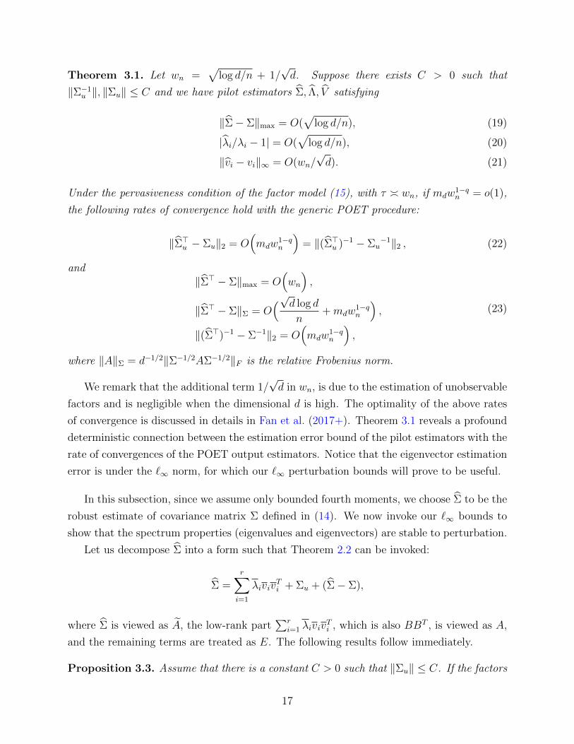
Theorem 3.1. Let wn =√

log d/n + 1/√d. Suppose there exists C > 0 such that

‖Σ−1u ‖, ‖Σu‖ ≤ C and we have pilot estimators Σ, Λ, V satisfying

‖Σ− Σ‖max = O(√

log d/n), (19)

|λi/λi − 1| = O(√

log d/n), (20)

‖vi − vi‖∞ = O(wn/√d). (21)

Under the pervasiveness condition of the factor model (15), with τ wn, if mdw1−qn = o(1),

the following rates of convergence hold with the generic POET procedure:

‖Σ>u − Σu‖2 = O(mdw

1−qn

)= ‖(Σ>u )−1 − Σu

−1‖2 , (22)

and‖Σ> − Σ‖max = O

(wn

),

‖Σ> − Σ‖Σ = O(√d log d

n+mdw

1−qn

),

‖(Σ>)−1 − Σ−1‖2 = O(mdw

1−qn

),

(23)

where ‖A‖Σ = d−1/2‖Σ−1/2AΣ−1/2‖F is the relative Frobenius norm.

We remark that the additional term 1/√d in wn, is due to the estimation of unobservable

factors and is negligible when the dimensional d is high. The optimality of the above rates

of convergence is discussed in details in Fan et al. (2017+). Theorem 3.1 reveals a profound

deterministic connection between the estimation error bound of the pilot estimators with the

rate of convergences of the POET output estimators. Notice that the eigenvector estimation

error is under the `∞ norm, for which our `∞ perturbation bounds will prove to be useful.

In this subsection, since we assume only bounded fourth moments, we choose Σ to be the

robust estimate of covariance matrix Σ defined in (14). We now invoke our `∞ bounds to

show that the spectrum properties (eigenvalues and eigenvectors) are stable to perturbation.

Let us decompose Σ into a form such that Theorem 2.2 can be invoked:

Σ =r∑i=1

λivivTi + Σu + (Σ− Σ),

where Σ is viewed as A, the low-rank part∑r

i=1 λivivTi , which is also BBT , is viewed as A,

and the remaining terms are treated as E. The following results follow immediately.

Proposition 3.3. Assume that there is a constant C > 0 such that ‖Σu‖ ≤ C. If the factors

17

are pervasive, then with probability greater than 1− d−1, we have (19) – (21) hold with λi, vi

as the leading eigenvalues/vectors of Σ for i ≤ r. In addition, (22) and (23) hold.

The inequality (19) follows directly from Proposition 3.1 under the assumption of

bounded fourth moments. It is also easily verifiable that (20), (21) follow from (19) by

Weyl’s inequality and Theorem 2.2 (noting that ‖Σu‖∞ ≤√d‖Σu‖). See Section 3.2 for

more details.

Note that in the case of sub-Gaussian variables, sample covariance matrix and its leading

eigenvalues/vectors will also serve the same purpose due to (12) and Theorem 2.2 as discussed

in Section 3.1.

We have seen that the `∞ perturbation bounds are useful in robust covariance estimation,

and particularly, they resolve a theoretical difficulty in the generic POET procedure for factor

model based covariance matrix estimation.

4 Simulations

4.1 Simulation: the perturbation result

In this subsection, we implement numerical simulations to verify the perturbation bound

in Theorem 2.2. We will show that the error behaves in the same way as indicated by our

theoretical bound.

In the experiments, we let the matrix size d run from 200 to 2000 by an increment

of 200. We fix the rank of A to be 3 (r = 3). To generate an incoherence low rank

matrix, we sample a d × d random matrix with iid standard normal variables, perform

singular value decomposition, and extract the first r right singular vectors v1, v2, . . . , vr. Let

V = (v1, . . . , vr) and D = diag(rγ, (r−1)γ, . . . , γ) where γ as before represents the eigengap.

Then, we set A = V DV T . By orthogonal invariance, vi is uniformly distributed on the unit

sphere Sd−1. It is not hard to see that with probability 1 − O(d−1), the coherence of V

µ(V ) = O(√

log d).

We consider two types of sparse perturbation matrices E: (a) construct a d × d matrix

E0 by randomly selecting s entries for each row, and sampling a uniform number in [0, L] for

each entry, and then symmetrize the perturbation matrix by setting E = (E0 + ET0 )/2; (b)

pick ρ ∈ (0, 1), L′ > 0, and let Eij = L′ρ|i−j|. Note that in (b) we have ‖E‖∞ ≤ 2L′/(1− ρ),

and thus we can choose suitable L′ and ρ to control the `∞ norm of E. This covariance

structure is common in cases where correlations between random variables depend on their

“distance” |i− j|, which usually arises from autoregressive models.

18

200 600 1000 1400 18000

0.05

0.1

0.15

0.2

0.25

0.3

0.35

0.4

d

err

5.5 6 6.5 7 7.5

−6.5

−5.6

−4.7

−3.8

−2.9

−2

−1.1

log d

log(err)

Figure 1: The left plot shows the perturbation error of eigenvectors against matrix size dranging from 200 to 2000, with different eigengap γ. The right plot shows log(err) againstlog(d). The slope is around −0.5. Blue lines represent γ = 10; red lines γ = 50; green linesγ = 100; and black lines γ = 500. We report the largest error over 100 runs.

The perturbation of eigenvectors is measured by the element-wise error:

err := max1≤i≤r

minηi∈±1

‖ηivi − vi‖∞,

where viri=1 are the eigenvectors of A = A+ E in the descending order.

To investigate how the error depends on γ and d, we generate E according to mechanism

(a) with s = 10, L = 3, and run simulations in different parameter configurations: (1) let

the matrix size d range from 200 to 2000, and choose the eigengap γ in 10, 50, 100, 500(Figure 1); (2) fix the product γ

√d to be one of 2000, 3000, 4000, 5000, and let the matrix

size d run from 200 to 2000 (Figure 2).

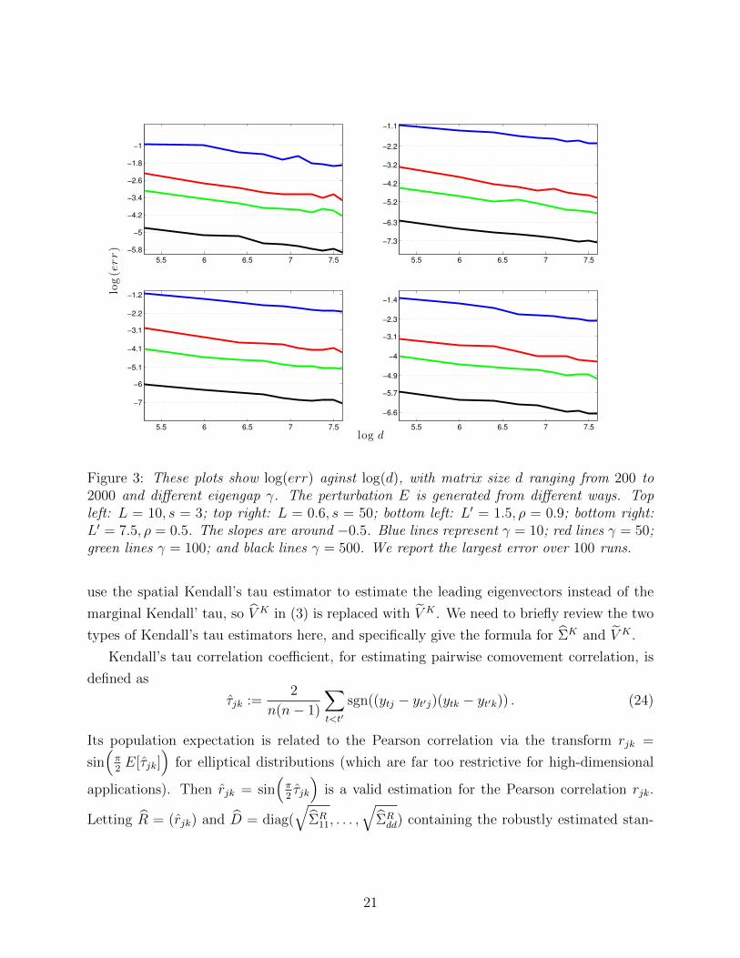
To find how the errors behave for E generated from different methods, we run simulations

as in (1) but generate E differently. We construct E through mechanism (a) with L =

10, s = 3 and L = 0.6, s = 50, and also through mechanism (b) with L′ = 1.5, ρ = 0.9 and

L′ = 7.5, ρ = 0.5 (Figure 3). The parameters are chosen such that ‖E‖∞ is about 30.

In Figure 1 – 3, we report the largest error based on 100 runs. Figure 1 shows that the

error decreases as d increases (the left plot); and moreover, the logarithm of the error is linear

in log(d), with a slope −0.5, that is, err ∝ 1/√d (the right plot). We can take the eigengap

19

200 600 1000 1400 18000

0.005

0.01

0.015

0.02

0.025

0.03

d

err

200 600 1000 1400 1800

5

15

25

35

45

55

65

75

d

err×

γ

√

d

Figure 2: The left plot shows the perturbation error of eigenvectors against matrix size dranging from 200 to 2000, when γ

√d is kept fixed, with different values. The right plot

shows the error multiplied by γ√d against d. Blue lines represent γ

√d = 2000; red lines

γ√d = 3000; green lines γ

√d = 4000; and black lines γ

√d = 5000. We report the largest

error over 100 runs.

γ into consideration and characterize the relationship in a more refined way. In Figure 2,

it is clear that err almost falls on the same horizontal line for different configurations of

d and γ, with γ√d fixed. The right panel clearly indicates that err × γ

√d is a constant,

and therefore err ∝ 1/(γ√d). In Figure 3, we find that the errors behave almost the same

regardless of how E is generated. These simulation results provide stark evidence supporting

the `∞ perturbation bound in Theorem 2.2.

4.2 Simulation: robust covariance esitmation

We consider the performance of the generic POET procedure in robust covariance estima-

tion in this subsection. Note that the procedure is flexible in employing any pilot estimators

Σ, Λ, V satisfying the conditions (19) – (21) respectively.

We implemented the robust procedure with four different initial trios: (1) the sample

covariance ΣS with its leading r eigenvalues and eigenvectors as ΛS and V S; (2) the Huber’s

robust estimator ΣR given in (14) and its top r eigen-structure estimators ΛR and V R; (3)

the marginal Kendall’s tau estimator ΣK with its corresponding ΛK and V K ; (4) lastly, we

20

5.5 6 6.5 7 7.5

−5.8

−5

−4.2

−3.4

−2.6

−1.8

−1

5.5 6 6.5 7 7.5

−7.3

−6.3

−5.2

−4.2

−3.2

−2.2

−1.1

5.5 6 6.5 7 7.5

−7

−6

−5.1

−4.1

−3.1

−2.2

−1.2

5.5 6 6.5 7 7.5

−6.6

−5.7

−4.9

−4

−3.1

−2.3

−1.4

log(err)

log d

Figure 3: These plots show log(err) aginst log(d), with matrix size d ranging from 200 to2000 and different eigengap γ. The perturbation E is generated from different ways. Topleft: L = 10, s = 3; top right: L = 0.6, s = 50; bottom left: L′ = 1.5, ρ = 0.9; bottom right:L′ = 7.5, ρ = 0.5. The slopes are around −0.5. Blue lines represent γ = 10; red lines γ = 50;green lines γ = 100; and black lines γ = 500. We report the largest error over 100 runs.

use the spatial Kendall’s tau estimator to estimate the leading eigenvectors instead of the

marginal Kendall’ tau, so V K in (3) is replaced with V K . We need to briefly review the two

types of Kendall’s tau estimators here, and specifically give the formula for ΣK and V K .

Kendall’s tau correlation coefficient, for estimating pairwise comovement correlation, is

defined as

τjk :=2

n(n− 1)

∑t<t′

sgn((ytj − yt′j)(ytk − yt′k)) . (24)

Its population expectation is related to the Pearson correlation via the transform rjk =

sin(π2E[τjk]

)for elliptical distributions (which are far too restrictive for high-dimensional

applications). Then rjk = sin(π2τjk

)is a valid estimation for the Pearson correlation rjk.

Letting R = (rjk) and D = diag(

√ΣR

11, . . . ,

√ΣRdd) containing the robustly estimated stan-

21

dard deviations, we define the marginal Kendall’s tau estimator as

ΣK = D R D . (25)

In the above construction of D, we still use the robust variance estimates from ΣR.

The spatial Kendall’s tau estimator is a second-order U-statstic, defined as

ΣK :=2

n(n− 1)

∑t<t′

(yt − yt′)(yt − yt′)T

‖yt − yt′‖22

. (26)

Then V S is constructed by the top r eigenvectors of ΣK . It has been shown by Fan et al.

(2017+) that under elliptical distribution, ΣK and its top r eigenvalues ΛK satisfy (19)

and (20) while V S suffices to conclude (21). Hence Method (4) indeed provides good initial

estimators if data are from elliptical distribution. However, since ΣK attains (19) for elliptical

distribution, by similar argument for deriving Proposition 3.3 based on our `∞ pertubation

bound, V K consisting of the leading eigenvectors of ΣK is also valid for the generic POET

procedure. For more details about the two types of Kendall’s tau, we refer the readers to

Fang et al. (1990); Choi and Marden (1998); Han and Liu (2014); Fan et al. (2017+) and

references therein.

In summary, Method (1) is designed for the case of sub-Gaussian data; Method (3)

and (4) work under the situation of elliptical distribution; while Method (2) is proposed in

this paper for the general heavy-tailed case with bounded fourth moments without further

distributional shape constraints.

We simulated n samples of (fTt , uTt )T from two settings: (a) a multivariate t-distribution

with covariance matrix diagIr, 5Id and various degrees of freedom (ν = 3 for very heavy

tail, ν = 5 for medium heavy tail and ν = ∞ for Gaussian tail), which is one example

of the elliptical distribution (Fang et al., 1990); (b) an element-wise iid one-dimensional t

distribution with the same covariance matrix and degrees of freedom ν = 3, 5 and ∞, which

is a non-elliptical heavy-tailed distribution.

Each row of coefficient matrix B is independently sampled from a standard normal dis-

tribution, so that with high probability, the pervasiveness condition holds with ‖B‖max =

O(√

log d). The data is then generated by yt = Bft + ut and the true population covariance

matrix is Σ = BBT + 5Id.

For d running from 200 to 900 and n = d/2, we calculated errors of the four robust

estimators in different norms. The tuning for α in minimization (14) is discussed more

throughly in Fan et al. (2017). For the thresholding parameter, we used τ = 2√

log d/n.

The estimation errors are gauged in the following norms: ‖Σ>u − Σu‖, ‖(Σ>)−1 − Σ−1‖ and

22

200 400 600 800

0.0

0.5

1.0

1.5

2.0

2.5

3.0

Spectral norm error of Sigma_u (Median)

p

erro

r ra

tio

200 400 600 800

0.0

0.5

1.0

1.5

2.0

2.5

3.0

Spectral norm error of Sigma_u (IQR)

p

erro

r ra

tio

200 400 600 800

0.0

0.5

1.0

1.5

2.0

2.5

3.0

Spectral norm error of inverse Sigma (Median)

p

erro

r ra

tio

200 400 600 800

0.0

0.5

1.0

1.5

2.0

2.5

3.0

Spectral norm error of inverse Sigma (IQR)

p

erro

r ra

tio

200 400 600 800

0.0

0.4

0.8

1.2

Relative Frobenius norm error of Sigma (Median)

p

erro

r ra

tio

200 400 600 800

0.0

0.4

0.8

1.2

Relative Frobenius norm error of Sigma (IQR)

p

erro

r ra

tio

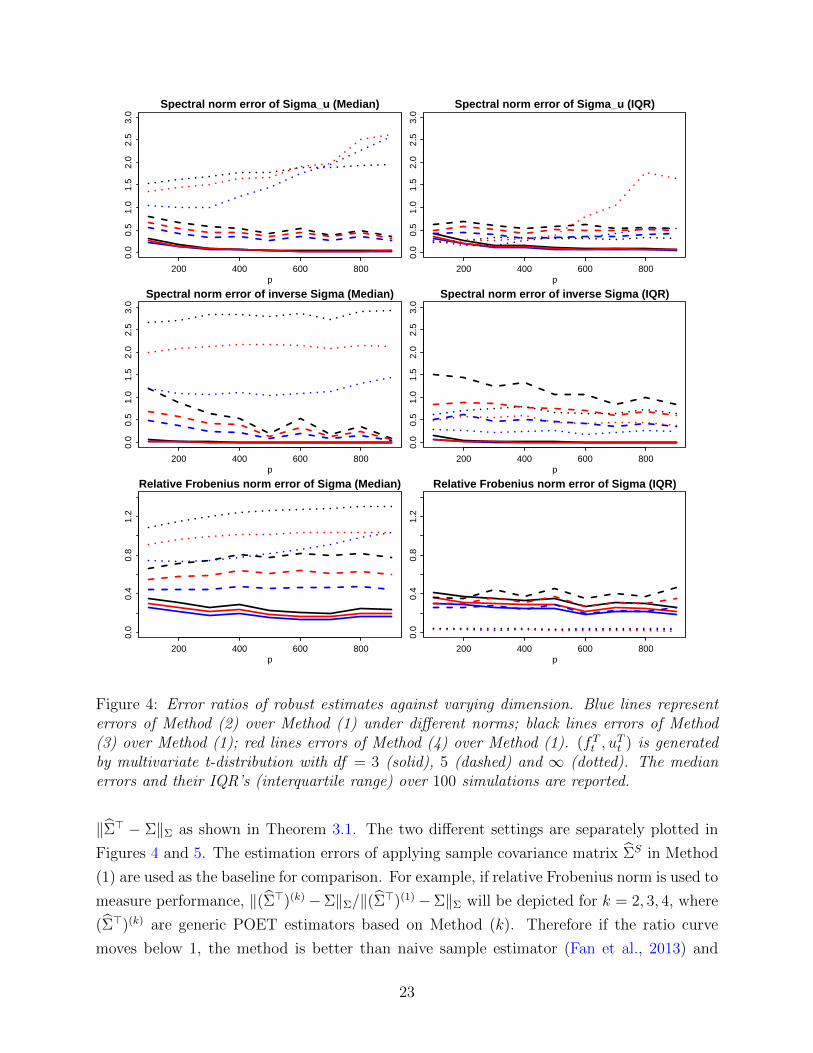
Figure 4: Error ratios of robust estimates against varying dimension. Blue lines representerrors of Method (2) over Method (1) under different norms; black lines errors of Method(3) over Method (1); red lines errors of Method (4) over Method (1). (fTt , u

Tt ) is generated

by multivariate t-distribution with df = 3 (solid), 5 (dashed) and ∞ (dotted). The medianerrors and their IQR’s (interquartile range) over 100 simulations are reported.

‖Σ> − Σ‖Σ as shown in Theorem 3.1. The two different settings are separately plotted in

Figures 4 and 5. The estimation errors of applying sample covariance matrix ΣS in Method

(1) are used as the baseline for comparison. For example, if relative Frobenius norm is used to

measure performance, ‖(Σ>)(k)−Σ‖Σ/‖(Σ>)(1)−Σ‖Σ will be depicted for k = 2, 3, 4, where

(Σ>)(k) are generic POET estimators based on Method (k). Therefore if the ratio curve

moves below 1, the method is better than naive sample estimator (Fan et al., 2013) and

23

vice versa. The more it gets below 1, the more robust the procedure is against heavy-tailed

randomness.

The first setting (Figure 4) represents a heavy-tailed elliptical distribution, where we

expect Methods (2), (3), (4) all outperform the POET estimator based on the sample co-

variance, i.e. Method (1), especially in the presence of extremely heavy tails (solid lines for

ν = 3). As expected, all three curves under various measures show error ratios visibly smaller

than 1. On the other hand, if data are indeed Gaussian (dotted line for ν =∞), Method (1)

has better behavior under most measures (error ratios are greater than 1). Nevertheless, our

robust Method (2) still performs comparably well with Method (1), whereas the median error

ratios for the two Kendall’s tau methods are much worse. In addition, the IQR (interquartile

range) plots reveal that Method (2) is indeed more stable than two Kendall’s tau Methods

(3) and (4). It is also noteworthy that Method (4), which leverages the advantage of spatial

Kendall’s tau, performs more robustly than Method (3), which solely base its estimation of

the eigen-structure on marginal Kendall’s tau.

The second setting (Figure 5) provides an example of non-elliptical distributed data. We

can see that the performance of the general robust Method (2) dominates the other three

methods, which verifies the benefit of robust estimation for a general heavy-tailed distribu-

tion. Note that Kendall’s tau methods do not apply to distributions outside the elliptical

family, excluding even the element-wise iid t distribution in this setting. Nonetheless, even

in the first setting where the data are indeed elliptical, with proper tuning, the proposed

robust method can still outperform Kendall’s tau by a clear margin.

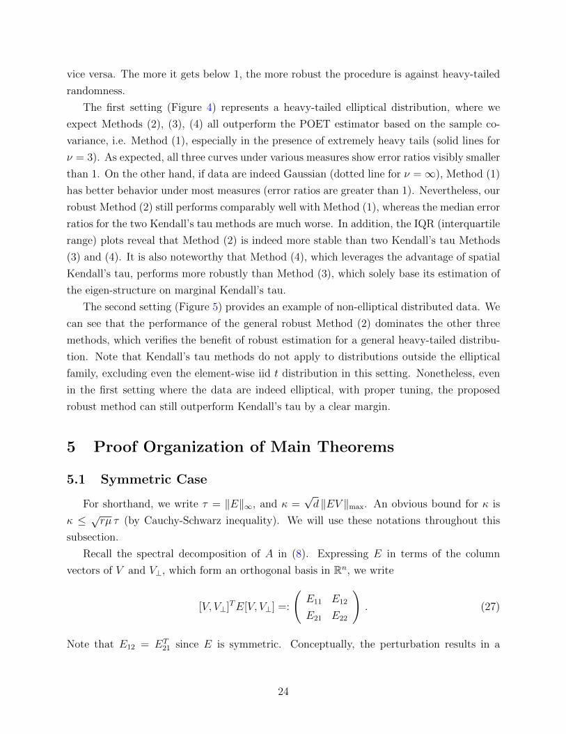
5 Proof Organization of Main Theorems

5.1 Symmetric Case

For shorthand, we write τ = ‖E‖∞, and κ =√d ‖EV ‖max. An obvious bound for κ is

κ ≤ √rµ τ (by Cauchy-Schwarz inequality). We will use these notations throughout this

subsection.

Recall the spectral decomposition of A in (8). Expressing E in terms of the column

vectors of V and V⊥, which form an orthogonal basis in Rn, we write

[V, V⊥]TE[V, V⊥] =:

(E11 E12

E21 E22

). (27)

Note that E12 = ET21 since E is symmetric. Conceptually, the perturbation results in a

24

200 400 600 800

0.0

0.5

1.0

1.5

2.0

2.5

3.0

Spectral norm error of Sigma_u (Median)

p

erro

r ra

tio

200 400 600 800

0.0

0.5

1.0

1.5

2.0

2.5

3.0

Spectral norm error of Sigma_u (IQR)

p

erro

r ra

tio

200 400 600 800

0.0

0.5

1.0

1.5

2.0

2.5

3.0

Spectral norm error of inverse Sigma (Median)

p

erro

r ra

tio

200 400 600 800

0.0

0.5

1.0

1.5

2.0

2.5

3.0

Spectral norm error of inverse Sigma (IQR)

p

erro

r ra

tio

200 400 600 800

0.0

0.4

0.8

1.2

Relative Frobenius norm error of Sigma (Median)

p

erro

r ra

tio

200 400 600 800

0.0

0.4

0.8

1.2

Relative Frobenius norm error of Sigma (IQR)

p

erro

r ra

tio

Figure 5: Error ratios of robust estimates against varying dimension. Blue lines representerrors of Method (2) over Method (1) under different norms; black lines errors of Method (3)over Method (1); red lines errors of Method (4) over Method (1). (fTt , u

Tt ) is generated by

element-wise iid t-distribution with df = 3 (solid), 5 (dashed) and ∞ (dotted). The medianerrors and their IQR’s (interquartile range) over 100 simulations are reported.

rotation of [V, V⊥], and we write a candidate orthogonal basis as follows:

V := (V + V⊥Q)(Ir +QTQ)−1/2, V ⊥ := (V⊥ − V QT )(Id−r +QQT )−1/2, (28)

where Q ∈ R(d−r)×r is to be determined. It is straightforward to check that [V , V ⊥] is

an orthogonal matrix. We will choose Q in a way such that (V , V ⊥)T A(V , V ⊥) is a block

25

diagonal matrix, i.e., VT

⊥AV = 0. Substituting (28) and simplifying the equation, we obtain

Q(Λ1 + E11)− (Λ2 + E22)Q = E21 −QE12Q. (29)

The approach of studying perturbation through a quadratic equation is known (see Stewart

(1990) for example). Yet, to the best of our knowledge, existing results study perturbation

under orthogonal-invariant norms (or unitary-invariant norms in the complex case), which

includes a family of matrix operator norms and Frobenius norm, but excludes the matrix

max-norm. The advantages of orthogonal-invariant norms are pronounced: such norms of a

symmetric matrix only depend on its eigenvalues regardless of eigenvectors; moreover, with

suitable normalization they are consistent in the sense ‖AB‖ ≤ ‖A‖ · ‖B‖. See Stewart

(1990) for a clear exposition.

The max-norm, however, does not possess these important properties. An imminent issue

is that it is not clear how to relate Q to V⊥Q, which will appear in (29) after expanding E

according to (27), and which we want to control. Our approach here is to study Q := V⊥Q

directly through a transformed quadratic equation, obtained by left multiplying V⊥ to (29).

Denote H = V⊥E21, Q = V⊥Q,L1 = Λ1 + E11, L2 = V⊥(Λ2 + E22)V T⊥ . If we can find an

appropriate matrix Q with Q = V⊥Q, and it satisfies the quadratic equation

QL1 − L2Q = H −QHTQ, (30)

then Q also satisfies the quadratic equation (29). This is because multiplying both sides of

(30) by V T⊥ yields (29), and thus any solution Q to (30) with the form Q = V⊥Q must result

in a solution Q to (29).

Once we have such Q (or equivalently Q), then (V , V ⊥)T A(V , V ⊥) is a block diagonal

matrix, and the span of column vectors of V is a candidate space of the span of first r

eigenvectors, namely spanv1, . . . , vr. We will verify the two spaces are identical in Lemma

5.3. Before stating that lemma, we first provide bounds on ‖Q‖max and ‖V − V ‖max.

Lemma 5.1. Suppose |λr| − ε > 4rµ(τ + 2rκ). Then, there exists a matrix Q ∈ R(d−r)×r

such that Q = V⊥Q ∈ Rd×r is a solution to the quadratic equation (30), and Q satisfies

‖Q‖max ≤ ω/√d. Moreover, if rω < 1/2, the matrix V defined in (28) satisfies

‖V − V ‖max ≤ 2√µωr/

√d . (31)

Here, ω is defined as ω = 8(1 + rµ)κ/(|λr| − ε).

The second claim of the lemma (i.e., the bound (31)) is relatively easy to prove once

the first claim (i.e., the bound on ‖Q‖max) is proved. To understand this, note that we can

26

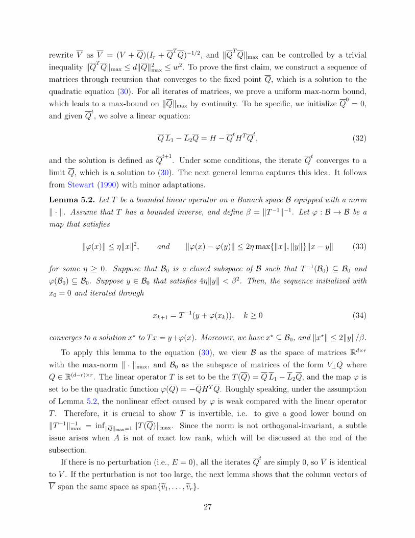
rewrite V as V = (V + Q)(Ir + QTQ)−1/2, and ‖QT

Q‖max can be controlled by a trivial

inequality ‖QTQ‖max ≤ d‖Q‖2

max ≤ w2. To prove the first claim, we construct a sequence of

matrices through recursion that converges to the fixed point Q, which is a solution to the

quadratic equation (30). For all iterates of matrices, we prove a uniform max-norm bound,

which leads to a max-bound on ‖Q‖max by continuity. To be specific, we initialize Q0

= 0,

and given Qt, we solve a linear equation:

QL1 − L2Q = H −QtHTQ

t, (32)

and the solution is defined as Qt+1

. Under some conditions, the iterate Qt

converges to a

limit Q, which is a solution to (30). The next general lemma captures this idea. It follows

from Stewart (1990) with minor adaptations.

Lemma 5.2. Let T be a bounded linear operator on a Banach space B equipped with a norm

‖ · ‖. Assume that T has a bounded inverse, and define β = ‖T−1‖−1. Let ϕ : B → B be a

map that satisfies

‖ϕ(x)‖ ≤ η‖x‖2, and ‖ϕ(x)− ϕ(y)‖ ≤ 2ηmax‖x‖, ‖y‖‖x− y‖ (33)

for some η ≥ 0. Suppose that B0 is a closed subspace of B such that T−1(B0) ⊆ B0 and

ϕ(B0) ⊆ B0. Suppose y ∈ B0 that satisfies 4η‖y‖ < β2. Then, the sequence initialized with

x0 = 0 and iterated through

xk+1 = T−1(y + ϕ(xk)), k ≥ 0 (34)

converges to a solution x? to Tx = y+ϕ(x). Moreover, we have x? ⊆ B0, and ‖x?‖ ≤ 2‖y‖/β.

To apply this lemma to the equation (30), we view B as the space of matrices Rd×r

with the max-norm ‖ · ‖max, and B0 as the subspace of matrices of the form V⊥Q where

Q ∈ R(d−r)×r. The linear operator T is set to be the T (Q) = QL1 − L2Q, and the map ϕ is

set to be the quadratic function ϕ(Q) = −QHTQ. Roughly speaking, under the assumption

of Lemma 5.2, the nonlinear effect caused by ϕ is weak compared with the linear operator

T . Therefore, it is crucial to show T is invertible, i.e. to give a good lower bound on

‖T−1‖−1max = inf‖Q‖max=1 ‖T (Q)‖max. Since the norm is not orthogonal-invariant, a subtle

issue arises when A is not of exact low rank, which will be discussed at the end of the

subsection.

If there is no perturbation (i.e., E = 0), all the iterates Qt

are simply 0, so V is identical

to V . If the perturbation is not too large, the next lemma shows that the column vectors of

V span the same space as spanv1, . . . , vr.

27

In other words, with a suitable orthogonal matrix R, the columns of V R are v1, . . . , vr.

Lemma 5.3. Suppose |λr| − ε > max3τ, 64(1 + rµ)r3/2µ1/2κ. Then, there exists an or-

thogonal matrix R ∈ Rr×r such that the column vectors of V R are v1, . . . , vr.

Proof of Theorem 2.1. It is easy to check that under the assumption of Theorem 2.1,

the conditions required in Lemma 5.1 and Lemma 5.3 are satisfied. Hence, the two lemmas

imply Theorem 2.1.

To study the perturbation of individual eigenvectors, we assume, in addition to the con-

dition on |λr|, that λ1, . . . , λr satisfy a uniform gap, (namely δ > ‖E‖2). This additional

assumption is necessary, because otherwise, the perturbation may lead to a change of rel-

ative order of eigenvalues, and we may be unable to match eigenvectors from the order of

eigenvalues. Suppose R ∈ Rr×r is an orthogonal matrix such that V R are eigenvectors of A.

Now, under the assumption of of Theorem 2.1, the column vectors of V and V R are identical

up to sign, so we can rewrite the difference V − V as

V − V = V (R− Ir) + (V − V ). (35)

We already provided a bound on ‖V − V ‖max in Lemma 5.1. By the triangular inequality,

we can derive a bound on ‖V ‖max. If we can prove a bound on ‖R − Ir‖max, it will finally

leads to a bound on ‖V − V ‖max. In order to do so, we use the Davis-Kahan theorem to

obtain an bound on 〈vi, vi〉 for all i ∈ [r]. This will lead to a max-norm bound on R − Ir(with the price of potentially increasing the bound by a factor of r). The details about the

proof of Theorem 2.2 are in the appendix.

We remark that, we assume conditions on |λr| − ε in Theorem 2.1 and Theorem 2.2,

which are only useful in cases where |λr| > ‖A−Ar‖∞. Ideally, we would like to have results

with assumptions only involving λr and λr+1, since Davis-Kahan theorem only requires a

gap in neighboring eigenvalues. Unfortunately, unlike orthogonal-invariant norms that only

depend on the eigenvalues of a matrix, the max-norm ‖ · ‖max is not orthogonal-invariant,

and thus it also depends on the eigenvectors of a matrix. For this reason, it is not clear

whether we could obtain a lower bound on ‖T−1‖−1max using only the eigenvalues λr and λr+1

so that we could apply Lemma 5.2. The analysis appears to be difficult if we do not have a

bound on ‖T−1‖−1max, considering that even in the analysis of linear equations, we also need

invertibility, condition numbers, etc.

28

5.2 Asymmetric Case

Let Ad, Ed be d1 + d2 square matrices defined as

Ad :=

(0 A

AT 0

), Ed :=

(0 E

ET 0

).

Also denote Ad := Ad + Ed. This augmentation of an asymmetric matrix into a symmetric

one is called Hermitian dilation. Here the superscript d means the Hermitian dilation. We

also use this notation to denote quantities corresponding to Ad and Ad.

An important observation is that(0 A

AT 0

)(ui

± vi

)= ±σi

(ui

± vi

).

From this identity, we know that Ad have nonzero eigenvalues ±σi where 1 ≤ i ≤ rank(A),

and its corresponding eigenvectors are (uTi ,± vTi )T . For a given r, we stack these (normalized)

eigenvectors with indices i ∈ [r] into a matrix V d ∈ R(d1+d2)×2r:

V d :=1√2

(U U

V −V

).

Through the augmented matrices, we can transfer eigenvector results for symmetric matrices

to singular vectors of asymmetric matrices. However, we cannot directly invoke the results

proved for symmetric matrices, due to an issue about the coherence of V d: when d1 and d2

are not comparable, the coherence µ(V d) can be very large even when µ(V ) and µ(U) are

bounded. To understand this, consider the case where r = 1, d1 d2, and all entries of U

are O(1/√d1), and all entries of V are O(1/

√d2). Then, the coherences µ(U) and µ(V ) are

O(1), but µ(V d) = O((d1 + d2)/d2) 1.

This unpleasant issue about the coherence, nevertheless, can be tackled if we consider a

different matrix norm. In order to deal with the different scales of d1 and d2, we define the

weighted max-norm for any matrix M with d1 + d2 rows as follows:

‖M‖w :=∥∥∥( √d1Id1 0

0√d2Id2

)M∥∥∥

max. (36)

In other words, we rescale the top d1 rows of M by a factor of√d1, and rescale the bottom

d2 rows by√d2. This weighted norm serves to balance the potential different scales of d1

and d2.

29

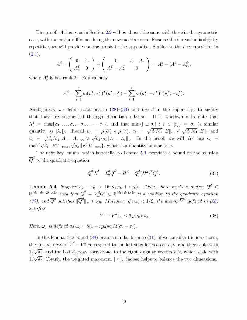
The proofs of theorems in Section 2.2 will be almost the same with those in the symmetric

case, with the major difference being the new matrix norm. Because the derivation is slightly

repetitive, we will provide concise proofs in the appendix . Similar to the decomposition in

(2.1),

Ad =

(0 Ar

ATr 0

)+

(0 A− Ar

AT − ATr 0

)=: Adr + (Ad − Adr),

where Adr is has rank 2r. Equivalently,

Adr =r∑i=1

σi(uTi , v

Ti )T (uTi , v

Ti )−

r∑i=1

σi(uTi ,−vTi )T (uTi ,−vTi ).

Analogously, we define notations in (28)–(30) and use d in the superscript to signify

that they are augmented through Hermitian dilation. It is worthwhile to note that

Λd1 = diagσ1, . . . , σr,−σr, . . . ,−σ1, and that min| ± σi| : i ∈ [r] = σr (a similar

quantity as |λr|). Recall µ0 = µ(U) ∨ µ(V ), τ0 =√d1/d2‖E‖∞ ∨

√d2/d1‖E‖1 and

ε0 =√d1/d2‖A − Ar‖∞ ∨

√d2/d1‖A − Ar‖1. In the proof, we will also use κ0 =

max√d1 ‖EV ‖max,

√d2 ‖ETU‖max, which is a quantity similar to κ.

The next key lemma, which is parallel to Lemma 5.1, provides a bound on the solution

Qd

to the quadratic equation

QdLd

1 − Ld

2Qd

= Hd −Qd(Hd)TQ

d. (37)

Lemma 5.4. Suppose σr − ε0 > 16rµ0(τ0 + rκ0). Then, there exists a matrix Qd ∈R(d1+d2−2r)×2r such that Q

d= V d

⊥Qd ∈ R(d1+d2)×2r is a solution to the quadratic equation

(37), and Qd

satisfies ‖Qd‖w ≤ ω0. Moreover, if rω0 < 1/2, the matrix Vd

defined in (28)

satisfies

‖V d − V d‖w ≤ 6√µ0 rω0 . (38)

Here, ω0 is defined as ω0 = 8(1 + rµ0)κ0/3(σr − ε0).

In this lemma, the bound (38) bears a similar form to (31): if we consider the max-norm,

the first d1 rows of Vd − V d correspond to the left singular vectors ui’s, and they scale with

1/√d1; and the last d2 rows correspond to the right singular vectors vi’s, which scale with

1/√d2. Clearly, the weighted max-norm ‖ · ‖w indeed helps to balance the two dimensions.

30

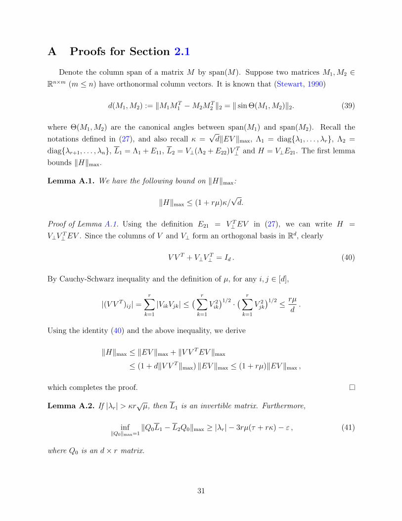
A Proofs for Section 2.1

Denote the column span of a matrix M by span(M). Suppose two matrices M1,M2 ∈Rn×m (m ≤ n) have orthonormal column vectors. It is known that (Stewart, 1990)

d(M1,M2) := ‖M1MT1 −M2M

T2 ‖2 = ‖ sin Θ(M1,M2)‖2. (39)

where Θ(M1,M2) are the canonical angles between span(M1) and span(M2). Recall the

notations defined in (27), and also recall κ =√d‖EV ‖max, Λ1 = diagλ1, . . . , λr, Λ2 =

diagλr+1, . . . , λn, L1 = Λ1 +E11, L2 = V⊥(Λ2 +E22)V T⊥ and H = V⊥E21. The first lemma

bounds ‖H‖max.

Lemma A.1. We have the following bound on ‖H‖max:

‖H‖max ≤ (1 + rµ)κ/√d.

Proof of Lemma A.1. Using the definition E21 = V T⊥ EV in (27), we can write H =

V⊥VT⊥ EV . Since the columns of V and V⊥ form an orthogonal basis in Rd, clearly

V V T + V⊥VT⊥ = Id . (40)

By Cauchy-Schwarz inequality and the definition of µ, for any i, j ∈ [d],

|(V V T )ij| =r∑

k=1

|VikVjk| ≤( r∑k=1

V 2ik

)1/2 ·( r∑k=1

V 2jk

)1/2 ≤ rµ

d.

Using the identity (40) and the above inequality, we derive

‖H‖max ≤ ‖EV ‖max + ‖V V TEV ‖max

≤ (1 + d‖V V T‖max) ‖EV ‖max ≤ (1 + rµ)‖EV ‖max ,

which completes the proof.

Lemma A.2. If |λr| > κr√µ, then L1 is an invertible matrix. Furthermore,

inf‖Q0‖max=1

‖Q0L1 − L2Q0‖max ≥ |λr| − 3rµ(τ + rκ)− ε , (41)

where Q0 is an d× r matrix.

31

Proof of Lemma A.2. Let Q0 be any d× r matrix with ‖Q0‖max = 1. Note

Q0L1 − L2Q0 = Q0Λ1 +Q0E11 − L2Q0.

We will derive upper bounds on Q0E11 and L2Q0, and a lower bound on Q0Λ1. Since

E11 = V TEV by definition, we expand Q0E11 and use a trivial inequality to derive

‖Q0E11‖max ≤ d ‖Q0VT‖max‖EV ‖max . (42)

By Cauchy-Schwarz inequality and the definition of µ in (3), for i, j ∈ [d],

|(Q0VT )ij| ≤

r∑k=1

|(Q0)ikVjk| ≤( r∑k=1

(Q0)2ik

)1/2 ( r∑k=1

V 2jk

)1/2 ≤√r ·√rµ

d,

Substituting ‖EV ‖max = κ/√d into (42), we obtain an upper bound:

‖Q0E11‖max ≤ κr√µ . (43)

To bound L2Q0 = (V⊥E22VT⊥ + (A− Ar))Q0, we use the identity (40) and write

V⊥E22VT⊥Q0 = V⊥V

T⊥ EV⊥V

T⊥Q0 = (Id − V V T )E(Id − V V T )Q0 .

Using two trivial inequalities ‖EQ0‖max ≤ ‖E‖∞‖Q0‖max = ‖E‖∞ and ‖V TQ0‖max ≤‖V T‖∞‖Q0‖max ≤

√d, we have

‖E(Id − V V T )Q0‖max ≤ ‖EQ0‖max + r‖EV ‖max‖V TQ0‖max

≤ ‖E‖∞ + r√d ‖EV ‖max = τ + rκ .

In the proof of Lemma A.1, we showed ‖V V T‖max ≤ rµ/d. Thus,

‖V⊥E22VT⊥Q0‖max ≤ (1 + d ‖V V T‖max) · ‖E(Id − V V T )Q0‖max ≤ (1 + rµ)(τ + rκ) .

Moreover, ‖(A− Ar)Q0‖max ≤ ‖A− Ar‖∞‖Q0‖max = ε. Combining the two bounds,

‖L2Q0‖max ≤ (1 + rµ)(τ + rκ) + ε. (44)

It is straightforward to obtain a lower bound on ‖Q0Λ1‖max: since there is an entry of Q0,

32

say (Q0)ij, that has an absolute value of 1, we have

‖Q0Λ1‖max ≥ |(Q0)ijλj| ≥ |λr|. (45)

To show L1 is invertible, we use (42) and (45) to obtain

‖Q0L1‖max ≥ ‖Q0Λ1‖max − ‖Q0E11‖max ≥ |λr| − κr√µ .

When |λr| − κr√µ > 0, L1 must have full rank, because otherwise we can choose an appro-

priate Q0 in the null space of LT

1 so that Q0L1 = 0, which is a contradiction. To prove the

second claim of the lemma, we combine the lower bound (45) with upper bounds (43) and

(44) to derive

‖Q0L1 − L2Q0‖max ≥ ‖Q0L1‖max − ‖Q0E11‖max − ‖L2Q0‖max

≥ |λr| − κr√µ− (1 + rµ)(τ + rκ)− ε

≥ |λr| − 3rµ(τ + rκ)− ε ,

which is exactly the desired inequality.

Next we prove Lemma 5.2. This lemma follows from Stewart (1990), with minor changes

that involves B0. We provide a proof for the sake of completeness.

Proof of Lemma 5.2. Let us write α = ‖y‖ for shorthand and recall β = ‖T−1‖−1. As

the first step, we show that the sequence xk∞k=0 is bounded. By construction in (34), we

bound ‖xk+1‖ using ‖xk‖:

‖xk+1‖ ≤ ‖T−1‖(‖y‖+ ‖ϕ(xk)‖) ≤α

β+η

β‖xk‖2.

We use this inequality to derive an upper bound on xk for all k. We define ξ0 = 0 and

ξk+1 =α

β+η

βξ2k, k ≥ 0,

then clearly ‖xk‖ ≤ ξk (which can be shown by induction). It is easy to check (by induction)

that the sequence ξk∞k=1 is increasing. Moreover, since 4αη < β2, the quadratic function

φ(ξ) =α

β+η

βξ2,

33

has two fixed points (namely solutions to φ(ξ) = ξ), and the smaller one satisfies

ξ? =2α

β +√β2 − 4ηα

<2α

β.

If ξk < ξ?, then ξk+1 = φ(ξk) ≤ φ(ξ?) = ξ?. Thus, by induction, all ξk are bounded by ξ?.

This implies ‖xk‖ ≤ ξ? < 2α/β. The next step is to show that the sequence xk converges.

Using the recursive definition (34) again, we derive

‖xk+1 − xk‖ ≤ ‖T−1‖‖ϕ(xk)− ϕ(xk−1)‖

≤ 2β−1ηmax‖xk‖, ‖xk−1‖‖xk − xk−1‖

≤ 4αη

β2‖xk − xk−1‖.

Since 4αη/β2 < 1, the sequence xk∞k=0 is a Cauchy sequence, and convergence is secured.

Let x? ∈ B be the limit. It is clear by assumption that xk ∈ B0 implies xk+1 ∈ B0, so x? ∈ B0

and ‖x?‖ ≤ 2α/β by continuity.

The final step is to show x? is a solution to Tx = y+φ(x). Because xk∞k=0 is bounded and

φ satisfies (33), the sequence φ(xk)∞k=0 converges to φ(x?) by continuity and compactness.

The linear operator T is also continuous, so we can take limits on both sides of Txk+1 =

y + φ(xk), we conclude that x? is a solution to Tx = y + φ(x).

With all the preparations, we are now ready to present the key lemma. As discussed in

Section 5, we set

B0 := Q ∈ Rd×r : Q = V⊥Q for some Q ∈ R(d−r)×r.

which is a subspace of B = Rd×r. Consider the matrix max-norm ‖ · ‖max in B.

Lemma A.3. Suppose |λr| − ε > 4rµ(τ + 2rκ). Then there exists a solution Q ∈ B0 to the

equation (30) with

‖Q‖max ≤8(1 + rµ)κ(|λr| − ε

)√d.

Proof of Lemma A.3. We will invoke Lemma 5.2 and apply it to the quadratic equation (30).

To do so, we first check the conditions required in Lemma 5.2.

Let the linear operator T be T Q = QL1 − L2Q. By Lemma A.2, T has a bounded

inverse, and β := ‖T −1‖−1max is bounded from below:

β ≥ |λr| − 3rµ(τ + rκ)− ε . (46)

34

Let us define ϕ by ϕ(Q) = QHTQ. To check the inequalities in (33), observe that

‖ϕ(Q)‖max ≤ rd‖Q‖max‖H‖max‖Q‖max ≤ (1 + rµ)κr√d ‖Q‖2

max

where we used Lemma A.1. We also observe

‖ϕ(Q1)− ϕ(Q2)‖max = ‖Q1HT (Q1 −Q2) + (Q1 −Q2)HTQ2‖max

≤ rd‖Q1‖max‖H‖max‖Q1 −Q2‖max + rd‖Q1 −Q2‖max‖H‖max‖Q2‖max

≤ 2(1 + rµ)κr√d max‖Q1‖max, ‖Q2‖max‖Q1 −Q2‖max.

Thus, if we set η = (1 + rµ)κr√d, then inequalities required in (33) are satisfied. For any

Q with Q = V⊥Q ∈ B0, obviously ϕ(Q) = V⊥QHTQ ∈ B0. To show T −1(Q) ∈ B0, let

Q0 = T −1(Q) and observe that

Q0L1 − L2Q0 = Q ∈ B0.

By definition, we know L2Q0 = V⊥(E22 + Λ2)V T⊥Q0 ∈ B0, so we deduce Q0L1 ∈ B0. Our

assumption implies |λr| > κr√µ, so by Lemma A.2, the matrix L1 is invertible, and thus

Q0 ∈ B0. The last condition we check is 4η‖H‖max < β2. By Lemma A.1 and (46), this is

true if

4(1 + rµ)2κ2r <[|λr| − 3rµ(τ + rκ)− ε

]2.

The above inequality holds when |λr| > 4rµ(V )(τ + 2rκ) + ε. Under this condition, we have,

by Lemma 5.2,

‖Q‖max ≤2(1 + rµ)κ(

|λr| − 3rµ(τ + rκ)− ε)√

d≤ 8(1 + rµ)κ

(|λr| − ε)√d,

where, the second inequality is due to 3rµ(τ + rκ) ≤ 3(|λr| − ε)/4.

The next lemma is a consequence of Lemma A.3. We define, as in Lemma 5.1, that

ω = 8(1 + rµ)κ/(|λr| − ε).

Lemma A.4. If rω2 < 1/2, then

‖(Ir +QTQ)−1/2 − Ir‖max ≤ rω2, ‖(Ir +Q

TQ)−1/2‖max ≤

3

2.

Proof of Lemma A.4. By the triangular inequality, the second inequality is immediate from

the first one. To prove the first inequality, suppose the spectral decomposition of QTQ is

QTQ = U ΣU

T, where Σ = diagλ1, . . . , λr where λ1 ≥ . . . ≥ λr, and U = [u1, u2, . . . , ur]

35

where u1, . . . , ur are orthonormal vectors in Rr. Since QTQ has nonnegative eigenvalues, we

have λr ≥ 0. Using these notations, we can rewrite the matrix as

(Ir +QTQ)−1/2 − Ir =

r∑i=1

((1 + λi)

−1/2 − 1)uiu

Ti .

Note that λ1 ≤ ‖QTQ‖ ≤ rd‖Q‖2

max ≤ rω2, which implies λ1 < 1/2. It is easy to check that

1+|x| ≥ (1+x)−1/2 ≥ 1−|x| whenever |x| < 1/2. From this fact, we know |(1+λi)−1/2−1| ≤

λi ≤ rω2. Using Cauchy-Schwarz inequality, we deduce that for any j, k ∈ [d],

∣∣[(Ir +QTQ)−1/2 − Ir]jk

∣∣ ≤ r∑i=1

∣∣(1 + λi)−1/2 − 1

∣∣ · ∣∣U jiUki

∣∣≤ rω2 ·

( r∑i=1

U2

ji

)1/2( r∑i=1

U2

ki

)1/2

≤ rω2.

This leads to the desired max-norm bound.

Proof of Lemma 5.1. The first claim of the lemma (the existence of Q and its max-norm

bound) follows directly from Lemma A.3. To prove the second claim, we split V − V into

two parts:

V − V = V((Ir +QTQ)−1/2 − Ir

)+ V⊥Q(Ir +QTQ)−1/2

= V(

(Ir +QTQ)−1/2 − Ir

)+Q(Ir +Q

TQ)−1/2, (47)

where we used identity V T⊥ V⊥ = Id−r. Note that rω < 1/2 implies rω2 = (rω)2/r < 1/(4r) <

1/2. Thus, we can use Lemma A.4 and derive

∥∥∥V ((Ir +QTQ)−1/2 − Ir

)∥∥∥max≤√r2µ

d‖(Ir +Q

TQ)−1/2 − Ir‖max ≤

õ

dr2ω2.

where we used Cauchy-Schwarz inequality. Using the above inequality and the bound on

‖Q‖max (namely, the first claim in the lemma),

‖V − V ‖max ≤√µ

dr2ω2 + r‖Q‖max‖(Ir +Q

TQ)−1/2‖max

≤ (√µω2r2 + 3ωr/2)/

√d.

36

Simplifying the bound using rω ≤ 1/2 and a trivial bound µ ≥ 1, we obtain (31).

Proof of Lemma 5.3. Using the identity in (39), it follows from Davis-Kahan sin Θ the-

orem (Davis and Kahan, 1970) and Weyl’s inequality that

d(V , V ) ≤ ‖E‖2

δr − ‖E‖2

,

when δr > ‖E‖2, where δr = |λr| − |λr+1|. Since λr+1 ≤ ‖A − Ar‖2 ≤ ε and ‖E‖2 ≤ τ , the

condition |λr| − ε > 3τ implies δr > 3‖E‖2. Hence, we have d(V , V ) < 1/2. Moreover,

d(V , V ) = ‖V V T − V V T‖2 ≤ ‖V (V − V )T‖2 + ‖(V − V )V T‖2

≤ 2‖V − V ‖2 ≤ 2√rd ‖V − V ‖max

≤ 4r3/2√µω,

where we used a trivial inequality ‖M‖2 ≤ ‖M‖F ≤√rd ‖M‖max for any M ∈ Rd×r. Under

the condition |λr| − ε > 64(1 + rµ)r3/2µ1/2κ, it is easy to check that 4r3/2√µω ≤ 1/2. Thus,

we obtain d(V , V ) < 1/2. By the triangular inequality,

d(V , V ) ≤ d(V , V ) + d(V , V ) < 1.

Since (V , V ⊥)T A(V , V ⊥) is a block diagonal matrix, span(V ) is the same as the subspace

spanned by r eigenvectors of A. We claim that span(V ) = span(v1, . . . , vr). Otherwise, there

exists an eigenvector u ∈ span(V ) whose associated eigenvalue is distinct from λ1, . . . , λr

(since δr > 3‖E‖2), and thus u is orthogonal to v1, . . . , vr. Therefore,

‖(V V T − V V T)u‖2 = ‖V V T

u‖2 = ‖u‖2.

This implies d(V , V ) ≥ 1, which is a contradiction.

Proof of Theorem 2.2. We split V −V into two parts—see (35). In the following, we first

obtain a bound on ‖R− Ir‖max, which then results in a bound on ‖V − V ‖max.

Under the assumption of the theorem, rω < 1/2, so

‖V ‖max ≤ ‖V − V ‖max + ‖V ‖max ≤ (2√µ rω)/

√d+√rµ/√d ≤ 2

√rµ/d . (48)

To bound ‖R− Ir‖max, we rewrite R as R = VTV R = V

TV . Expand V according to (28),

R = (Ir +QTQ)−1/2(V +Q)T V .

37

Let us make a few observations: (a) ‖QTV ‖max ≤

√d‖Q‖max ≤ ω by Cauchy-Schwarz

inequality; (b) ‖V TV ‖max ≤ 1 by Cauchy-Schwarz inequality again; and (c) ‖(Ir+QTQ)−1/2−

Ir‖max ≤ rω2 by Lemma A.4. Using these inequalities, we have

‖R− (V +Q)T V ‖max ≤ r‖(Ir +QTQ)−1/2 − Ir‖max ‖(V +Q)T V ‖max

≤ r2ω2(1 + ω) . (49)

Furthermore, by Davis-Kahn sin Θ theorem (Davis and Kahan, 1970) and Weyl’s inequality,

for any i ∈ [r],

sin θ(vi, vi) =√

1− 〈vi, vi〉2 ≤‖E‖2

δ − ‖E‖2

. (50)

when δ > ‖E‖2 (δ is defined in Theorem 2.2). This leads to the bound sin θ(vi, vi) ≤ 2‖E‖2/δ

(which is a simplified bound). This is because when δ ≥ 2‖E‖2, the bound is implied by

(50); when δ < 2‖E‖2, the bound trivially follows from sin θ(vi, vi) ≤ 1. We obtain, up to

sign, for i ≤ r, √1− 〈vi, vi〉 ≤

√1− 〈vi, vi〉2 ≤

2‖E‖2

δ. (51)

In other words, each diagonal entry of Ir−V T V , namely 1−〈vi, vi〉, is bounded by 4‖E‖22/δ

2.

Since viri=1 are orthonormal vectors, we have 1 − 〈vi, vi〉2 ≥∑

i′ 6=i〈vi, vi′〉2 ≥ 〈vi, vj〉2 for

any i 6= j, which leads to bounds on off-diagonal entries of V T V − Ir. We will combine the

two bounds. Note that when δ ≥ 2‖E‖2,

‖V T V − Ir‖max ≤ max4‖E‖2

2

δ2,2‖E‖2

δ

=

2‖E‖2

δ;

and when δ < 2‖E‖2, ‖V T V −Ir‖max is trivially bounded by 1 (up to sign), which is trivially

bounded by 2‖E‖2/δ. In either case, we deduce

‖V T V − Ir‖max ≤2‖E‖2

δ. (52)

Using the bounds in (49) and (52) and ‖QTV ‖max ≤ ω, we obtain

‖R− Ir‖max ≤ ‖R− (V +Q)T V ‖max + ‖V T V − Ir‖max + ‖QTV ‖max

≤ r2ω2(1 + ω) +2‖E‖2

δ+ ω .

38

We use the inequality rω < 1/2 to simplify the above bound:

‖R− Ir‖max ≤ r2ω2(1 + ω) + ω + 2‖E‖2/δ ≤ (1

2+

1

4+ 1)rω + 2‖E‖2/δ

≤ 2rω + 2‖E‖2/δ . (53)

We are now ready to bound ‖V − V ‖max. In (35), we use the bounds (48), (53), (31) to

obtain

‖V − V ‖max = ‖V (R− Ir) + (V − V )‖max ≤ r‖V ‖max‖R− Ir‖max + ‖V − V ‖max

≤ 2r√rµ/d (2rω + 2‖E‖2/δ) + 2r

√µω/√d

≤ (4r5/2µ1/2 + 2rµ1/2)ω√d

+4r3/2µ1/2‖E‖2

δ√d

≤ 48(1 + rµ)r5/2µ1/2κ

(|λr| − ε)√d

+4r3/2µ1/2‖E‖2

δ√d

.

Using a trivial inequality κ ≤ √rµ τ , the above bound leads to

‖V − V ‖max = O( r4µ2τ

(|λr| − ε)√d

+r3/2µ1/2‖E‖2

δ√d

).

B Proofs for Section 2.2

Recall the definitions of µ0, τ0, κ0 and ε0 in Section 5.2. Similar to the symmetric case,

we will use the following easily verifiable inequalities.

κ0 ≤√rµ0 τ0, ‖E‖2 ≤

(√d1/d2 ‖E‖∞ ·

√d2/d1 ‖E‖1

)1/2

≤ τ0. (54)

Lemma B.1. Parallel to Lemma A.1, we have

‖Hd‖w ≤ (1 + rµ0)κ0 ,

where κ0 =√d1 ‖EV ‖max ∨

√d2‖ETU‖max as defined.

Proof of Lemma B.1. Recall Hd = V d⊥(V d

⊥)TEdV d = EdV d − V d(V d)TEdV d. Note

39

V d(V d)T = diag(UUT , V V T ) and ‖UUT‖max ≤ rµ(U)/d1, ‖V V T‖max ≤ rµ(V )/d2. Thus,

‖Hd‖w ≤ ‖EdV d‖w + ‖V d(V d)TEdV d‖w≤ (1 + d1‖UUT‖max ∨ d2‖V V T‖max) ‖EdV d‖w ≤ (1 + rµ0)κ0 .

Lemma B.2. Parallel to Lemma A.2, if σr > 2κ0r√µ0, then L

d

1 is a non-degenerate matrix.

Furthermore, we have the following bound

inf‖Qd

0‖w=1‖Qd

0Ld

1 − Ld

2Qd0‖w ≥ σr − 4rµ0(τ0 + rκ0)− ε0 , (55)

where Qd0 ∈ R(d1+d2)×2r.

Proof of Lemma B.2. Following similar derivations with Lemma A.2, we have ‖Qd0E

d11‖w ≤

2κ0r√µ0, and for any matrix Qd

0 ∈ R(d1+d2)×2r with ‖Qd0‖w = 1,

‖Ld2Qd0‖w = ‖(Ad − Adr)Qd

0 + V d⊥(V d

⊥)TEdV d⊥(V d

⊥)TQd0‖w ≤ ε0 + (1 + rµ0)(τ0 + rκ0).

This can be checked by expressingQd0 as a block matrix and expand the matrix multiplication.

In particular, one can verify that (i) ‖(Ad − Adr)Qd0‖w ≤ ε0; (ii) For any matrix M with

d1 + d2 rows, ‖V d(V d)TM‖w ≤ rµ0‖M‖w; (iii) ‖EdQd0‖w ≤ τ0; (iv) ‖EdV d(V d)TQd

0‖w ≤ rκ0.

Moreover, ‖Qd0Λd

1‖w ≥ σr‖Qd0‖w ≥ σr. Thus,

inf‖Qd

0‖w=1‖Qd

0Ld

1 − Ld

2Qd0‖w ≥ σr − 4rµ0(τ0 + rκ0)− ε0 ,

which is the desired inequality in the lemma. In addition, Ld

1 is non-degenerate if σr >

2κ0r√µ0 > 0.

Lemma B.3. Parallel to Lemma A.3, there is a solution Qd ∈ B0 to the system (37) such

that if σr − ε0 > 16rµ0(τ0 + rκ0), then

‖Qd‖w ≤8(1 + rµ0)κ0

3(σr − ε0).

Proof of Lemma B.3. We again invoke Lemma 5.2. Let B be the space R(d1+d2)×2r equipped

with the weighted max-norm ‖ · ‖w. We also define B0 as a subspace of B consisting of

matrices of the form V d⊥Q

d where Qd has size (d1 + d2 − 2r) × 2r. Let the linear operator

T d be T dQd:= Q

dLd

1 − Ld

2Qd. First notice from Lemma B.2, T d is a linear operator with

40

bounded inverse, i.e., β := ‖(T d)−1‖−1w is bounded from below by

β ≥ σr − 4rµ0(τ0 + rκ0)− ε0 .

Let ϕ be a map given by ϕ(Qd) = Q

d(Hd)TQ

d. Note that Hd ∈ B. Using the (easily

verifiable) inequality

‖M1MT2 M3‖w ≤ 2r‖M1‖w‖MT

2 M3‖max ≤ 4r‖M1‖w‖M2‖w‖M3‖w ∀M1,M2,M3 ∈ B, (56)

we derive, by the bound on ‖Hd‖w (Lemma B.1), that

‖ϕ(Qd)‖w ≤ 4r‖Hd‖w‖Q

d‖2w ≤ 4r(1 + rµ0)κ0 ‖Q

d‖2w .

Moreover, using the inequality (56) and the bound on ‖Hd‖w (Lemma B.1),

‖ϕ(Qd

1)− ϕ(Qd

2)‖w ≤ 4r‖Qd

1‖w‖Hd‖w‖Qd

1 −Qd

2‖w + 4r‖Qd

1 −Qd

2‖w‖Hd‖w‖Qd

2‖w

≤ 8r(1 + rµ0)κ0 max‖Qd

1‖w, ‖Qd

2‖w‖Qd

1 −Qd

2‖w.

Thus, we can choose η = 4r(1 + rµ0)κ0, and the condition (33) in Lemma 5.2 is satisfied.

To ensure 4η‖Hd‖w < β2, it suffices to require (again by Lemma B.1),

16r(1 + rµ0)2κ20 <

[σr − 4rµ0(τ0 + rκ0)− ε0

]2.

It is easily checkable that the above inequality holds when σr− ε0 > 16rµ0(τ0 + rκ0). Under

this condition, by Lemma 5.2,

‖Qd‖w ≤2‖Hd‖w

β≤ 2(1 + rµ0)κ0

σr − 4rµ(τ0 + rκ0)− ε0

≤ 2(1 + rµ0)κ0

σr − ε0 − (σr − ε0)/4≤ 8(1 + rµ0)κ0

3(σr − ε0),

which completes the proof.

Proof of Lemma 5.4. The first claim of the lemma (existence of Qd

and its max-norm

bound) follows from Lemma B.3. To prove the second claim, we split Vd − V d into two

parts:

Vd − V d = V d

((I2r + (Q

d)T Q

d)−1/2 − I2r

)+Q

d(I2r + (Q

d)T Q

d)−1/2, (57)

Note κ0 ≤ τ0√rµ0 (see (54)). It can be checked that the condition σr− ε0 > 16rµ0(τ0 + rκ0)

implies rω0 < 1/3. Since ‖(Qd)TQ

d‖max ≤ 2ω20 and ‖(Qd

)TQd‖2 ≤ 2r‖(Qd

)TQd‖max ≤

41

4rω20 < 1/2, similar to Lemma A.4, we have

‖(I2r + (Qd)TQ

d)−1/2 − I2r‖max ≤ 4rω2

0, (58)

‖(I2r + (Qd)TQ

d)−1/2‖max ≤ 3/2.

This yields

‖V d − V d‖w = ‖V d(

(I2r + (Qd)TQ

d)−1/2 − I2r

)‖w + ‖Qd

(I2r + (Qd)TQ

d)−1/2‖w

≤√

2r2µ0 4rω20 + 2r · 3/2 · ‖Qd‖w ≤ 8

√µ0 ω

20r

2 + 3ω0r (59)

≤ 8√µ0 ω0r/3 + 3

√µ0 ω0r ≤ 6

√µ0 rω0. (60)

Lemma B.4. Suppose σr − ε0 > max16rµ0(τ0 + rκ0), 64r3/2µ1/20 (1 + rµ0)κ0. Then, there

exists an orthogonal matrix RV ∈ Rr×r (or RU) such that the column vectors of V RV (and

URU) are the top r right (and left) singular vectors of A.

Proof of Lemma B.4. Similar to the proof of Lemma 5.3, we will prove d(V , V ) < 1/2 and

d(V , V ) ≤ 1/2, which would then imply that V and V are the same only up to an orthogonal

transformation. The same is true for U and U , and we will leave out its proof.

By Weyl’s inequality for singular values (also known as Mirsky’s theorem (Mirsky, 1960)),

for any i, |σi − σi| ≤ ‖E‖. By Wedin’s perturbation bounds for singular vectors (Wedin,

1972),

d(V , V ) ≤ ‖E‖2

σr − ‖E‖2

.

Note that ‖E‖2 ≤ τ0 (see (54)) Under the assumption in the lemma, clearly σr − ε0 > 3τ0,

and we have d(V , V ) ≤ 1/2. Moreover, by Lemma 5.4, we have ‖V d − V d‖w ≤ 6rω0√µ0.

Note that each column vector of V d and Vd

are (d1 + d2)-dimensional. Looking at the last

d2 dimensions, we have ‖V − V ‖max ≤ 6rω0

õ0/d1.

d(V , V ) ≤ 2‖V − V ‖ ≤ 2√rd1‖V − V ‖max ≤ 12r3/2µ

1/20 ω0.

Under the assumption of the lemma, d(V , V ) ≤ 1/2. Therefore, we deduce d(V , V ) = 0, and

conclude that there exists an orthogonal matrix RV ∈ Rr×r such that V = V RV .

Proof of Theorem 2.3. Lemma 5.4, together with Lemma B.4, implies Theorem 2.3.

42

Proof of Theorem 2.4. Similar to the proof of Theorem 2.2, we first split the difference

V d − V d:

V d − V d = Vd(Rd − I2r) + (V

d − V d). (61)

To bound the first term, note that under our assumption, rω0 < 1/3 (derived in the proof

of Lemma 5.4), it is easy to check ‖V d‖w ≤ 3√rµ0. We rewrite the matrix Rd as

Rd = (I2r + (Qd)TQ

d)−1/2(V d +Q

d)T V d .

Notice that ‖(Qd)T V d‖max ≤

√2‖Qd‖w ≤

√2ω0, ‖(V d)TV d‖max ≤ 1 and

‖Rd − (V d +Qd)T V d‖max ≤ 2r‖(I2r + (Q

d)TQ

d)−1/2 − I2r‖max ‖(V d +Q

d)T V d‖max

≤ 8r2ω20(1 +

√2ω0) .

where we used (58). Following the same derivations as in the proof of Theorem 2.2, and using

the (easily verifiable) fact ‖Ed‖2 = ‖E‖2, we can bound ‖(V d)T V d − I2r‖max by 2‖E‖2/δ0.

Thus, using rω0 ≤ 1/3, under δ0 > 2‖E‖2, we have

‖Rd − I2r‖max ≤ ‖Rd − (V d +Qd)T V d‖max + ‖(V d)T V d − I2r‖max + ‖(Qd

)T V d‖max

≤ 8r2ω20(1 +

√2ω0) +

2‖E‖2

δ0

+√

2ω0 < 4√

2 rω0 +2‖E‖2

δ0

. (62)

Finally, in order to bound ‖V d − V d‖w, we use (60), (61) and (62), and derive

‖V d − V d‖w = ‖V d(Rd − I2r) + (V

d − V d)‖w ≤ 2r‖V d‖w‖Rd − I2r‖max + ‖V d − V d‖w

≤ 6r√rµ0

(4√

2 rω0 +2‖E‖2

δ0

)+ 6r√µ0 ω0 ≤

(40r5/2 ω0 + 12r3/2 ‖E‖2

δ0

)· √µ0

≤ 107r5/2µ1/20 (1 + rµ0)κ0

σr − ε0

+12r3/2µ

1/20 ‖E‖2

δ0

= O( r4µ2

0τ0

σr − ε0

+r3/2µ

1/20 ‖E‖2

δ0

).

This completes the proof.

C Proofs for Section 3

Proof of Proposition 3.2. Note first by Weyl’s inequality, |λi− λi| ≤ ‖Σu‖ ≤ C. So this

implies that λi = λi(BTB) d if and only if λi = λi(Σ) d for i ≤ r. And furthermore the

eigenvalues of BTB/d are distinct if and only if min1≤i 6=j≤r |λi(Σ)− λj(Σ)|/λj(Σ) > 0.

43

To prove the equivalency of bounded ‖B‖max and bounded coherence. We first prove

the necessary condition. Again from Weyl’s inequality, λi(Σ) ≤ C for i ≥ r + 1. If µ(V ) is

bounded, Σii must also be bounded, since Σii ≤∑r

j=1 v2ijλj(Σ) + λr+1(Σ) ≤ C(µ(V ) + 1).

Therefore ‖bi‖2 ≤ ‖bi‖2 + (Σu)ii = Σii implies ‖B‖max is bounded. Namely, the factors are

pervasive.

On the contrary, if pervasiveness holds, we need to prove that µ(V ) is bounded. Let

B = (b1, . . . , br). Obviously λi = ‖bi‖2 d and vi = bi/‖bi‖. Without loss of generality,

assume λi’s are decreasing. So ‖vi‖∞ ≤ ‖B‖max/‖bi‖ ≤ C/√d and µ(V ) ≤ C where V =

(v1, . . . , vr). By Theorem 2.2,

‖vi − vi‖∞ ≤ C‖Σu‖∞γ√d

,

where γ = minλi − λi+1 : 1 ≤ i ≤ r d with the convention λr+1 = 0. Hence, we have

‖vi‖∞ ≤ C/√d, which implies bounded coherence µ(V ).

References

Antoniadis, A. and Fan, J. (2001). Regularization of wavelet approximations. Journal

of the American Statistical Association 96.

Bai, J. (2003). Inferential theory for factor models of large dimensions. Econometrica 71

135–171.

Baik, J., Ben Arous, G. and Peche, S. (2005). Phase transition of the largest eigenvalue

for nonnull complex sample covariance matrices. Annals of Probability 1643–1697.

Bartholomew, D. J., Knott, M. and Moustaki, I. (2011). Latent variable models and

factor analysis: A unified approach, vol. 904. John Wiley & Sons.

Berthet, Q. and Rigollet, P. (2013). Optimal detection of sparse principal components

in high dimension. The Annals of Statistics 41 1780–1815.

Bickel, P. J. and Levina, E. (2008). Covariance regularization by thresholding. The

Annals of Statistics 2577–2604.

Biswas, P. and Ye, Y. (2004). Semidefinite programming for ad hoc wireless sensor network

localization. In Proceedings of the 3rd international symposium on Information processing

in sensor networks. ACM.

44

Borg, I. and Groenen, P. J. (2005). Modern multidimensional scaling: Theory and

applications. Springer Science & Business Media.

Cai, T. T. and Zhang, A. (2016). Rate-optimal perturbation bounds for singular subspaces

with applications to high-dimensional statistics. arXiv preprint arXiv:1605.00353 .

Candes, E. J., Li, X., Ma, Y. and Wright, J. (2011). Robust principal component

analysis? Journal of the ACM (JACM) 58 11.

Catoni, O. (2012). Challenging the empirical mean and empirical variance: a deviation

study. In Annales de l’Institut Henri Poincare, Probabilites et Statistiques, vol. 48. Institut

Henri Poincare.

Chamberlain, G. and Rothschild, M. (1982). Arbitrage, factor structure, and mean-

variance analysis on large asset markets.

Chandrasekaran, V., Sanghavi, S., Parrilo, P. A. and Willsky, A. S. (2011).

Rank-sparsity incoherence for matrix decomposition. SIAM Journal on Optimization 21

572–596.

Chen, Y. (2015). Incoherence-optimal matrix completion. IEEE Transactions on Informa-

tion Theory 61 2909–2923.

Choi, K. and Marden, J. (1998). A multivariate version of kendall’s τ . Journal of

Nonparametric Statistics 9 261–293.

Davis, C. and Kahan, W. M. (1970). The rotation of eigenvectors by a perturbation. iii.

SIAM Journal on Numerical Analysis 7 1–46.

De La Torre, F. and Black, M. J. (2003). A framework for robust subspace learning.

International Journal of Computer Vision 54 117–142.

Doherty, L., Pister, K. S. and El Ghaoui, L. (2001). Convex position estimation in

wireless sensor networks. In INFOCOM 2001. Twentieth Annual Joint Conference of the

IEEE Computer and Communications Societies. Proceedings. IEEE, vol. 3. IEEE.

Fama, E. F. and French, K. R. (1993). Common risk factors in the returns on stocks

and bonds. Journal of Financial Economics 33 3–56.

Fan, J., Fan, Y. and Lv, J. (2008). High dimensional covariance matrix estimation using

a factor model. Journal of Econometrics 147 186–197.

45

Fan, J., Li, Q. and Wang, Y. (2017). Robust estimation of high-dimensional mean

regression. Journal of Royal Statistical Society, Series B 79 247–265.

Fan, J., Liao, Y. and Mincheva, M. (2013). Large covariance estimation by thresholding

principal orthogonal complements. Journal of the Royal Statistical Society: Series B 75

1–44.

Fan, J., Liu, H. and Wang, W. (2017+). Large covariance estimation through elliptical

factor models. Annals of Statitistics to appear.

Fan, J., Wang, W. and Zhong, Y. (2017). Robust covariance estimation for approximate

factor models. Journal of Econometrics .

Fang, K.-T., Kotz, S. and Ng, K. W. (1990). Symmetric multivariate and related

distributions. Chapman and Hall.

Gupta, A. K., Varga, T. and Bodnar, T. (2013). Elliptically contoured models in

statistics and portfolio theory. Springer.

Han, F. and Liu, H. (2014). Scale-invariant sparse PCA on high-dimensional meta-elliptical

data. Journal of the American Statistical Association 109 275–287.

Hsu, D. and Sabato, S. (2014). Heavy-tailed regression with a generalized median-of-

means. In Proceedings of the 31st International Conference on Machine Learning (ICML-

14).

Hu, W., Tan, T., Wang, L. and Maybank, S. (2004). A survey on visual surveillance of

object motion and behaviors. Systems, Man, and Cybernetics, Part C: IEEE Transactions

on Applications and Reviews 34 334–352.

Huber, P. J. (1964). Robust estimation of a location parameter. The Annals of Mathe-

matical Statistics 35 73–101.

Johnstone, I. M. and Lu, A. Y. (2009). On consistency and sparsity for principal

components analysis in high dimensions. Journal of the American Statistical Association

104 682–693.

Jolliffe, I. (2002). Principal component analysis. Wiley Online Library.

Ma, Z. (2013). Sparse principal component analysis and iterative thresholding. The Annals

of Statistics 41 772–801.

46

Mirsky, L. (1960). Symmetric gauge functions and unitarily invariant norms. The quarterly

journal of mathematics 11 50–59.

Ng, A. Y., Jordan, M. I., Weiss, Y. et al. (2002). On spectral clustering: Analysis

and an algorithm. Advances in neural information processing systems 2 849–856.

Oliver, N. M., Rosario, B. and Pentland, A. P. (2000). A bayesian computer vision

system for modeling human interactions. IEEE Transactions on Pattern Analysis and

Machine Intelligence 22 831–843.

O’Rourke, S., Vu, V. and Wang, K. (2013). Random perturbation of low rank matrices:

Improving classical bounds. arXiv preprint arXiv:1311.2657 .

Paulsen, V. (2002). Completely bounded maps and operator algebras, vol. 78. Cambridge

University Press.

Rennie, J. D. and Srebro, N. (2005). Fast maximum margin matrix factorization for

collaborative prediction. In Proceedings of the 22nd international conference on Machine

learning. ACM.

Rohe, K., Chatterjee, S. and Yu, B. (2011). Spectral clustering and the high-

dimensional stochastic blockmodel. The Annals of Statistics 1878–1915.

Rothman, A. J., Levina, E. and Zhu, J. (2009). Generalized thresholding of large

covariance matrices. Journal of the American Statistical Association 104 177–186.

Stewart, G. W. (1990). Matrix perturbation theory .

Stock, J. and Watson, M. (2002). Forecasting using principal components from a large

number of predictors. Journal of the American Statistical Association 97 1167–1179.

Tropp, J. A. (2012). User-friendly tail bounds for sums of random matrices. Foundations

of Computational Mathematics 12 389–434.

Vershynin, R. (2010). Introduction to the non-asymptotic analysis of random matrices.

arXiv preprint arXiv:1011.3027 .

Vu, V. (2011). Singular vectors under random perturbation. Random Structures & Algo-

rithms 39 526–538.

Vu, V. Q. and Lei, J. (2012). Minimax rates of estimation for sparse pca in high dimensions.

arXiv preprint arXiv:1202.0786 .

47

Wang, W. and Fan, J. (2017+). Asymptotics of empirical eigen-structure for ultra-high

dimensional spiked covariance model. Annals of Statitistics to appear.

Wedin, P.-A. (1972). Perturbation bounds in connection with singular value decomposi-

tion. BIT Numerical Mathematics 12 99–111.

Yu, Y., Wang, T. and Samworth, R. J. (2015). A useful variant of the davis–kahan

theorem for statisticians. Biometrika 102 315–323.

Yuan, M., Ekici, A., Lu, Z. and Monteiro, R. (2007). Dimension reduction and

coefficient estimation in multivariate linear regression. Journal of the Royal Statistical

Society: Series B (Statistical Methodology) 69 329–346.

48