1 duke phd summer camp august 2007 outline motivation mutual consistency: ch model noisy...
TRANSCRIPT

August 2007 1Duke PhD Summer Camp
OutlineOutline
Motivation
Mutual Consistency: CH Model
Noisy Best-Response: QRE Model
Instant Convergence: EWA Learning

August 2007 2Duke PhD Summer Camp
Standard Assumptions in Standard Assumptions in Equilibrium AnalysisEquilibrium Analysis
Assumptions Nash Cognitive QRE EWAEquilbirum Hierarchy Learning
Solution Method
Strategic Thinking X X X X
Best Response X X XX
Mutual Consistency X
Instant Convergence X X X

August 2007 3Duke PhD Summer Camp
Example A: ExerciseExample A: Exercise
Consider matching pennies games in which the row player chooses between Top and Bottom and the column player simultaneously chooses between Left and Right, as shown below:
Left RightTop 80,40 40,80
Bottom 40,80 80,40
Left RightTop 320,40 40,80
Bottom 40,80 80,40
Left RightTop 44,40 40,80
Bottom 40,80 80,40
G1
G2

August 2007 4Duke PhD Summer Camp
Example A: ExerciseExample A: Exercise
Consider matching pennies games in which the row player chooses between Top and Bottom and the column player simultaneously chooses between Left and Right, as shown below:
Left RightTop 80,40 40,80
Bottom 40,80 80,40
Left RightTop 320,40 40,80
Bottom 40,80 80,40
Left RightTop 44,40 40,80
Bottom 40,80 80,40
G1
G2

August 2007 5Duke PhD Summer Camp
Example A: DataExample A: Data

August 2007 6Duke PhD Summer Camp
Example B: ExerciseExample B: Exercise
The two players choose “effort” levels simultaneously, and the payoff of each player is given by i = min (e1, e2) – c x ei
Efforts are integer from 110 to 170.

August 2007 7Duke PhD Summer Camp
Example B: ExerciseExample B: Exercise
The two players choose “effort” levels simultaneously, and the payoff of each player is given by i = min (e1, e2) – c x ei
Efforts are integer from 110 to 170.
C = 0.1 or 0.9.

August 2007 8Duke PhD Summer Camp
Example B: DataExample B: Data

August 2007 9Duke PhD Summer Camp
Motivation: CHMotivation: CH
Model heterogeneity explicitly (people are not equally smart)
Introduce the word surprise into the game theory’s dictionary (e.g., Next movie)
Generate new predictions (reconcile various treatment effects in lab data not predicted by standard theory)
Camerer, Ho, and Chong (QJE, 2004)

August 2007 10Duke PhD Summer Camp
Example 1: “zero-sum game”Example 1: “zero-sum game”
COLUMNL C R
T 0,0 10,-10 -5,5
ROW M -15,15 15,-15 25,-25
B 5,-5 -10,10 0,0
Messick(1965), Behavioral Science

August 2007 11Duke PhD Summer Camp
Nash Prediction: “zero-sum game”Nash Prediction: “zero-sum game”
Nash COLUMN Equilibrium
L C RT 0,0 10,-10 -5,5 0.40
ROW M -15,15 15,-15 25,-25 0.11
B 5,-5 -10,10 0,0 0.49Nash
Equilibrium 0.56 0.20 0.24

August 2007 12Duke PhD Summer Camp
CH Prediction: “zero-sum game”CH Prediction: “zero-sum game”
Nash CH ModelCOLUMN Equilibrium ( = 1.55)
L C RT 0,0 10,-10 -5,5 0.40 0.07
ROW M -15,15 15,-15 25,-25 0.11 0.40
B 5,-5 -10,10 0,0 0.49 0.53Nash
Equilibrium 0.56 0.20 0.24CH Model( = 1.55) 0.86 0.07 0.07

August 2007 13Duke PhD Summer Camp
Empirical Frequency: “zero-sum game”Empirical Frequency: “zero-sum game”
http://groups.haas.berkeley.edu/simulations/CH/
Nash CH Model EmpiricalCOLUMN Equilibrium ( = 1.55) Frequency
L C RT 0,0 10,-10 -5,5 0.40 0.07 0.13
ROW M -15,15 15,-15 25,-25 0.11 0.40 0.33
B 5,-5 -10,10 0,0 0.49 0.53 0.54Nash
Equilibrium 0.56 0.20 0.24CH Model( = 1.55) 0.86 0.07 0.07Empirical
Frequency 0.88 0.08 0.04

August 2007 14Duke PhD Summer Camp
The Cognitive Hierarchy (CH) ModelThe Cognitive Hierarchy (CH) Model
People are different and have different decision rules.
Modeling heterogeneity (i.e., distribution of types of players). Types of players are denoted by levels 0, 1, 2, 3,…,
Modeling decision rule of each type.

August 2007 15Duke PhD Summer Camp
Modeling Decision RuleModeling Decision Rule
Frequency of k-step is f(k)
Step 0 choose randomly
k-step thinkers know proportions f(0),...f(k-1)
Form beliefs and best-respond based on beliefs
Iterative and no need to solve a fixed point
gk (h) f (h)
f (h ' )h ' 1
K 1

August 2007 16Duke PhD Summer Camp
COLUMNL C R
T 0,0 10,-10 -5,5
ROW M -15,15 15,-15 25,-25
B 5,-5 -10,10 0,0
K's K+1's ROW COLLevel (K) Proportion Belief T M B L C R
0 0.212 1.00 0.33 0.33 0.33 0.33 0.33 0.33Aggregate 1.00 0.33 0.33 0.33 0.33 0.33 0.33
0 0.212 0.39 0.33 0.33 0.33 0.33 0.33 0.331 0.329 0.61 0 1 0 1 0 0
Aggregate 1.00 0.13 0.74 0.13 0.74 0.13 0.130 0.212 0.27 0.33 0.33 0.33 0.33 0.33 0.331 0.329 0.41 0 1 0 1 0 02 0.255 0.32 0 0 1 1 0 0
Aggregate 1.00 0.09 0.50 0.41 0.82 0.09 0.09
K Proportion, f(k)0 0.2121 0.3292 0.2553 0.132
>3 0.072
August 2007 17Duke PhD Summer Camp
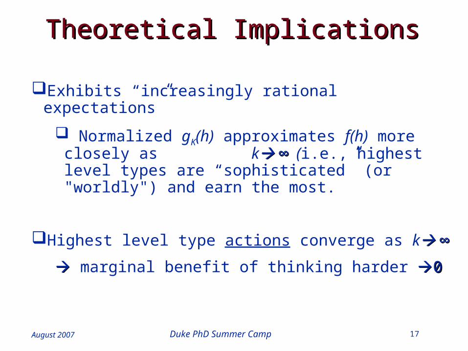
Theoretical ImplicationsTheoretical Implications
Exhibits “increasingly rational expectations”
Normalized gK(h) approximates f(h) more closely as k ∞ ∞ (i.e., highest level types are
“sophisticated” (or "worldly") and earn the most.
Highest level type actions converge as k ∞ ∞
marginal benefit of thinking harder 00

August 2007 18Duke PhD Summer Camp
Alternative SpecificationsAlternative Specifications
Overconfidence:
k-steps think others are all one step lower (k-1) (Stahl, GEB, 1995; Nagel, AER, 1995; Ho, Camerer and Weigelt, AER, 1998)
“Increasingly irrational expectations” as K ∞
Has some odd properties (e.g., cycles in entry games)
Self-conscious:
k-steps think there are other k-step thinkers
Similar to Quantal Response Equilibrium/Nash
Fits worse

August 2007 19Duke PhD Summer Camp
Modeling Heterogeneity, Modeling Heterogeneity, f(k)f(k)
A1:
sharp drop-off due to increasing difficulty in simulating others’ behaviors
A2: f(0) + f(1) = 2f(2)
kkf
kf
)1(
)(

August 2007 20Duke PhD Summer Camp
ImplicationsImplications
!)(
kekf
k A1 Poisson distribution with mean and variance =
A1,A2 Poisson, golden ratio Φ)

August 2007 21Duke PhD Summer Camp
Poisson DistributionPoisson Distribution
f(k) with mean step of thinking :!
)(k
ekfk
Poisson distributions for various
00.05
0.10.15
0.20.25
0.30.35
0.4
0 1 2 3 4 5 6
number of steps
fre
qu
en
cy

August 2007 22Duke PhD Summer Camp
Existence and Uniqueness:Existence and Uniqueness:CH SolutionCH Solution
Existence: There is always a CH solution in any game
Uniqueness: It is always unique

August 2007 23Duke PhD Summer Camp
Theoretical Properties of CH ModelTheoretical Properties of CH Model
Advantages over Nash equilibrium
Can “solve” multiplicity problem (picks one statistical distribution)
Sensible interpretation of mixed strategies (de facto purification)
Theory: τ∞ converges to Nash equilibrium in (weakly)
dominance solvable games

August 2007 24Duke PhD Summer Camp
Example 2: Entry gamesExample 2: Entry games
Market entry with many entrants:
Industry demand D (as % of # of players) is announced
Prefer to enter if expected %(entrants) < D;
Stay out if expected %(entrants) > D
All choose simultaneously
Experimental regularity in the 1st period: Consistent with Nash prediction, %(entrants) increases with D
“To a psychologist, it looks like magic”-- D. Kahneman ‘88
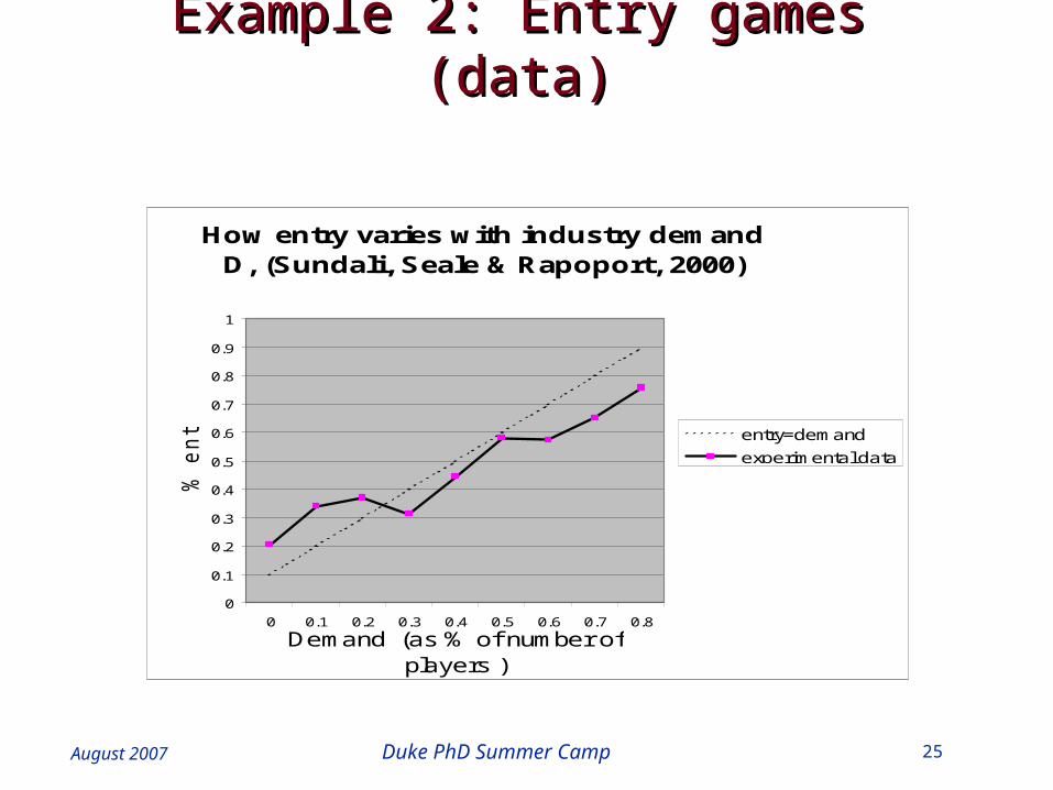
August 2007 25Duke PhD Summer Camp
How entry varies with industry demand D, (Sundali, Seale & Rapoport, 2000)
0
0.1
0.2
0.3
0.4
0.5
0.6
0.7
0.8
0.9
1
0 0.1 0.2 0.3 0.4 0.5 0.6 0.7 0.8
Demand (as % of number of players )
% e
ntr
y
entry=demand
experimental data
Example 2: Entry games (data)Example 2: Entry games (data)

August 2007 26Duke PhD Summer Camp
Behaviors of Level 0 and 1 Players ( =1.25)
Level 0
Level 1
% o
f E
nt r
y
Demand (as % of # of players)

August 2007 27Duke PhD Summer Camp
Behaviors of Level 0 and 1 Players (=1.25)
Level 0 + Level 1
% o
f E
nt r
y
Demand (as % of # of players)

August 2007 28Duke PhD Summer Camp
Behaviors of Level 2 Players(=1.25)
Level 2
Level 0 + Level 1
% o
f E
nt r
y
Demand (as % of # of players)

August 2007 29Duke PhD Summer Camp
Behaviors of Level 0, 1, and 2 Players ( =1.25)
Level 2
Level 0 +Level 1
Level 0 + Level 1 +Level 2
% o
f E
nt r
y
Demand (as % of # of players)

August 2007 30Duke PhD Summer Camp
How entry varies with demand (D), experimental data and thinking model
0
0.1
0.2
0.3
0.4
0.5
0.6
0.7
0.8
0.9
1
0 0.1 0.2 0.3 0.4 0.5 0.6 0.7 0.8
Demand (as % of # of players)
% e
ntr
y entry=demand
experimental data
CH Predictions in Entry Games CH Predictions in Entry Games (( = 1.25) = 1.25)

August 2007 31Duke PhD Summer Camp
HomeworkHomework
What value of can help to explain the data in Example A?
How does CH model explain the data in Example B?

August 2007 32Duke PhD Summer Camp
Empirical Frequency: “zero-sum game”Empirical Frequency: “zero-sum game”
COLUMN FrequencyL C R
T 0,0 10,-10 -5,5 0.125
ROW M -15,15 15,-15 25,-25 0.333
B 5,-5 -10,10 0,0 0.542Empirical
Frequency 0.875 0.083 0.042

August 2007 33Duke PhD Summer Camp
MLE EstimationMLE Estimation
Count LabelT 13 N1M 33 N2B 54 N3L 88 M1C 8 M2R 4 M3
321321 ))()(1()()())()(1()()()( 21212121MMMNNN qqqqppppLL

August 2007 34Duke PhD Summer Camp
Estimates of Mean Thinking Step Estimates of Mean Thinking Step
Table 1: Parameter Estimate for Cognitive Hierarchy Models
Data set Stahl & Cooper & Costa-GomesWilson (1995) Van Huyck et al. Mixed Entry
Game-specific Game 1 2.93 16.02 2.16 0.98 0.69Game 2 0.00 1.04 2.05 1.71 0.83Game 3 1.35 0.18 2.29 0.86 -Game 4 2.34 1.22 1.31 3.85 0.73Game 5 2.01 0.50 1.71 1.08 0.69Game 6 0.00 0.78 1.52 1.13Game 7 5.37 0.98 0.85 3.29Game 8 0.00 1.42 1.99 1.84Game 9 1.35 1.91 1.06Game 10 11.33 2.30 2.26Game 11 6.48 1.23 0.87Game 12 1.71 0.98 2.06Game 13 2.40 1.88Game 14 9.07Game 15 3.49Game 16 2.07Game 17 1.14Game 18 1.14Game 19 1.55Game 20 1.95Game 21 1.68Game 22 3.06Median 1.86 1.01 1.91 1.77 0.71
Common 1.54 0.80 1.69 1.48 0.73

August 2007 35Duke PhD Summer Camp
Table A1: 95% Confidence Interval for the Parameter Estimate of Cognitive Hierarchy Models
Data set
Lower Upper Lower Upper Lower Upper Lower Upper Lower UpperGame-specific Game 1 2.40 3.65 15.40 16.71 1.58 3.04 0.67 1.22 0.21 1.43Game 2 0.00 0.00 0.83 1.27 1.44 2.80 0.98 2.37 0.73 0.88Game 3 0.75 1.73 0.11 0.30 1.66 3.18 0.57 1.37 - -Game 4 2.34 2.45 1.01 1.48 0.91 1.84 2.65 4.26 0.56 1.09Game 5 1.61 2.45 0.36 0.67 1.22 2.30 0.70 1.62 0.26 1.58Game 6 0.00 0.00 0.64 0.94 0.89 2.26 0.87 1.77Game 7 5.20 5.62 0.75 1.23 0.40 1.41 2.45 3.85Game 8 0.00 0.00 1.16 1.72 1.48 2.67 1.21 2.09Game 9 1.06 1.69 1.28 2.68 0.62 1.64Game 10 11.29 11.37 1.67 3.06 1.34 3.58Game 11 5.81 7.56 0.75 1.85 0.64 1.23Game 12 1.49 2.02 0.55 1.46 1.40 2.35Game 13 1.75 3.16 1.64 2.15Game 14 6.61 10.84Game 15 2.46 5.25Game 16 1.45 2.64Game 17 0.82 1.52Game 18 0.78 1.60Game 19 1.00 2.15Game 20 1.28 2.59Game 21 0.95 2.21Game 22 1.70 3.63
Common 1.39 1.67 0.74 0.87 1.53 2.13 1.30 1.78 0.42 1.07
Stahl &Wilson (1995)
Cooper &Van Huyck
Costa-Gomeset al. Mixed Entry
CH Model: CI of Parameter Estimates

August 2007 36Duke PhD Summer Camp
Table 2: Model Fit (Log Likelihood LL and Mean-squared Deviation MSD)
Stahl & Cooper & Costa-GomesData set Wilson (1995) Van Huyck et al. Mixed Entry
Cognitive Hierarchy (Game-specific ) LL -721 -1690 -540 -824 -150MSD 0.0074 0.0079 0.0034 0.0097 0.0004Cognitive Hierarchy (Common )LL -918 -1743 -560 -872 -150MSD 0.0327 0.0136 0.0100 0.0179 0.0005
Cognitive Hierarchy (Common )LL -941 -1929 -599 -884 -153MSD 0.0425 0.0328 0.0257 0.0216 0.0034
Nash Equilibrium 1 LL -3657 -10921 -3684 -1641 -154MSD 0.0882 0.2040 0.1367 0.0521 0.0049
Note 1: The Nash Equilibrium result is derived by allowing a non-zero mass of 0.0001 on non-equilibrium strategies.
Within-dataset Forecasting
Cross-dataset Forecasting
Nash versus CH Model: LL and MSD

August 2007 37Duke PhD Summer Camp
Figure 2a: Predicted Frequencies of Cognitive Hierarchy Models
for Matrix Games (common )
y = 0.868x + 0.0499
R2 = 0.8203
0
0.1
0.2
0.3
0.4
0.5
0.6
0.7
0.8
0.9
1
0 0.1 0.2 0.3 0.4 0.5 0.6 0.7 0.8 0.9 1
Empirical Frequency
Pre
dic
ted
Fre
qu
en
cy
CH Model: Theory vs. Data(Mixed Games)

August 2007 38Duke PhD Summer Camp
Figure 3a: Predicted Frequencies of Nash Equilibrium for Matrix Games
y = 0.8273x + 0.0652
R2 = 0.3187
0
0.1
0.2
0.3
0.4
0.5
0.6
0.7
0.8
0.9
1
0 0.1 0.2 0.3 0.4 0.5 0.6 0.7 0.8 0.9 1
Empirical Frequency
Pre
dic
ted
Fre
qu
en
cy
Nash: Theory vs. Data (Mixed Games)

August 2007 39Duke PhD Summer Camp
Nash vs. CH (Mixed Games)

August 2007 40Duke PhD Summer Camp
Figure 2b: Predicted Frequencies of Cognitive Hierarchy Models
for Entry and Mixed Games (common )
y = 0.8785x + 0.0419
R2 = 0.8027
0
0.1
0.2
0.3
0.4
0.5
0.6
0.7
0.8
0.9
1
0 0.1 0.2 0.3 0.4 0.5 0.6 0.7 0.8 0.9 1
Empirical Frequency
Pre
dic
ted
Fre
qu
en
cy
CH Model: Theory vs. Data(Entry and Mixed Games)

August 2007 41Duke PhD Summer Camp
Figure 3b: Predicted Frequencies of Nash Equilibrium for Entry and Mixed Games
y = 0.707x + 0.1011
R2 = 0.4873
0
0.1
0.2
0.3
0.4
0.5
0.6
0.7
0.8
0.9
1
0 0.1 0.2 0.3 0.4 0.5 0.6 0.7 0.8 0.9 1
Empirical Frequency
Pre
dic
ted
Fre
qu
en
cy
Nash: Theory vs. Data (Entry and Mixed Games)

August 2007 42Duke PhD Summer Camp
CH vs. Nash (Entry and Mixed Games)

August 2007 43Duke PhD Summer Camp
Economic ValueEconomic Value
Evaluate models based on their value-added rather than statistical fit (Camerer and Ho, 2000)
Treat models like consultants
If players were to hire Mr. Nash and Ms. CH as consultants and listen to their advice (i.e., use the model to forecast what others will do and best-respond), would they have made a higher payoff?
A measure of disequilibrium

August 2007 44Duke PhD Summer Camp
Nash versus CH Model: Economic Value

August 2007 45Duke PhD Summer Camp
Example 3Example 3: P: P-Beauty Contest-Beauty Contest
n players
Every player simultaneously chooses a number from 0
to 100
Compute the group average
Define Target Number to be 0.7 times the group
average
The winner is the player whose number is the closet to
the Target Number
The prize to the winner is US$20

August 2007 46Duke PhD Summer Camp
Results in various Results in various pp-BC games -BC games

August 2007 47Duke PhD Summer Camp
Results in various Results in various pp-BC games -BC games
Subject Pool Group Size Sample Size Mean Error (Nash)
Error (CH)
CEOs 20 20 37.9 -37.9 -0.1 1.080 year olds 33 33 37.0 -37.0 -0.1 1.1Economics PhDs 16 16 27.4 -27.4 0.0 2.3Portfolio Managers 26 26 24.3 -24.3 0.1 2.8Game Theorists 27-54 136 19.1 -19.1 0.0 3.7

August 2007 48Duke PhD Summer Camp
SummarySummary
CH Model:
Discrete thinking steps
Frequency Poisson distributed
One-shot games
Fits better than Nash and adds more economic value
Explains “magic” of entry games
Sensible interpretation of mixed strategies
Can “solve” multiplicity problem
Initial conditions for learning

August 2007 49Duke PhD Summer Camp
OutlineOutline
Motivation
Mutual Consistency: CH Model
Noisy Best-Response: QRE Model
Instant Convergence: EWA Learning