1

Copyright © Cengage Learning. All rights reserved.

Differentiation2

Basic Differentiation Rules and Rates of Change

Copyright © Cengage Learning. All rights reserved.

2.2

4

Find the derivative of a function using the Constant Rule.

Find the derivative of a function using the Power Rule.

Find the derivative of a function using the Constant Multiple Rule.

Objectives

5

Find the derivative of a function using the Sum and Difference Rules.

Find the derivatives of the sine function and of the cosine function.

Use derivatives to find rates of change.

Objectives

6

The Constant Rule

7

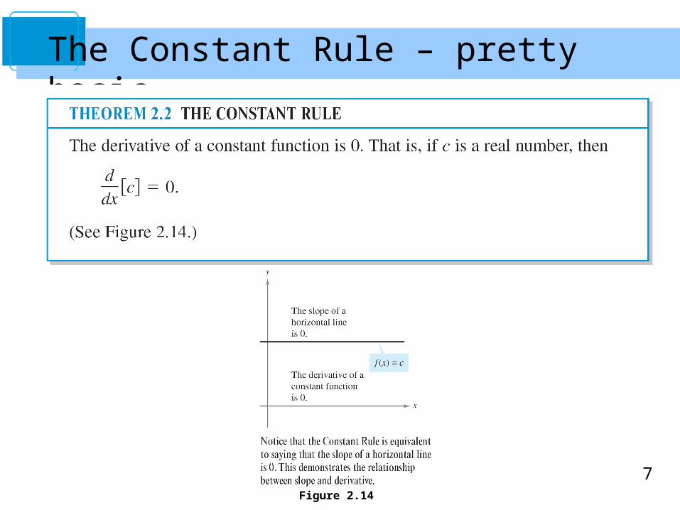
The Constant Rule – pretty basic

Figure 2.14

8

Example 1 – Using the Constant Rule

9

The Power Rule

10

The Power Rule

Before proving the next rule, it is important to review the procedure for expanding a binomial.

The general binomial expansion for a positive integer n is

This binomial expansion is used in proving a special case of the Power Rule.

MIDDLE TERMS!Need to do these, not just assume you already know what they come out to be!

11

The Power Rule

The Power Rule implemented:1) Bring the power out front as a coefficient2) Reduce the power by one

12

When using the Power Rule, the case for which n = 1 is best thought of as a separate differentiation rule. That is,

This rule is consistent with the fact that the slope of the line y = x is 1,as shown in Figure 2.15.

Figure 2.15

The Power Rule

13

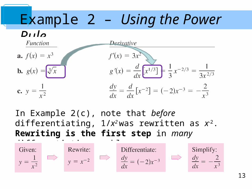
Example 2 – Using the Power Rule

In Example 2(c), note that before differentiating, 1/x2 was rewritten as x-2. Rewriting is the first step in many differentiation problems.

14

The Constant Multiple Rule

15

The Constant Multiple Rule

16

Example 5 – Using the Constant Multiple Rule

The Constant Multiple Rule implemented:1) Move the coefficient out front of the derivative2) Implement the Power Rule as before3) Simplify

17

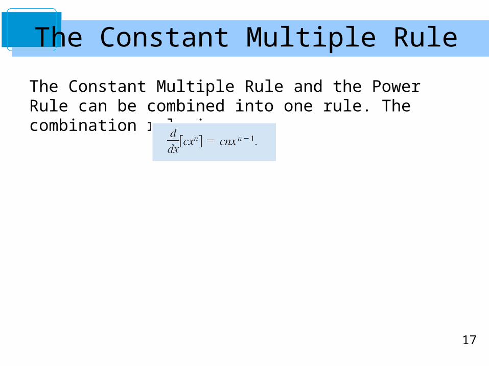
The Constant Multiple Rule and the Power Rule can be combined into one rule. The combination rule is

The Constant Multiple Rule

18

The Sum and Difference Rules

19

The Sum and Difference Rules

20

Example 7 – Using the Sum and Difference Rules

The Sum or Difference Rules implemented:1) Differentiate each term separately2) Implement the rule as before

21

Derivatives of the Sine and Cosine Functions

22

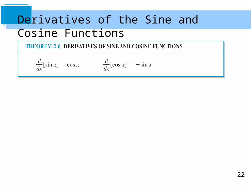
Derivatives of the Sine and Cosine Functions

23

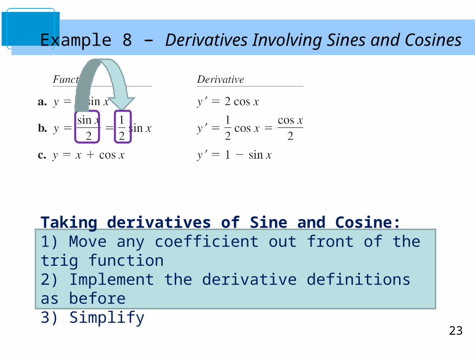
Example 8 – Derivatives Involving Sines and Cosines

Taking derivatives of Sine and Cosine:1) Move any coefficient out front of the trig function2) Implement the derivative definitions as before3) Simplify

24

Assignment 12

• Read: pp107-114

• Watch: PP2.2

• Do: pp 115-118/1-29odd, 34,36,37,45,50, 59-65odd,99-101,107,112 (29 problems)

• Due: Thursday

25

Rates of Change

26

You have seen how the derivative is used to determine slope.

The derivative can also be used to determine the rate of change of one variable with respect to another.

Applications involving rates of change occur in a wide variety of fields.

A few examples are population growth rates, production rates, water flow rates, velocity, and acceleration.

Rates of Change

27

A common use for rate of change is to describe the motion of an object moving in a straight line.

In such problems, it is customary to use either a horizontal or a vertical line with a designated origin to represent the line of motion.

On such lines, movement to the right (or upward) is considered to be in the positive direction, and movement to the left (or downward) is considered to be in the negative direction.

Rates of Change

28

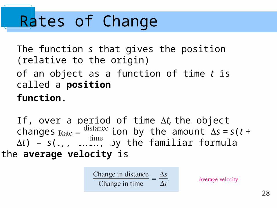
The function s that gives the position (relative to the origin)

of an object as a function of time t is called a position

function.

If, over a period of time t, the object changes its position by the amount s = s(t + t) – s(t), then, by the familiar formula

the average velocity is

Rates of Change

29

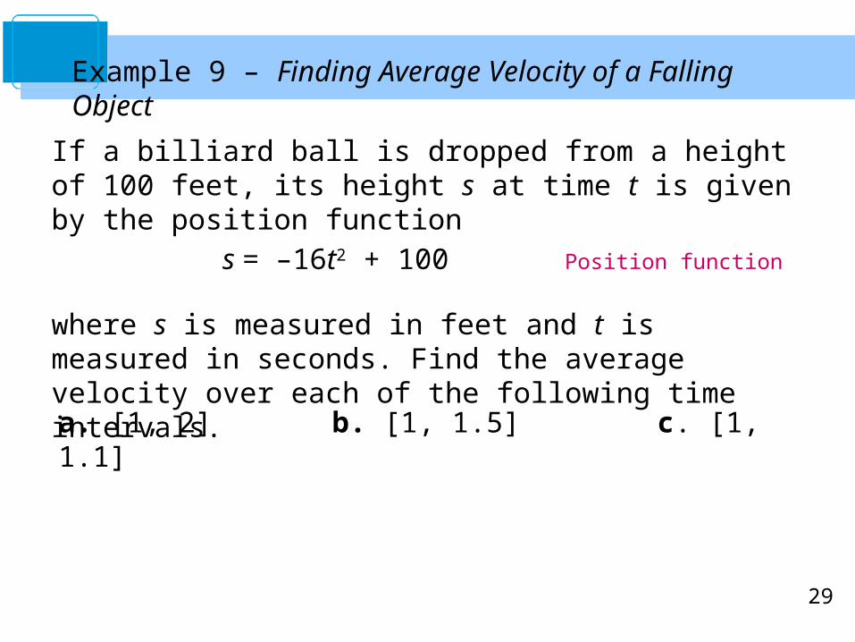
If a billiard ball is dropped from a height of 100 feet, its height s at time t is given by the position function

s = –16t2 + 100 Position function

where s is measured in feet and t is measured in seconds. Find the average velocity over each of the following time intervals.

Example 9 – Finding Average Velocity of a Falling Object

a. [1, 2] b. [1, 1.5] c. [1, 1.1]

30

For the interval [1, 2], the object falls from a height of

s(1) = –16(1)2 + 100 = 84 feet to a height of

s(2) = –16(2)2 + 100 = 36 feet.

Example 9(a) – Solution

The average velocity is

31

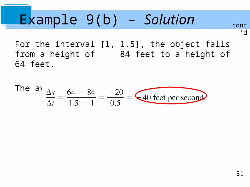
Example 9(b) – Solution

For the interval [1, 1.5], the object falls from a height of 84 feet to a height of 64 feet.

The average velocity is

cont’d

32

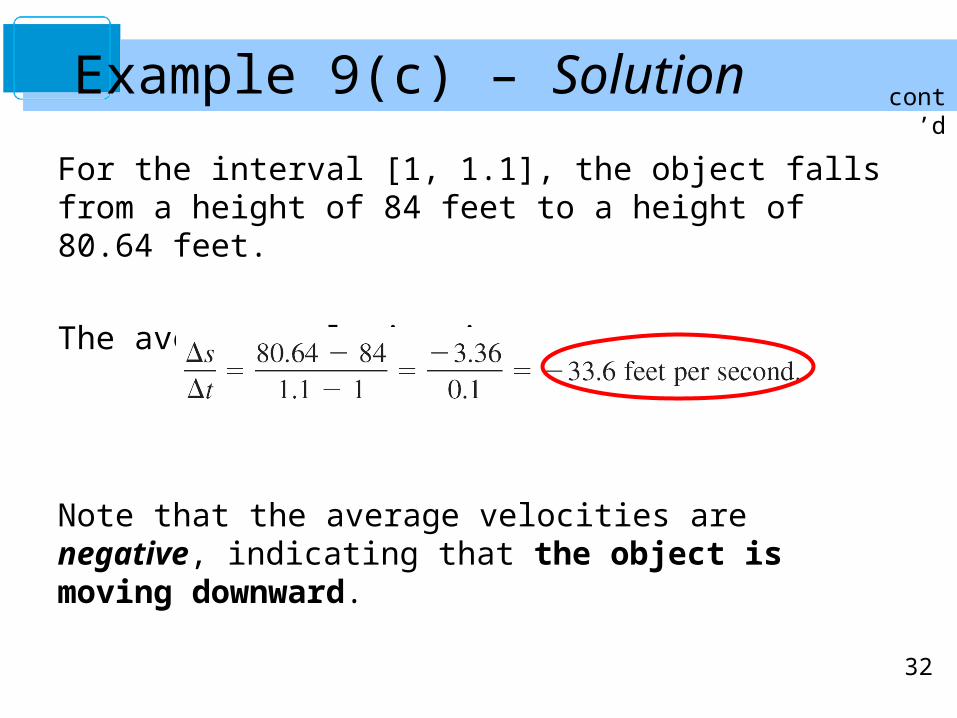
For the interval [1, 1.1], the object falls from a height of 84 feet to a height of 80.64 feet.

The average velocity is

Note that the average velocities are negative, indicating that the object is moving downward.

Example 9(c) – Solution cont’d

33

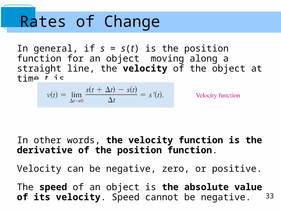
In general, if s = s(t) is the position function for an object moving along a straight line, the velocity of the object at time t is

In other words, the velocity function is the derivative of the position function.

Velocity can be negative, zero, or positive.

The speed of an object is the absolute value of its velocity. Speed cannot be negative.

Rates of Change

34

The position of a free-falling object (neglecting air resistance) under the influence of gravity can be represented by the equation

where s0 is the initial height of the object, v0 is the initial velocity of the object, and g is the acceleration due to gravity.

On Earth, the value of g is approximately –32 feet per second per second or –9.8 meters per second per second.

Rates of Change

In general, this book uses US rather than

metric units

35

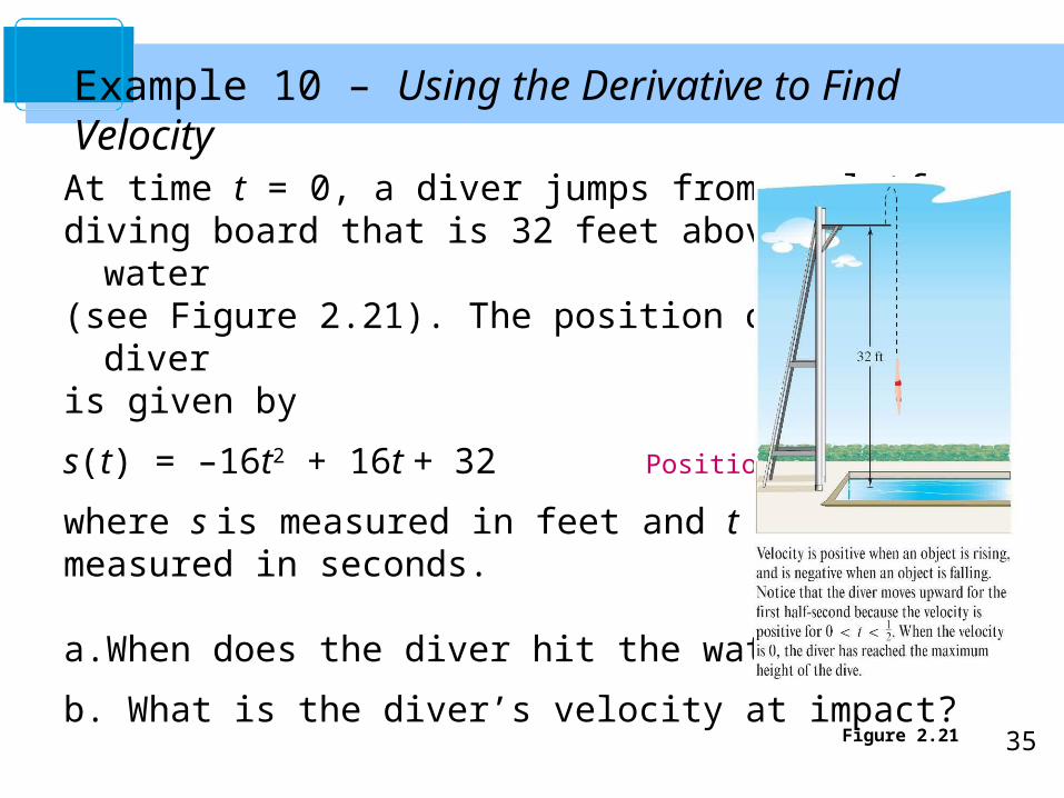
Example 10 – Using the Derivative to Find Velocity

At time t = 0, a diver jumps from a platform diving board that is 32 feet above the water(see Figure 2.21). The position of the diveris given by

s(t) = –16t2 + 16t + 32 Position function

where s is measured in feet and t is measured in seconds.

a. When does the diver hit the water?

b. What is the diver’s velocity at impact?

Figure 2.21

36

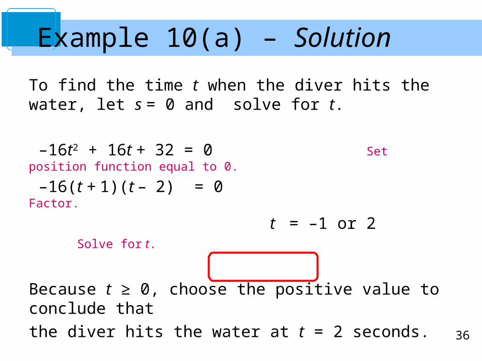
Example 10(a) – Solution

To find the time t when the diver hits the water, let s = 0 and solve for t.

–16t2 + 16t + 32 = 0 Set position function equal to 0.

–16(t + 1)(t – 2) = 0 Factor.

t = –1 or 2 Solve for t.

Because t ≥ 0, choose the positive value to conclude that

the diver hits the water at t = 2 seconds.

37

Example 10(b) – Solution

The velocity at time t is given by the derivative

s(t) = –32t + 16.

So, the velocity at time is t = 2 is s(2) = –32(2) + 16

= –48 feet per second.

cont’d

38

Assignment 12

• Read: pp107-114

• Watch: PP2.2

• Do: pp 115-118/1-29odd, 34,36,37,45,50, 59-65odd,99-101,107,112 (29 problems)

• Due: Thursday