1

Classifying by Multiple Features: Naive Bayes

• e : The example (instance) to be classified– word occurrence, document

• c : a class, among all possible classes C – word sense, document category

• f : Feature – context word, document word

2

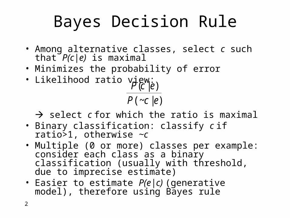
Bayes Decision Rule

• Among alternative classes, select c such that P(c|e) is maximal

• Minimizes the probability of error• Likelihood ratio view:

select c for which the ratio is maximal• Binary classification: classify c if ratio>1, otherwise ~c• Multiple (0 or more) classes per example: consider each

class as a binary classification (usually with threshold, due to imprecise estimate)

• Easier to estimate P(e|c) (generative model), therefore using Bayes rule

)|(~)|(ecP

ecP

3

Conditional Probability and Bayes Rule

]Pr[

]Pr[]Pr[]Pr[

Rule Bayes

],Pr[]Pr[

]Pr[

]Pr[]Pr[

]Pr[

]Pr[]Pr[

happend has event given event ofy Probabilit

:yProbabilit lConditiona

B

AABBA

BABA

A

BAAB

B

BABA

BA

A B

A

B

4

Bayes and Independence Assumption

Bayes )(~)|~(

)()|()|(~

)|(cPceP

cPcePecP

ecP

assumption

ceindependen

)(~)(

)|~(

)|(

cPcP

cfP

cfP

ef

ef

Posterior Prior

5

Log-Likelihood Ratio• Computational convenience – avoid underflow

• Estimate probabilities from training corpus, by (smoothed) count ratios

• : the “entailment score” of f for c

• Working with this ratio indicates explicitly feature “weight” within the score, compared to– log P(f|c) itself is large for frequent f’s, regardless of discrimination

• Was applied to many classification tasks

)|~()|(

logcfP

cfP

ef CP

CP

cfP

cfP

ecP

ecPcscore

)(~

)(log

)|~(

)|(log

)|(~

)|(log)(

ef

CPcfPcscore )(log)|(log)(

6

Word Sense Disambiguationby Naïve Bayes

• Each ambiguous word w is a classification problem

• e : The example (instance) to be classified– An occurrence of the ambiguous word

• c : a class, among all possible classes C – A word sense, among all listed senses

• f : Feature – A context word or phrase, in near or broad

context, possibly within a syntactic relationship

7

Estimating Probabilities• Assume a sense labeled training corpus• Apply some smoothing to avoid zero counts:

• freq(c) – sum of all context positions• Context features (words) that tend to occur mostly with a

specific sense, and not with the others, contribute high values to its accumulative score

• Gale, Church and Yarowsky (1992) report 90% accuracy for 6 ambiguous nouns– Combining weaker evidence from broad context, vs. stronger

collocations used in decisions based on single feature

)(

)()(

)(

),()|(

wfreq

cfreqcP

cfreq

cffreqcfP

8

Examples for Significant Features

• Senses of drug (Gale et al. 1992):

‘medication’ prices, prescription, patent,

increase, consumer,

pharmaceutical

‘illegal substance’

abuse, paraphernalia, illicit,

alcohol, cocaine, traffickers

9

Text Categorization

• A document is labeled by its “major” categories (event type, entities, geography) – typically the major topics discussed in the document

• “Controlled vocabulary” – categories taken from a canonical pre-defined list (hierarchy/taxonomy) – to be distinguished from free-text terms– Used for consistent searching and browsing

• Document features: terms, weighted by frequency (mostly), position, …

• Category: typically represented by triggering rules or feature weights, applied to test documents

10

Types of Text Categorization Tasks

• Topical (multiple classes per document)– Broad: finance, politics, sports– Detailed: investment, sale, merger

• Genre: news, contract, movie review, editorial• Authorship (style-based): individual, gender• Attitude: positive, negative• Relevance

– Generic: spam, junk mail, pornography– Personal interests

• Applications: filtering, routing, search, browsing

11

Categorization Approaches (with Some Industrial Perspective)

• Manual labeling by authors/editors– Still the most common approach in practice

• Supervised automatic classification– Manual encoding of classification rules (instead of

training) – requires special expertise

– Supervised machine learning• Training documents are labeled manually (cost!)

• Requires (somewhat) less expertise

– Combined• Users can modify the learned “logic” (rules, weights)

• “Bootstrapping” of classification “logic” (no labeling)

12

Features in Text Categorization

• Feature space dimensionality is very high – each word, possibly word-combinations– Vs. many other learning tasks

• Only a relatively small number of features is usually relevant for each category

• Learning methods need to be robust for very high dimensionality, and avoid overfitting for coincidental feature-category correlations in training

• Apparent advantage to methods that combine evidence from many features, vs. methods that consider relatively few (e.g. decision trees/lists)

13

Text Categorization with Naïve Bayes

• Consider each category independently as a class c (for the multiple class setting)– Example e – document– Feature f – word or term

– Classify c if score(c)>θ • Typically a specifically tuned threshold for each class, due to

inaccuracy of the probabilistic estimate of P(e|c) with given training statistics and independence assumption,

• .. but a biased probability estimate for c may still correlate well with the classification decision

ef CP

CP

cfP

cfP

ecP

ecPcscore

)(~

)(log

)|~(

)|(log

)|(~

)|(log)(

14

Two Feature Models

• 1st Model: Multivariate binomial– One binary feature f corresponds to each word in the

(corpus) lexicon

– f is true in a document (triggered for the example) if the word appears in it, and false otherwise

– Parameter estimation:

– Notice that in classification each word in the document contributes its “weight” once, regardless of its frequency

• But according to the model, words that do not appear in the document take part in the classification too (~f)

)|(1)|(~ )(

),()|( cfPcfP

cdoc_count

cfdoc_countcfP

15

2nd Model: Multinomial

• One multinomial feature f corresponds to each position in the document

• Feature value is the identity of the word at the corresponding position; possible values are all words in the lexicon – For brevity, we use f to denote both the feature and its value

• Parameter estimation:

• Notice that in classification each word contributes its “weight” multiplied by its frequency in the document

)(

),()|(

ccountposiotion_

cfountposition_ccfP

16

Some Observations on the Models• Multinomial model has an advantage of taking into

account word frequency in the document, but:– According to experience in Information Retrieval (IR),

multiplying a word “weight” by its frequency yields inflated impact of frequent words in a document (multiple occurrences of a word are dependent). E.g., a word weight is multiplied in IR by the log of its frequency in the document

– Considering frequency boosts the misleading effect of word ambiguity: a word correlated with the category might appear frequently in a document but under an alternate sense; the binomial model “emphasizes” accumulating weight from multiple words, and its unlikely that several words that are correlated with the category will occur together under alternate senses.

• Both models do not distinguish well between words that really trigger the category vs. words that refer to other frequently correlated topics

Relevant language behavior should be analyzed when choosing a model; some aspects are beyond basic model

17

Naïve Bayes Properties• Very simple and efficient

– Training: one pass over the corpus to count feature-class co-occurrences

– Classification: linear in the number of “active” features in the example

• Not the best model but often not much worse than more complex models– Often a useful quick solution; good baseline for advanced models

• Works well when classification is triggered by multiple, roughly equally indicative, features

• Relatively robust to irrelevant features, which typically cancel each other– But feature selection often helps (needed)– Somewhat sensitive to features that correspond to different but

correlated classes (whether such classes are defined or not)

18

Feature Selection• Goal: enable the learning method to focus on

the most informative features, either globally or per class, reducing the noise introduced by irrelevant features

• Most simple criterion: feature frequency– For some categorization results: 10 times feature

space reduction with no accuracy loss; 100 times reduction with small loss

– Typical filters: at most 1-3 docs, 1-5 occurrences

19

Feature Selection (cont.)• More complicated selection scores based on

feature-category co-occurrence frequency– Computed per-category, possibly obtaining a global

score by sum/weighted average/max

– The same data as in actual classification by Bayes, but used to decide whether to ignore the feature altogether

a b

c d

f

~f

C ~C

20

Example Selection Score Functions

• Mutual information for ci,tk:

Recall MI (for variables):

• Information gain:

• Odds ratio:

• Galavotti et al. (2000)

}{ }{ )()(

),(log),();(

x y ypxp

yxpyxpYXI

21

Linear Classifiers

• Linear classifier:

• Classify e to c if

• s(f,e) (the variable): “strength” of f in e (e.g. some function of f’s frequency in e)

• w(f,c) (the coefficient): the weight of f in the vector representing c

• Two dimensional case:

• Compare s and w with unsupervised association

ef

cfwefscescore ),(),(),(

),( cescore

ybxa+ +

+

+

+

- -- - -

22

Naive Bayes as a Linear Classifier

• In Naive Bayes - classify e for c if:

•

0)(~

)(log

)|~()|(

log)|(~

)|(log

ef CPCP

cfPcfP

ecPecP

)|~()|(

log

otherwise 0

1),(

)|~()|(

log),(

cfPcfP

efefs

cfPcfP

cfw

23

Perceptron (Winnow): Non-Parametric Mistake-Driven Learning of w(f,c)

For a category c:

foreach f initialize w(f,c) (uniformly/randomly)

do until no_errors or time_limit

foreach (e in training)

compute score(e,c)

if (score(e,c) <= teta && pos(e)) #false

negative

do foreach (f in e)

w(f,c) += alpha (*= alpha)

if (score(e,c) >= teta && neg(e)) #false

positive

do foreach (f in e)

w(f,c) -= alpha (*= beta)

Notice: defining score(e,c) is part of “feature engineering”

24

Text Categorization with Winnow• Much work in NLP using extended versions of

Winnow by Dan Roth (SNOW)• Suitability of Winnow for NLP:

– High dimensionality, sparse data and target vector• certain theoretical advantages over Perceptron (and some vice

versa); irrelevant features diminish faster– Robustness for noise– Non-parametric and no independence assumptions;

mistake-driven approach sensitive to dependencies– Finds good approximate separator when a perfect linear

separator doesn’t exist– Can track changes over time

• Categorization: Dagan, Karov, Roth (1997)

25

Balanced Winnow: Negative Weights• Maintain a positive weight (w+) and a negative weight (w-) for

each feature: w(f,c) = w+(f,c) - w-(f,c)• Modify algorithm:

if (score(doc,C) < teta && pos(doc)) do foreach (f in doc) w+(f,C) *= alpha w-(f,C) *= beta

if (score(doc,C) > teta && neg(doc)) do foreach (f in doc) w+(f,C) *= alpha w-(f,C) *= beta

• Initialization: on average, initial score close to teta

26

Experimental Results

• Major problem with positive Winnow – variation in document length

• Negative features – mostly small values for irrelevant features, along with small positive values; sometimes significant negative values for features that indicate negative classification in documents that do include positive features (some “disambiguation” effect)

27

Length Normalization• Problem : due to example length variation, a

“long” example may get a high score when there are many active, low weight, features– For positive Winnow; in Balanced Winnow and

Perceptron small negative weights cancel out

• Length normalization:

• Initialize w(f,c) to

• “Indifferent” features - w(f,c) remains close to

• “Negative” features - w(f,c) smaller than

efefs

efsefs

),(),(

),(~

28

Feature Repetition

• "Burstiness" of word and term occurrences • Repetition of a feature often indicates high relevance

for the context - suggests higher s(f,e)• For multiple classes - a repeated feature may be

indicative for only one class, therefore repetition should not inflate the strength too much

• Possible alternatives (common in IR):– s(f,e) = 1 or 0 (active/not-active)– s(f,e) = freq(f,e) – s(f,e) = sub-linear function of freq(f,e) (sqrt, log+1)

29

Learning a Threshold Range

• Instead of searching for a linear line that separates positive and negative examples, search for a separating linear thick hyper-plane, and then set the separating line in the middle of that hyper-plane (cf. support-vector machines)

• Implementation:– Use teta+ and teta- while training:– Algorithm classifies document as positive if:

score > teta+– Algorithm classifies document as negative if:

score < teta-– Otherwise (teta- < score < teta+):

Always consider as classification error

30

Incremental Feature Filtering

• The algorithms can tolerate a large number of features• However: each class usually depends on a relatively

small number of features (sparseness)• A desired goal: discard non-indicative features

– Space and time efficiency

– Comprehensibility of class profiles and classifications

– May improve results due to noise reduction

• Implementation: during training, filter features whose weight remains close to the initialization weight

31

Comparing Results with Other Methods

• Optimal performance: balanced, square-root feature strength, threshold range and feature filtering.

• Results for Reuters 22173 test collection

32

Winnow Categorization – Conclusions

• Need to adapt basic model to additional characteristics of textual language data

• Showed augmented Winnow effectiveness and suitability for texts– High dimensionality, irrelevant features, some feature

dependency (positive & negative)

– No need in feature selection (but may help sometimes)

• Today, more complex learning methods such as SVM outperform these reported results in text categorization, but Winnow is still a viable option

33

Other Classification Approaches• Decision trees

– Test “strongest” feature first, then according to the test result test the current“strongest” feature

– Compare with decision list – split/full data

• (K-)Nearest Neighbor– A memory-based approach– For a given test example, find the (K) most

“similar” examples in training and classify the new example accordingly (weighted majority)

34

Decisions by Single vs. Multiple Features

• Local vs. global decisions• Using multiple evidence in parallel is method of choice in

many more tasks • May not be optimal for language processing – how should

hard vs. soft decisions be made for definite vs. quantitative phenomena in language?

• Often – problems are quite local• Conjecture: might be possible to use a more “symbolic”

model for clear cases that can covered, and a “softer” model where multiple weak evidence is required– Example problem: text categorization – multiple context (weakly

correlated) evidence, with no real triggers.

• Easier to analyze errors in the “symbolic” cases