1

Chapter 14The Debt Crisis of the 1980s

© Pierre-Richard Agénor and Peter J. Montiel

2

Figure 14.1.

3

Figure 14.1Highly Indebted Countries: Share of Public and

Publicly Guaranteed Debt in Total Debt

Source: Montiel (1992) and World Bank.

Argentina: 1982

1988

Bolivia: 1982

1988

Brazil: 1982

1988

Chile: 1982

1988

Colombia: 1982

1988

Côte d'Ivoire: 1982

1988

Ecuador: 1982

1988

Mexico: 1982

1988

Morocco: 1982

1988

Nigeria: 1982

1988

Peru: 1982

1988

Philippines: 1982

1988

Uruguay: 1982

1988

Venezuela: 1982

1988

Yugoslavia: 1982

1988

0 20 40 60 80 100

Public

Publicly guaranteed

Total Debt(in millions of U.S. dollars)

{

Argentina: 1982

1988

Bolivia: 1982

1988

Brazil: 1982

1988

Chile: 1982

1988

Colombia: 1982

1988

Côte d'Ivoire: 1982

1988

Ecuador: 1982

1988

Mexico: 1982

1988

Morocco: 1982

1988

Nigeria: 1982

1988

Peru: 1982

1988

Philippines: 1982

1988

Uruguay: 1982

1988

Venezuela: 1982

1988

Yugoslavia: 1982

1988

0 20 40 60 80 100

Share of Public Debt to Total Debt(in percent)

4

Origins of the Debt Crisis. Policy Response and Macroeconomic Implications. Resolution of the Crisis: The Brady Plan.

Origins of the Debt Crisis

6

Public Sector Solvency. Application to the Debt Crisis.

7

Public Sector Solvency

8

Application to the Debt Crisis Figure 14.2. Figure 14.3.

9

1973 1975 1977 1979 1981 1983 1985 1987

-15

-10

-5

0

5

10

15

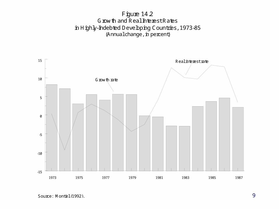
Figure 14.2Growth and Real Interest Rates

in Highly-Indebted Developing Countries, 1973-85(Annual change, in percent)

Source: Montiel (1992).

Growth rate

Real interest rate

10

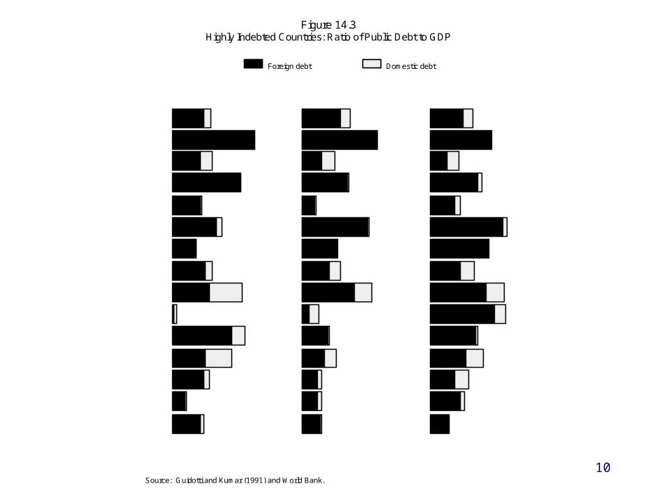
Figure 14.3Highly Indebted Countries: Ratio of Public Debt to GDP

Source: Guidotti and Kumar (1991) and World Bank.

Argentina

Bolivia

Brazil

Chile

Colombia

Côte d'Ivoire

Ecuador

Mexico

Morocco

Nigeria

Peru

Philippines

Uruguay

Venezuela

Yugoslavia

0 40 80 120

1982

Argentina

Bolivia

Brazil

Chile

Colombia

Côte d'Ivoire

Ecuador

Mexico

Morocco

Nigeria

Peru

Philippines

Uruguay

Venezuela

Yugoslavia

0 20 40 60

1976

Argentina

Bolivia

Brazil

Chile

Colombia

Côte d'Ivoire

Ecuador

Mexico

Morocco

Nigeria

Peru

Philippines

Uruguay

Venezuela

Yugoslavia

0 50 100 150

1988

Foreign debt Domestic debt

Policy Response and Macroeconomic

Implications

Resolution of the Crisis: The Brady Plan

13

Outline of the plan. Macroeconomic Effects: Conceptual Issues. An Overview of Some Early Brady Plan Deals.

14

Outline of the Plan

15

Macroeconomic Effects: Conceptual Issues

16

An Overview of Some Early Brady Plan Deals

AppendixIncentive Effects of a Debt

Overhang

18

Existence of a debt overhang creates disincentives for domestic investment in the debtor country.

Debt forgiveness can stimulate domestic investment; increase the actual payments received by creditors.

Sachs (1989b): two-period model. Debtor government maximizes the discounted utility

U() derived from domestic consumption in each period:

U(c1, c2) = u(c1) + u(c2),

u(): standard concave utility function;

ct: domestic consumption in period t,

0 < < 1: discount factor.

19

Country enters the first period with an existing stock of debt, which gives rise to a contractual payment obligation of D0 during the second period.

No debt service payments are due in the first period. Actual payments to the original creditors in the second

period are given by R, where R < D0. Actual amount to be paid emerges from negotiations

that take place between the government and its original creditors.

In the second period the government pays R to its original creditors, plus it services any additional debt it incurs from new creditors in the first period.

However, the government cannot agree to pay more than a fraction 0 < < 1 of the country's second-period income in total debt service.

20

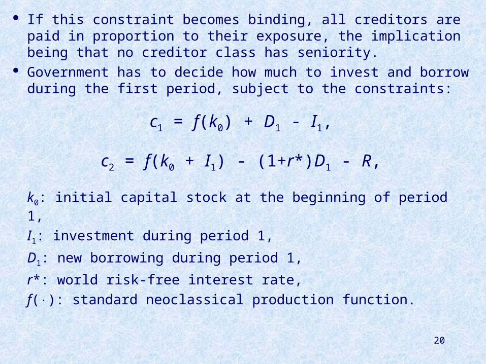
If this constraint becomes binding, all creditors are paid in proportion to their exposure, the implication being that no creditor class has seniority.

Government has to decide how much to invest and borrow during the first period, subject to the constraints:

c1 = f(k0) + D1 - I1,

c2 = f(k0 + I1) - (1+r*)D1 - R,

k0: initial capital stock at the beginning of period 1,

I1: investment during period 1,

D1: new borrowing during period 1,

r*: world risk-free interest rate,

f(): standard neoclassical production function.

21

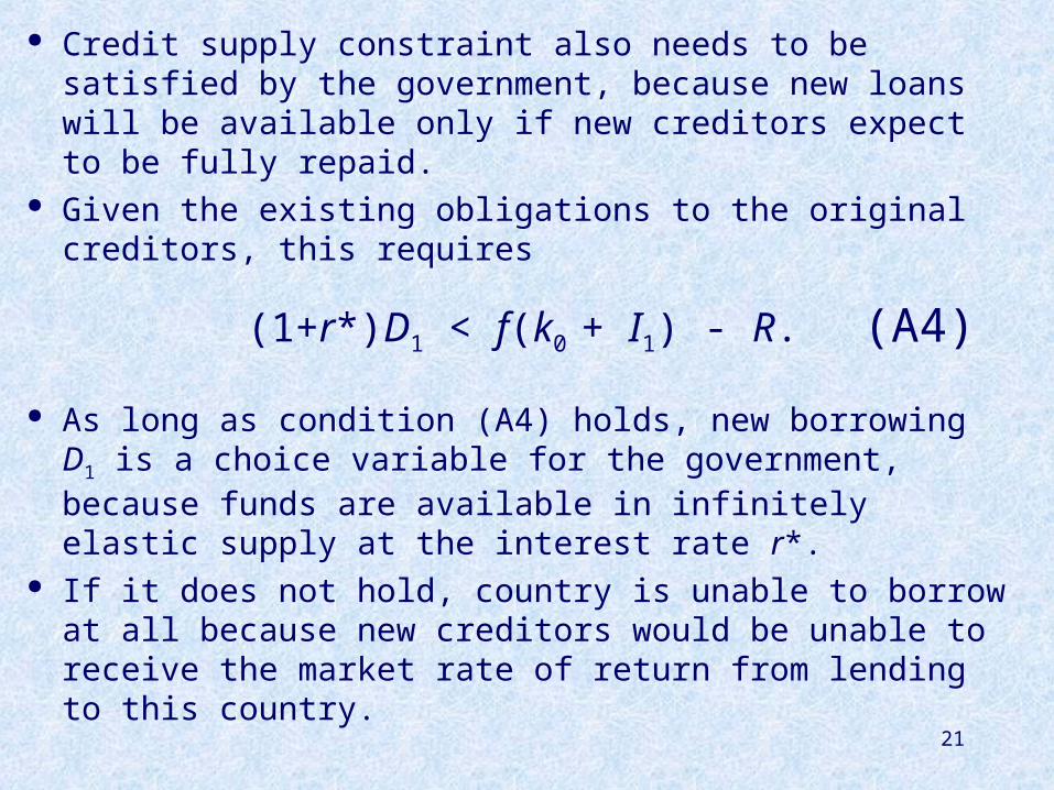
Credit supply constraint also needs to be satisfied by the government, because new loans will be available only if new creditors expect to be fully repaid.

Given the existing obligations to the original creditors, this requires

(1+r*)D1 < f(k0 + I1) - R.

As long as condition (A4) holds, new borrowing D1 is a choice variable for the government, because funds are available in infinitely elastic supply at the interest rate r*.

If it does not hold, country is unable to borrow at all because new creditors would be unable to receive the market rate of return from lending to this country.

(A4)

22

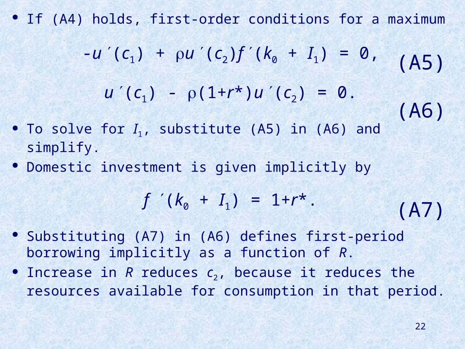
If (A4) holds, first-order conditions for a maximum

-u (c1) + u (c2)f (k0 + I1) = 0,

u (c1) - (1+r*)u (c2) = 0.

To solve for I1, substitute (A5) in (A6) and simplify. Domestic investment is given implicitly by

f (k0 + I1) = 1+r*.

Substituting (A7) in (A6) defines first-period borrowing implicitly as a function of R.

Increase in R reduces c2, because it reduces the resources available for consumption in that period.

(A5)

(A6)

(A7)

23

This raises the marginal utility of c2 and thus increases the incentive to postpone consumption.

This can be done by reducing D1. Formally,

D1 = d(R),

< 0.-f u(c2)

u(c1) + (1+r*)f u(c2) -1 < d =

24

Note that -1 < (1+r*)D1 < 0. Thus, while (A4) may hold for low values of R, an

increase in R reduces the right-hand side of (A4) more than the left-hand side.

There will thus be some critical value of R, say R*, at which (A4) will hold as an equality.

For R > R*, (A4) will be violated. Suppose that R = D0 > R*. Since all creditors would experience a shortfall, new

creditors will not enter.

25

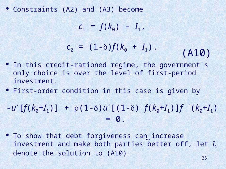
Constraints (A2) and (A3) become

c1 = f(k0) - I1,

c2 = (1-)f(k0 + I1).

In this credit-rationed regime, the government's only choice is over the level of first-period investment.

First-order condition in this case is given by

-u[f(k0+I1)] + (1-)u[(1-) f(k0+I1)]f (k0+I1) = 0.

To show that debt forgiveness can increase investment and make both parties better off, let I1 denote the solution to (A10).

(A10)

~

26

Total debt service to the original creditors in this case is R = f(k0+I1), which is less than D0 by assumption.

If the original creditors had written down the country's debt obligation to this amount initially, (A10) would become

c2 = f(k0+I1) - R,

with the first-order condition:

-u[f(k0+I1)] + (1-)u[f(k0+I1) - R]f (k0+I1) = 0.

~ ~

~

~

(A12)

(A13)

27

By substituting R= f(k0+I1) in (A13) and calculating dI1/d < 0, it is easy to show that investment increases when the contractual debt obligation is reduced from D0 to R.

Reason: When contractual debt is not fully serviced, external

creditors claim a share of any additional output forthcoming from new investment.

This is like imposing a distortionary tax in the form of the fraction in (A10), which reduces the incentive for the government to invest.

Additional investment increases domestic welfare since, by (A11), -u(c1) + u(c2)f () > 0 when this expression is evaluated at I and R, implying that additional investment is welfare enhancing.

~ ~

~

~ ~

28

Result: debt forgiveness increases domestic welfare without harming the original creditors; that is, debt forgiveness is Pareto-improving.

With an increase in R to above R (but below D0), debtor country could remain better off than in the no-forgiveness condition.

Value of debt service to original creditors increases over what they would have received without debt forgiveness.

Result: removing distortionary effect of the debt overhang can make both parties better off.

~