1 bayesian classification instructor: qiang yang hong kong university of science and technology...
Post on 19-Dec-2015
217 views
TRANSCRIPT

1
Bayesian Classification
Instructor: Qiang YangHong Kong University of Science and Technology
Thanks: Dan Weld, Eibe Frank
3
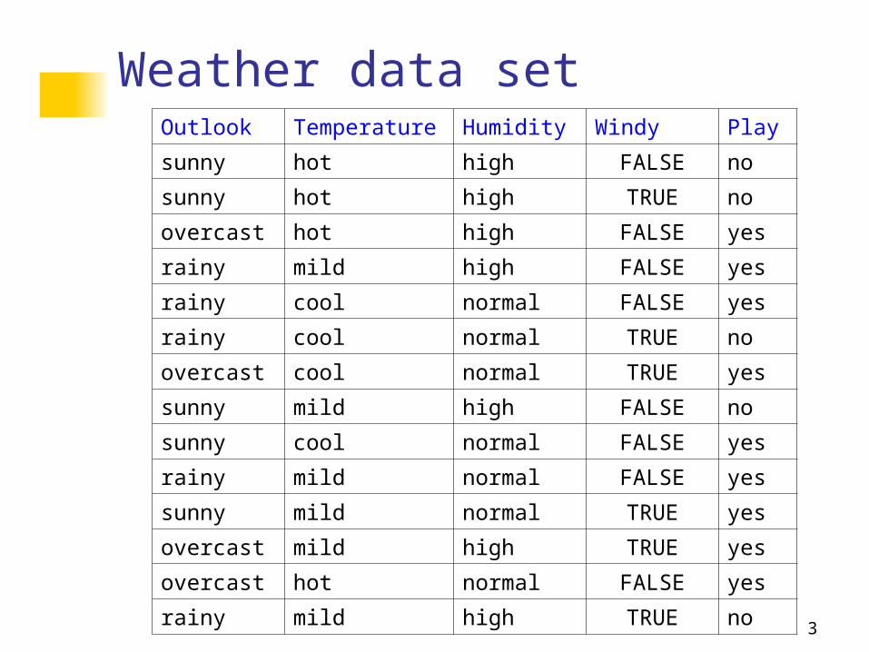
Weather data setOutlook Temperature Humidity Windy Play
sunny hot high FALSE no
sunny hot high TRUE no
overcast hot high FALSE yes
rainy mild high FALSE yes
rainy cool normal FALSE yes
rainy cool normal TRUE no
overcast cool normal TRUE yes
sunny mild high FALSE no
sunny cool normal FALSE yes
rainy mild normal FALSE yes
sunny mild normal TRUE yes
overcast mild high TRUE yes
overcast hot normal FALSE yes
rainy mild high TRUE no
4
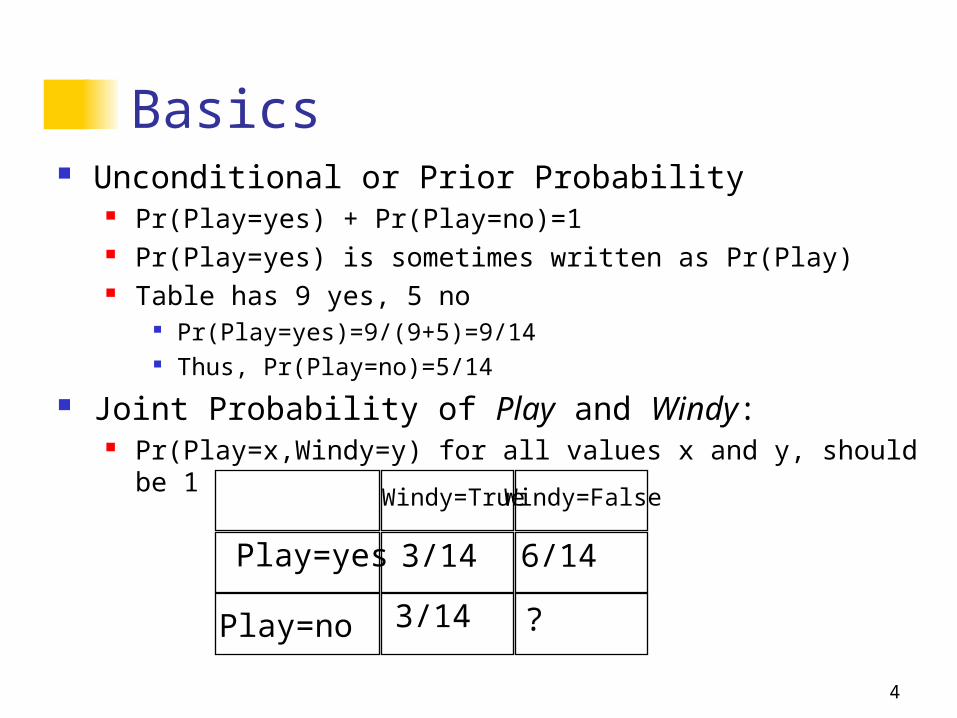
Basics Unconditional or Prior Probability
Pr(Play=yes) + Pr(Play=no)=1 Pr(Play=yes) is sometimes written as Pr(Play) Table has 9 yes, 5 no
Pr(Play=yes)=9/(9+5)=9/14 Thus, Pr(Play=no)=5/14
Joint Probability of Play and Windy: Pr(Play=x,Windy=y) for all values x and y, should be 1
Play=yes
Play=no
Windy=True Windy=False
3/14
?3/14
6/14
5
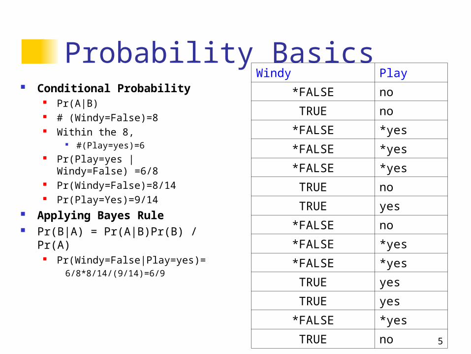
Probability Basics Conditional Probability
Pr(A|B) # (Windy=False)=8 Within the 8,
#(Play=yes)=6 Pr(Play=yes | Windy=False)
=6/8 Pr(Windy=False)=8/14 Pr(Play=Yes)=9/14
Applying Bayes Rule Pr(B|A) = Pr(A|B)Pr(B) /
Pr(A) Pr(Windy=False|Play=yes)=
6/8*8/14/(9/14)=6/9
Windy Play
*FALSE no
TRUE no
*FALSE *yes
*FALSE *yes
*FALSE *yes
TRUE no
TRUE yes
*FALSE no
*FALSE *yes
*FALSE *yes
TRUE yes
TRUE yes
*FALSE *yes
TRUE no
6
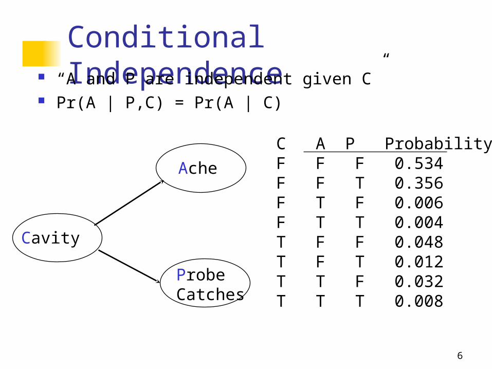
Conditional Independence “ A and P are independent given C” Pr(A | P,C) = Pr(A | C)
Cavity
ProbeCatches
Ache
C A P ProbabilityF F F 0.534F F T 0.356F T F 0.006F T T 0.004T F F 0.048T F T 0.012T T F 0.032T T T 0.008

7
Pr(A|C) = 0.032+0.008/ (0.048+0.012+0.032+0.008)
= 0.04 / 0.1 = 0.4
Suppose C=TruePr(A|P,C) = 0.032/(0.032+0.048)
= 0.032/0.080 = 0.4
Conditional Independence “ A and P are independent given C” Pr(A | P,C) = Pr(A | C) and also Pr(P | A,C) = Pr(P | C)
C A P ProbabilityF F F 0.534F F T 0.356F T F 0.006F T T 0.004T F F 0.012T F T 0.048T T F 0.008T T T 0.032
8
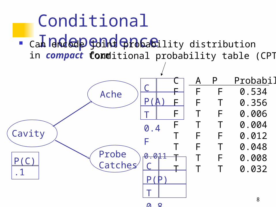
Conditional Independence Can encode joint probability distribution in compact form
C A P ProbabilityF F F 0.534F F T 0.356F T F 0.006F T T 0.004T F F 0.012T F T 0.048T T F 0.008T T T 0.032
Cavity
ProbeCatches
Ache
P(C).1
C P(P)
T 0.8
F 0.4
C P(A)
T 0.4
F 0.011
Conditional probability table (CPT)
9
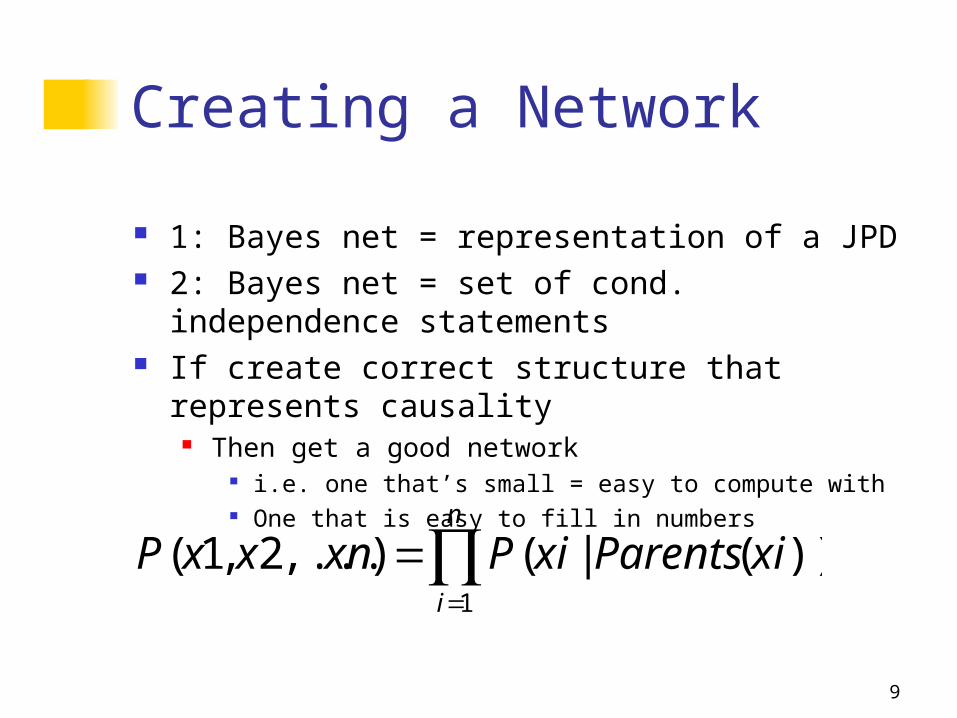
Creating a Network
1: Bayes net = representation of a JPD 2: Bayes net = set of cond. independence
statements If create correct structure that represents
causality Then get a good network
i.e. one that’s small = easy to compute with One that is easy to fill in numbers
n
i
xiParentsxiPxnxxP1
))(|(),...2,1(
10
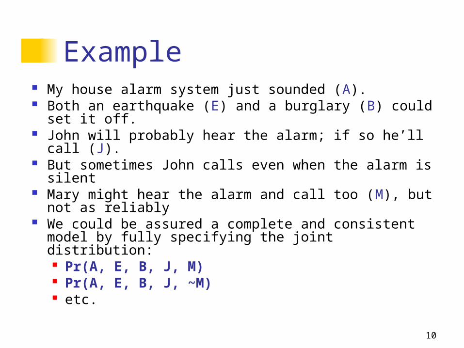
Example My house alarm system just sounded (A). Both an earthquake (E) and a burglary (B) could
set it off. John will probably hear the alarm; if so he’ll call (J). But sometimes John calls even when the alarm is
silent Mary might hear the alarm and call too (M), but
not as reliably We could be assured a complete and consistent
model by fully specifying the joint distribution: Pr(A, E, B, J, M) Pr(A, E, B, J, ~M) etc.
11
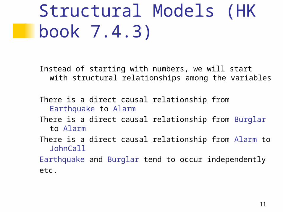
Structural Models (HK book 7.4.3)
Instead of starting with numbers, we will start with structural relationships among the variables
There is a direct causal relationship from Earthquake to Alarm
There is a direct causal relationship from Burglar to Alarm
There is a direct causal relationship from Alarm to JohnCallEarthquake and Burglar tend to occur independentlyetc.
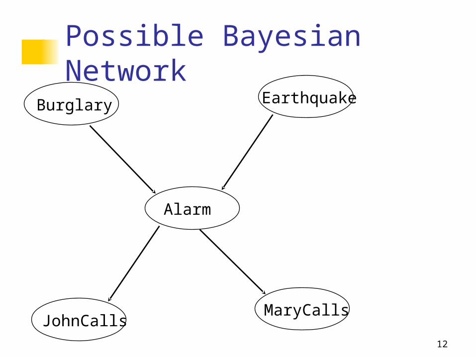
12
Possible Bayesian Network
Burglary
MaryCallsJohnCalls
Alarm
Earthquake
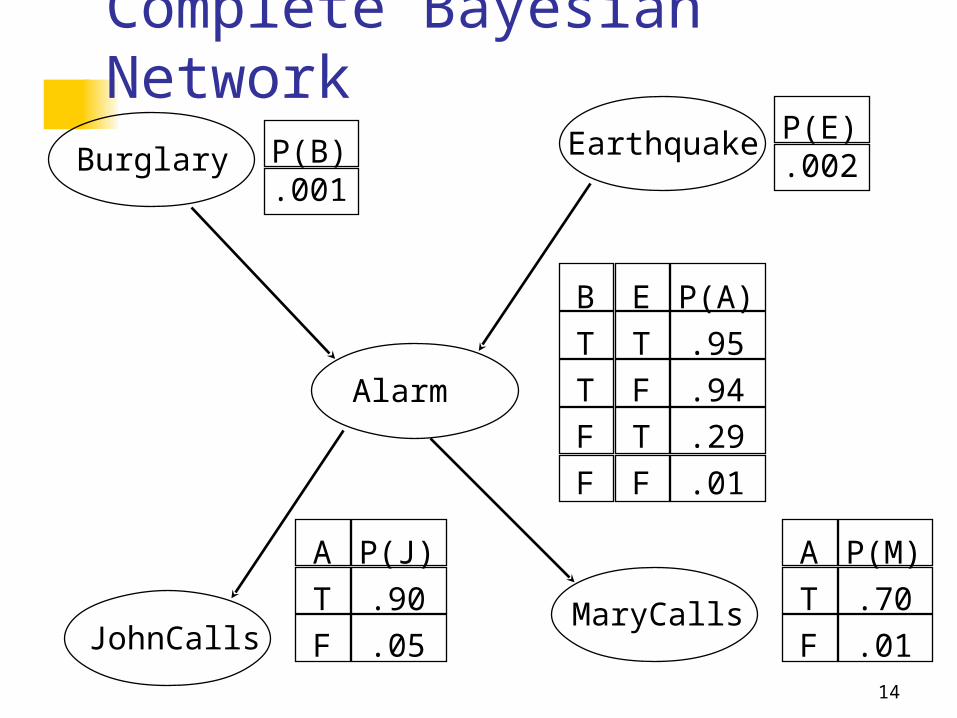
14
Complete Bayesian Network
Burglary
MaryCallsJohnCalls
Alarm
Earthquake
P(A)
.95
.94
.29
.01
A
T
F
P(J)
.90
.05
A
T
F
P(M)
.70
.01
P(B).001
P(E).002
E
T
F
T
F
B
T
T
F
F
15
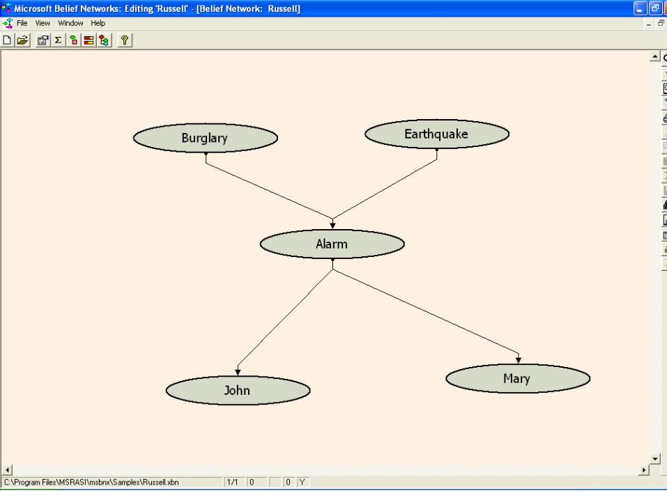
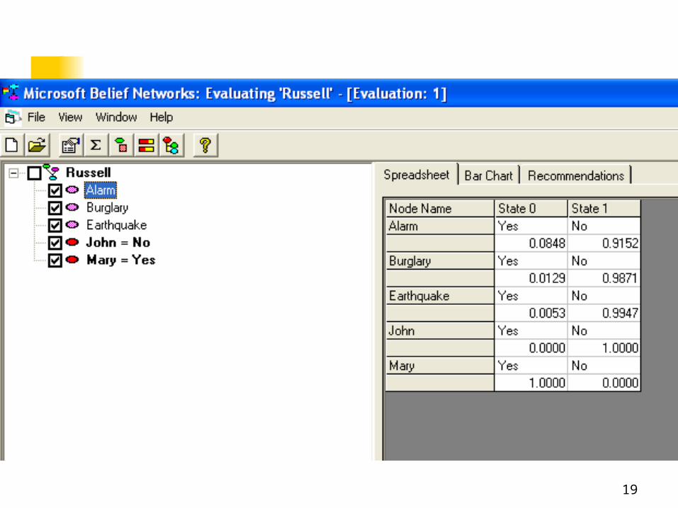
Microsoft Bayesian Belief Net
http://research.microsoft.com/adapt/MSBNx/ Can be used to construct and reason with
Bayesian Networks Consider the example
16

17

18
19
20
Mining for Structural Models
Difficult to mine Some methods are proposed Up to now, no good results yet
Often requires domain expert’s knowledge Once set up, a Bayesian Network can be used
to provide probabilistic queries Microsoft Bayesian Network Software
21
Use the Bayesian Net for Prediction From a new day’s data we wish to predict the
decision New data: X Class label: C To predict the class of X, is the same as asking
Value of Pr(C|X)? Pr(C=yes|X) Pr(C=no|X) Compare the two
22
Naïve Bayesian Models Two assumptions: Attributes are
equally important statistically independent (given the class
value) This means that knowledge about the value of a
particular attribute doesn’t tell us anything about the value of another attribute (if the class is known)
Although based on assumptions that are almost never correct, this scheme works well in practice!
23
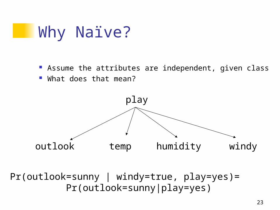
Why Naïve?
Assume the attributes are independent, given class What does that mean?
play
outlook temp humidity windy
Pr(outlook=sunny | windy=true, play=yes)= Pr(outlook=sunny|play=yes)
24
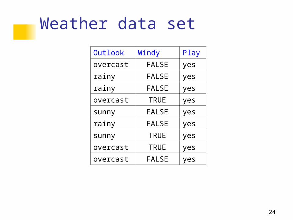
Weather data set
Outlook Windy Play
overcast FALSE yes
rainy FALSE yes
rainy FALSE yes
overcast TRUE yes
sunny FALSE yes
rainy FALSE yes
sunny TRUE yes
overcast TRUE yes
overcast FALSE yes
25
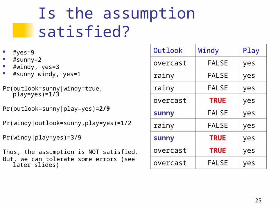
Is the assumption satisfied? #yes=9 #sunny=2 #windy, yes=3 #sunny|windy, yes=1
Pr(outlook=sunny|windy=true, play=yes)=1/3
Pr(outlook=sunny|play=yes)=2/9
Pr(windy|outlook=sunny,play=yes)=1/2
Pr(windy|play=yes)=3/9
Thus, the assumption is NOT satisfied.But, we can tolerate some errors (see later
slides)
Outlook Windy Play
overcast FALSE yes
rainy FALSE yes
rainy FALSE yes
overcast TRUE yes
sunny FALSE yes
rainy FALSE yes
sunny TRUE yes
overcast TRUE yes
overcast FALSE yes
26
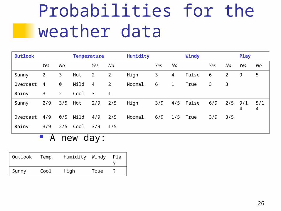
Probabilities for the weather data
Outlook Temperature Humidity Windy Play
Yes No Yes No Yes No Yes No Yes No
Sunny 2 3 Hot 2 2 High 3 4 False 6 2 9 5
Overcast 4 0 Mild 4 2 Normal 6 1 True 3 3
Rainy 3 2 Cool 3 1
Sunny 2/9 3/5 Hot 2/9 2/5 High 3/9 4/5 False 6/9 2/5 9/14 5/14
Overcast 4/9 0/5 Mild 4/9 2/5 Normal 6/9 1/5 True 3/9 3/5
Rainy 3/9 2/5 Cool 3/9 1/5
Outlook Temp. Humidity Windy Play
Sunny Cool High True ?
A new day:
27
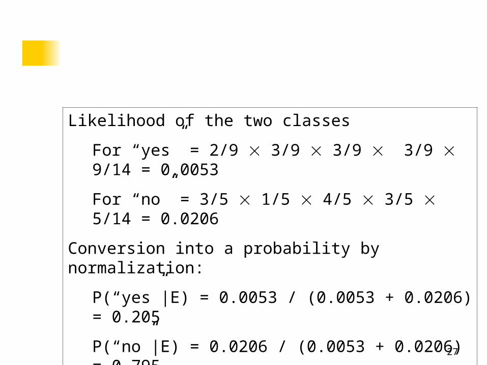
Likelihood of the two classes
For “yes” = 2/9 3/9 3/9 3/9 9/14 = 0.0053
For “no” = 3/5 1/5 4/5 3/5 5/14 = 0.0206
Conversion into a probability by normalization:
P(“yes”|E) = 0.0053 / (0.0053 + 0.0206) = 0.205
P(“no”|E) = 0.0206 / (0.0053 + 0.0206) = 0.795
28
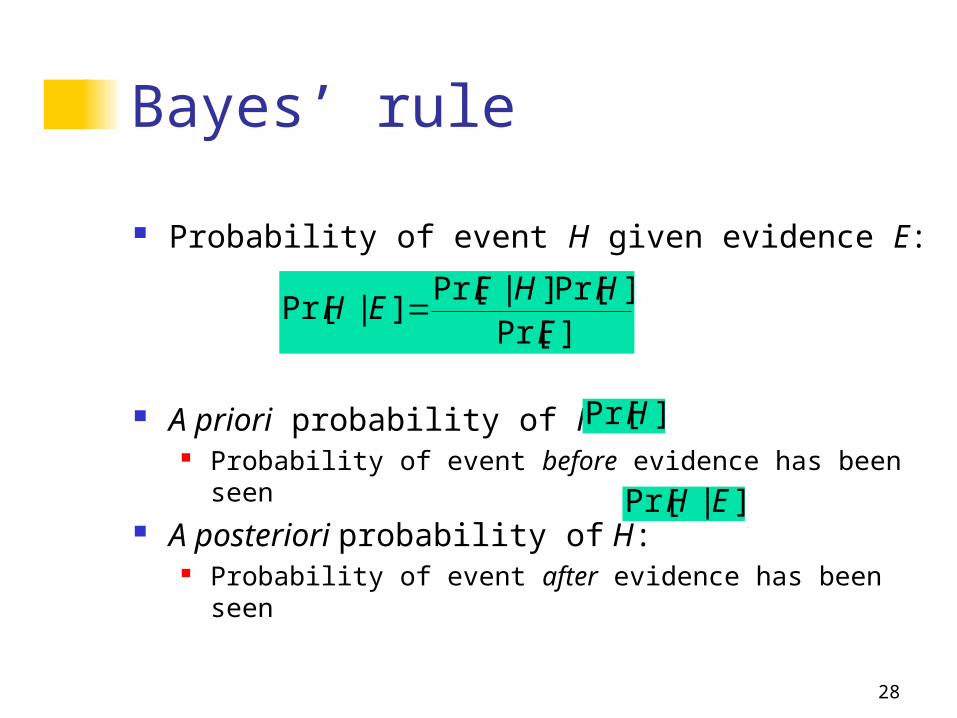
Bayes’ rule
Probability of event H given evidence E:
A priori probability of H: Probability of event before evidence has been seen
A posteriori probability of H: Probability of event after evidence has been seen
]Pr[]Pr[]|Pr[
]|Pr[E
HHEEH
]|Pr[ EH
]Pr[H
29
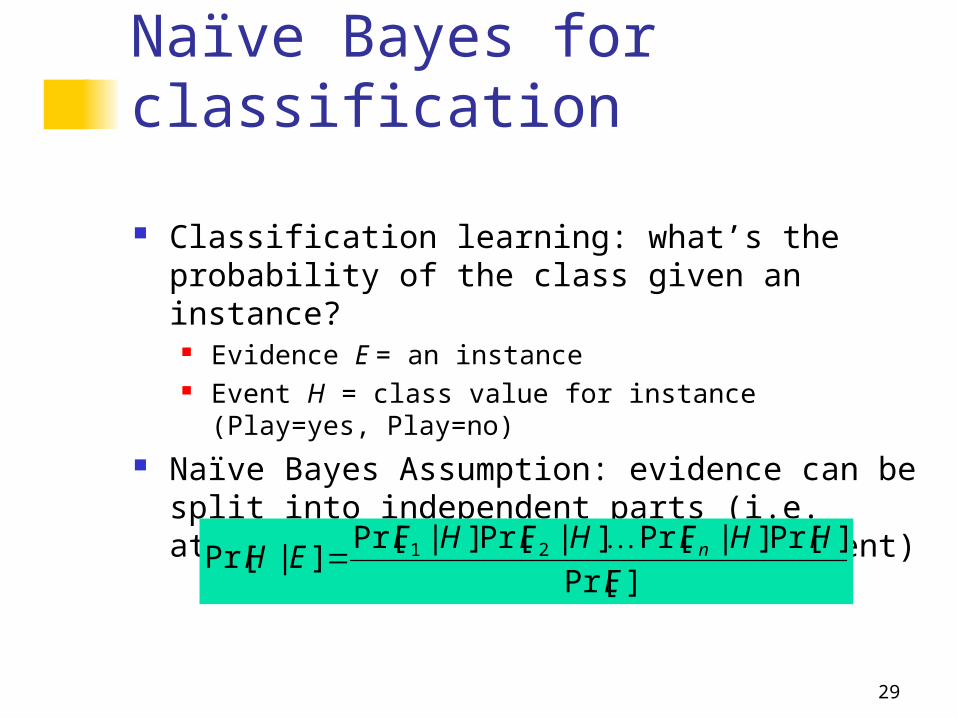
Naïve Bayes for classification
Classification learning: what’s the probability of the class given an instance?
Evidence E = an instance Event H = class value for instance (Play=yes,
Play=no) Naïve Bayes Assumption: evidence can be split
into independent parts (i.e. attributes of instance are independent)
]Pr[
]Pr[]|Pr[]|Pr[]|Pr[]|Pr[ 21
E
HHEHEHEEH n
30
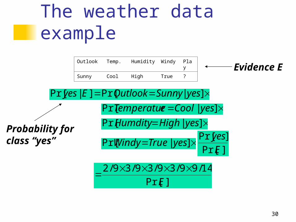
The weather data exampleOutlook Temp. Humidity Windy Play
Sunny Cool High True ?
]|Pr[]|Pr[ yesSunnyOutlookEyes
]|Pr[ yesCooleTemperatur
]|Pr[ yesHighHumdity
]|Pr[ yesTrueWindy]Pr[]Pr[
Eyes
]Pr[14/99/39/39/39/2
E
Evidence E
Probability forclass “yes”
31
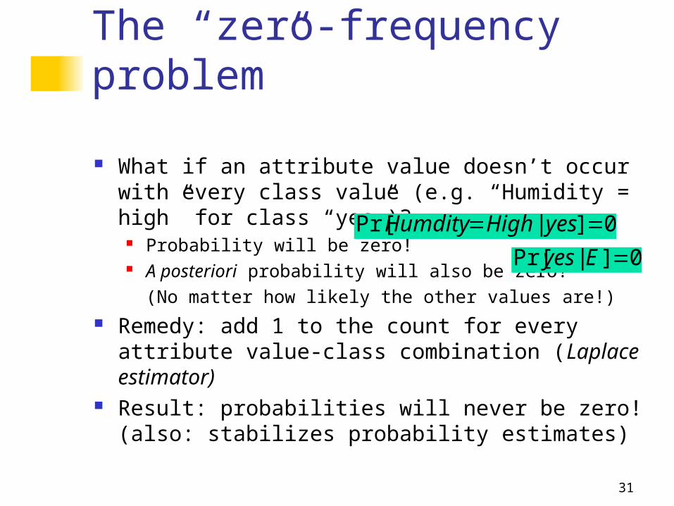
The “zero-frequency problem”
What if an attribute value doesn’t occur with every class value (e.g. “Humidity = high” for class “yes”)?
Probability will be zero! A posteriori probability will also be zero!
(No matter how likely the other values are!) Remedy: add 1 to the count for every attribute
value-class combination (Laplace estimator) Result: probabilities will never be zero! (also:
stabilizes probability estimates)
0]|Pr[ yesHighHumdity
0]|Pr[ Eyes
32
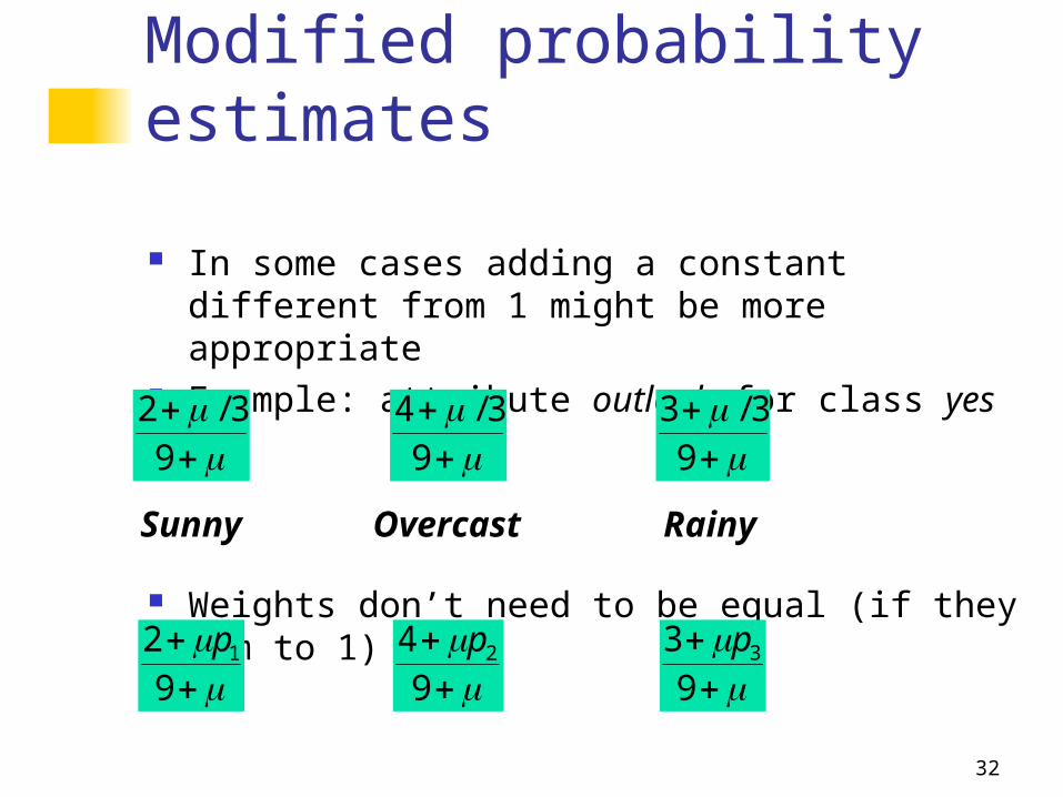
Modified probability estimates
In some cases adding a constant different from 1 might be more appropriate
Example: attribute outlook for class yes
Weights don’t need to be equal (if they sum to 1)
9
3/2
9
3/4
9
3/3
Sunny Overcast Rainy
92 1p
9
4 2p
9
3 3p
33
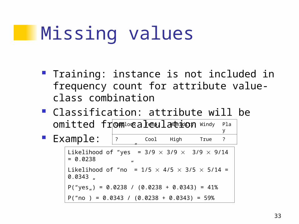
Missing values
Training: instance is not included in frequency count for attribute value-class combination
Classification: attribute will be omitted from calculation
Example: Outlook Temp. Humidity Windy Play
? Cool High True ?
Likelihood of “yes” = 3/9 3/9 3/9 9/14 = 0.0238
Likelihood of “no” = 1/5 4/5 3/5 5/14 = 0.0343
P(“yes”) = 0.0238 / (0.0238 + 0.0343) = 41%
P(“no”) = 0.0343 / (0.0238 + 0.0343) = 59%
34
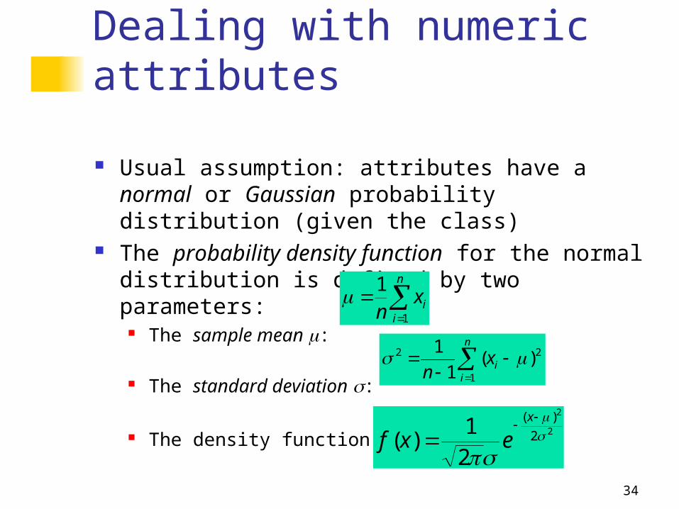
Dealing with numeric attributes
Usual assumption: attributes have a normal or Gaussian probability distribution (given the class)
The probability density function for the normal distribution is defined by two parameters:
The sample mean :
The standard deviation :
The density function f(x):
n
iixn 1
1
n
iixn 1
22 )(1
1
2
2
2
)(
21
)(
x
exf
35
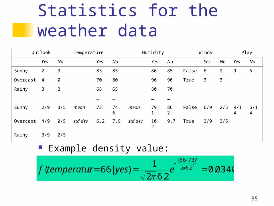
Statistics for the weather data
Example density value:
Outlook Temperature Humidity Windy Play
Yes No Yes No Yes No Yes No Yes No
Sunny 2 3 83 85 86 85 False 6 2 9 5
Overcast 4 0 70 80 96 90 True 3 3
Rainy 3 2 68 65 80 70
… … … …
Sunny 2/9 3/5 mean 73 74.6 mean 79.1 86.2 False 6/9 2/5 9/14 5/14
Overcast 4/9 0/5 std dev 6.2 7.9 std dev 10.2 9.7 True 3/9 3/5
Rainy 3/9 2/5
0340.02.62
1)|66(
2
2
2.62
)7366(
eyesetemperaturf
36
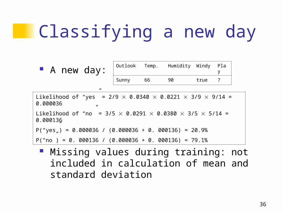
Classifying a new day
A new day:
Missing values during training: not included in calculation of mean and standard deviation
Outlook Temp. Humidity Windy Play
Sunny 66 90 true ?
Likelihood of “yes” = 2/9 0.0340 0.0221 3/9 9/14 = 0.000036
Likelihood of “no” = 3/5 0.0291 0.0380 3/5 5/14 = 0.000136
P(“yes”) = 0.000036 / (0.000036 + 0. 000136) = 20.9%
P(“no”) = 0. 000136 / (0.000036 + 0. 000136) = 79.1%
37
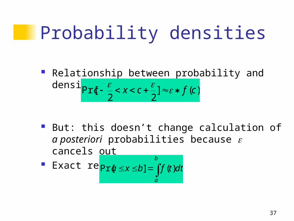
Probability densities
Relationship between probability and density:
But: this doesn’t change calculation of a posteriori probabilities because cancels out
Exact relationship:
)(]22
Pr[ cfcxc
b
a
dttfbxa )(]Pr[
38
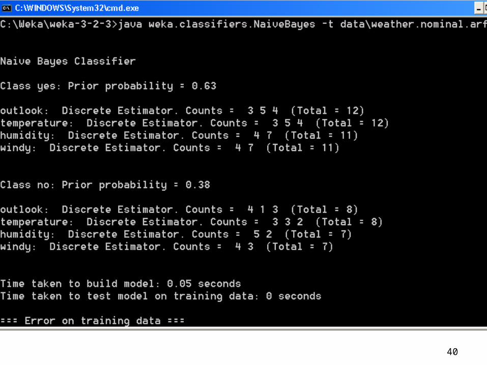
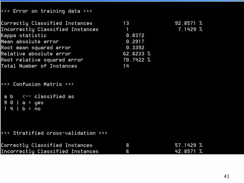
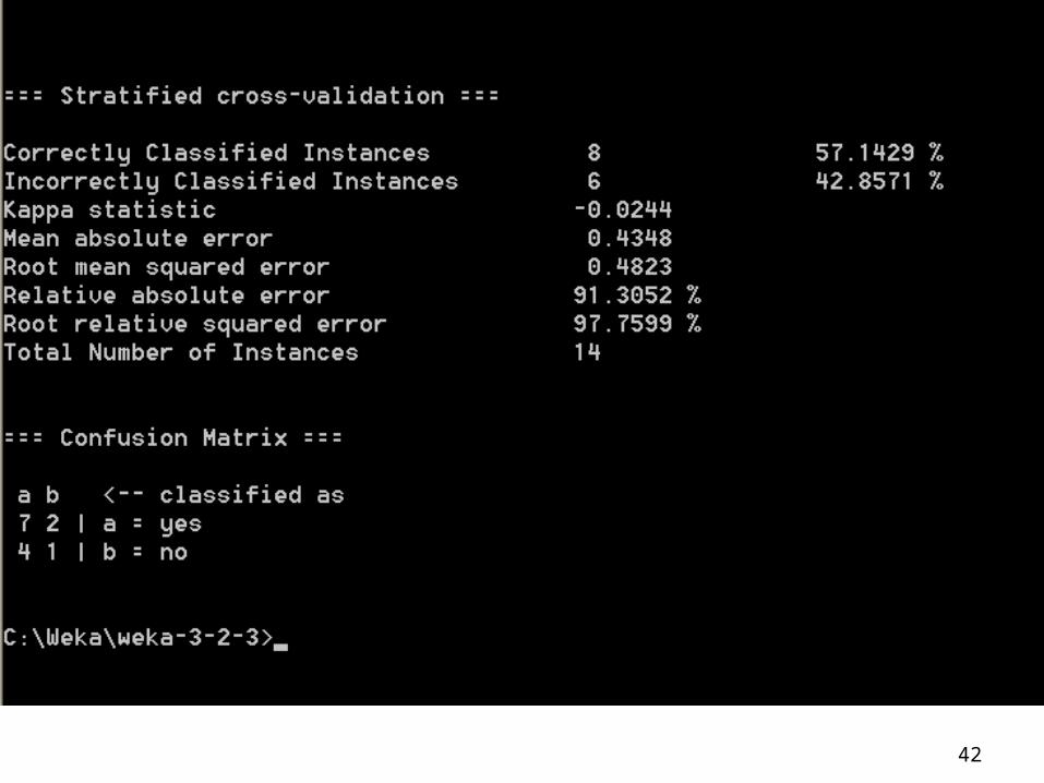
Example of Naïve Bayes in Weka
Use Weka Naïve Bayes Module to classify Weather.nominal.arff

39
40
41
42
43
Discussion of Naïve Bayes
Naïve Bayes works surprisingly well (even if independence assumption is clearly violated)
Why? Because classification doesn’t require accurate probability estimates as long as maximum probability is assigned to correct class
However: adding too many redundant attributes will cause problems (e.g. identical attributes)
Note also: many numeric attributes are not normally distributed