–1–

3dDeconvolve3dDeconvolveAdvanced Features

Et cetera

Just in case you werenJust in case you weren’’ttconfused enough alreadyconfused enough already

–2–

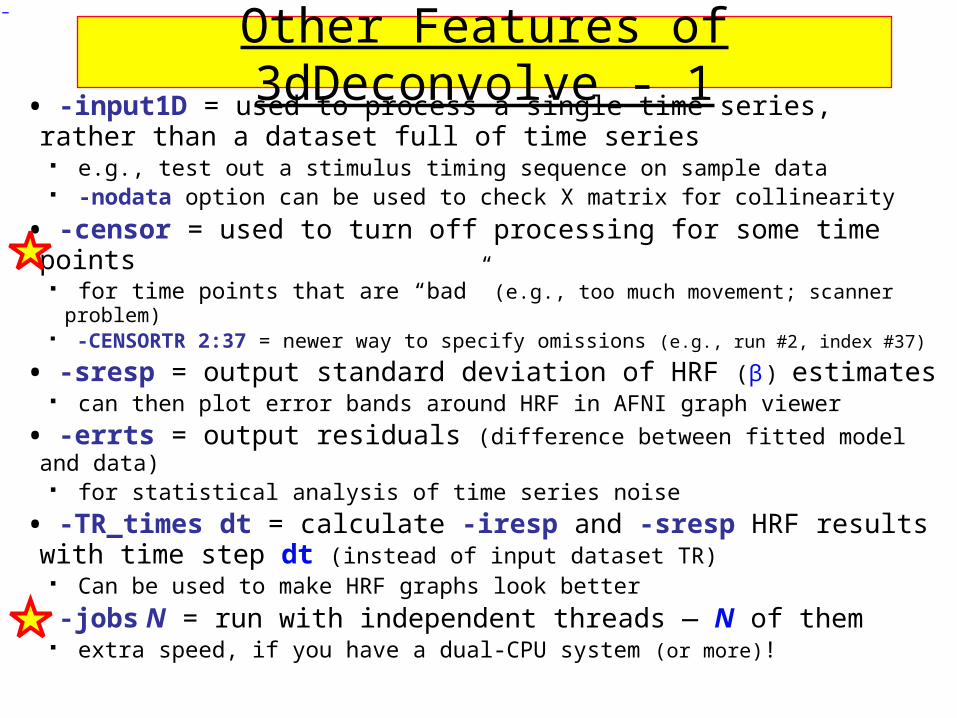
Other Features of 3dDeconvolve - 1• -input1D = used to process a single time series, rather than a dataset full of time series e.g., test out a stimulus timing sequence on sample data -nodata option can be used to check X matrix for collinearity

• -censor = used to turn off processing for some time points for time points that are “bad” (e.g., too much movement; scanner problem) -CENSORTR 2:37 = newer way to specify omissions (e.g., run #2, index #37)

• -sresp = output standard deviation of HRF (β ) estimates can then plot error bands around HRF in AFNI graph viewer

• -errts = output residuals (difference between fitted model and data) for statistical analysis of time series noise

• -TR_times dt = calculate -iresp and -sresp HRF results with time step dt (instead of input dataset TR) Can be used to make HRF graphs look better

• -jobs N = run with independent threads — N of them extra speed, if you have a dual-CPU system (or more)!

–3–

http://afni.nimh.nih.gov/pub/dist/doc/misc/Decon/DeconSummer2004.html http://afni.nimh.nih.gov/pub/dist/doc/misc/Decon/DeconSpring2007.html

• Equation solver: Program computes condition number for X matrix (measures of how sensitive regression results are to changes in X) If the condition number is “bad” (too big), then the program will not actually proceed to compute the results

You can use the -GOFORIT option on the command line to force the program to run despite X matrix warnings

o But you should strive to understand why you are getting these warnings!!

• Other matrix checks: Duplicate stimulus filenames, duplicate regression matrix columns, all zero matrix columns

• Check the screen output for WARNINGs and ERRORs Such messages also saved into file 3dDeconvolve.err

Other Features - 2

–4–

Other Features - 3• All-zero regressors are allowed (via -allzero_OK or -GOFORIT)

Will get zero weight in the solution Example: task where subject makes a choice for each stimulus (e.g., male or female face?)

o You want to analyze correct and incorrect trials as separate caseso What if some subject makes no mistakes? Hmmm…

Can keep the all-zero regressor (e.g., all -stim_times = *) Input files and output datasets for error-making and perfect-

performing subjects will be organized the same way

• 3dDeconvolve_f program can be used to compute linear regression results in single precision (7 decimal places) rather than double precision (16 places) For better speed, but with lower numerical accuracy Best to do at least one run both ways to check if results differ significantly (Equation solver should be safe, but …)

–6–

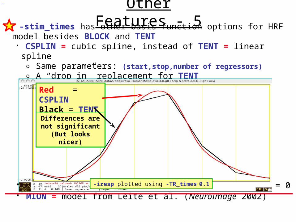
• -stim_times has other basis function options for HRF model besides BLOCK and TENT CSPLIN = cubic spline, instead of TENT = linear spline

o Same parameters: (start,stop,number of regressors) o A “drop in” replacement for TENT

TENTzero & CSPLINzero = force start & end of HRF = 0 MION = model from Leite et al. (NeuroImage 2002)

Other Features - 5

Red = CSPLINBlack = TENTDifferences are not

significant(But looks nicer)

-iresp plotted using -TR_times 0.1

–7–

Other Features - 6• -fitts option is used to create a synthetic dataset

each voxel time series is full (signal+baseline) model as fitted to the data time series in the corresponding voxel location

• 3dSynthesize program can be used to create synthetic datasets from subsets of the full model Uses -x1D and -cbucket outputs from 3dDeconvolve

o -cbucket stores β coefficients for each X matrix column into dataseto -x1D stores the matrix columns (and -stim_labels, etc.)

Potential uses:o Baseline only dataset

3dSynthesize -cbucket fred+orig -matrix fred.xmat.1D -select baseline -prefix fred_base

Could subtract this dataset from original data (via 3dcalc) to get signal+noise dataset that has no baseline component left

o Just one stimulus class model (+ baseline) dataset 3dSynthesize -cbucket fred+orig -matrix fred.xmat.1D -select baseline Faces -prefix fred_Faces

–9–

• IM = Individual Modulation Compute separate amplitude of response for each

stimuluso Instead of computing average amplitude of

responses to multiple stimuli in the same class Response amplitudes (βs) for each individual

block/event will be highly noisyo Can’t use individual activation map for mucho Must pool the computed βs in some further

statistical analysis (t-test via 3dttest? inter-voxel correlations in the βs? Correlate βs with something else?)

Usage: -stim_times_IM k tname modelo Like -stim_times, but creates a separate

regression matrix column for each time given

IMIM Regression - 1 Regression - 1

–10–

• First application of IM was checking some data we received from another institution• Experiment: 64 blocks of sensorimotor task (8 runs

each with 8 blocks)

IMIM Regression - 2 Regression - 2

Plot of 64 BLOCK s from -cbucket output

N.B.: sign reversal in run #4 = stimulus timing error!

–11–

• IM works naturally with blocks, which only have 1 amplitude parameter per stimulus• With event-related experiment and deconvolution,

have multiple amplitude parameters per stimulus Difficulty: each event in same class won’t get the

same shaped HRF this way Desideratum: allow response shape to vary (that’s

deconvolution), but only allow amplitude to vary between responses in the same stimulus class

Problem: get unknowns that multiply each other (shape parameters × amplitude parameters) — and we step outside the realm of linear analysis

Possible solution: semi-linear regression (nonlinear in global shape parameters, linear in local amplitude params)

IMIM Regression - 3 Regression - 3

–12–

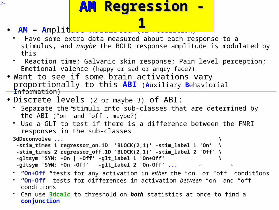
• AM = Amplitude Modulated (or Modulation) Have some extra data measured about each response to a stimulus,

and maybe the BOLD response amplitude is modulated by this Reaction time; Galvanic skin response; Pain level perception;

Emotional valence (happy or sad or angry face?)

• Want to see if some brain activations vary proportionally to this ABI (Auxiliary Behaviorial Information)• Discrete levels (2 or maybe 3) of ABI:

Separate the stimuli into sub-classes that are determined by the ABI (“on” and “off”, maybe?)

Use a GLT to test if there is a difference between the FMRI responses in the sub-classes

3dDeconvolve ... \ -stim_times 1 regressor_on.1D 'BLOCK(2,1)' -stim_label 1 'On' \ -stim_times 2 regressor_off.1D 'BLOCK(2,1)' -stim_label 2 'Off' \ -gltsym 'SYM: +On | +Off' -glt_label 1 'On+Off' \ -gltsym 'SYM: +On -Off' -glt_label 2 'On-Off' ... “On+Off” tests for any activation in either the “on” or “off” conditions “On-Off” tests for differences in activation between “on” and “off” conditions Can use 3dcalc to threshold on both statistics at once to find a conjunction

AMAM Regression - 1 Regression - 1

–13–

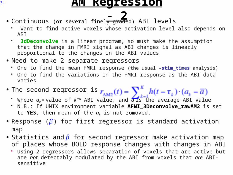
• Continuous (or several finely graded) ABI levels Want to find active voxels whose activation level also depends on ABI 3dDeconvolve is a linear program, so must make the assumption that

the change in FMRI signal as ABI changes is linearly proportional to the changes in the ABI values

• Need to make 2 separate regressors One to find the mean FMRI response (the usual -stim_times analysis) One to find the variations in the FMRI response as the ABI data varies

• The second regressor is Where ak = value of k th ABI value, and a is the average ABI value N.B.: If UNIX environment variable AFNI_3Deconvolve_rawAM2 is set

to YES, then mean of the ak is not removed.

• Response (β ) for first regressor is standard activation map• Statistics and β for second regressor make activation map of

places whose BOLD response changes with changes in ABI Using 2 regressors allows separation of voxels that are active but are

not detectably modulated by the ABI from voxels that are ABI-sensitive

AM Regression - 2

–14–

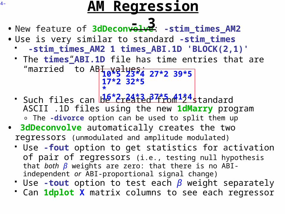
• New feature of 3dDeconvolve: -stim_times_AM2• Use is very similar to standard -stim_times

-stim_times_AM2 1 times_ABI.1D 'BLOCK(2,1)' The times_ABI.1D file has time entries that are “married”

to ABI values:

Such files can be created from 2 standard ASCII .1D files using the new 1dMarry programo The -divorce option can be used to split them up

• 3dDeconvolve automatically creates the two regressors (unmodulated and amplitude modulated) Use -fout option to get statistics for activation of pair of

regressors (i.e., testing null hypothesis that both β weights are zero: that there is no ABI-independent or ABI-proportional signal change)

Use -tout option to test each β weight separately Can 1dplot X matrix columns to see each regressor

AM Regression - 3

10*5 23*4 27*2 39*517*2 32*5*16*2 24*3 37*5 41*4

–15–

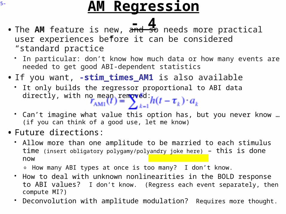
• The AM feature is new, and so needs more practical user experiences before it can be considered “standard practice” In particular: don’t know how much data or how many events are

needed to get good ABI-dependent statistics

• If you want, -stim_times_AM1 is also available It only builds the regressor proportional to ABI data directly, with no

mean removed:

Can’t imagine what value this option has, but you never know … (if you can think of a good use, let me know)

• Future directions: Allow more than one amplitude to be married to each stimulus time

(insert obligatory polygamy/polyandry joke here) – this is done nowo How many ABI types at once is too many? I don’t know.

How to deal with unknown nonlinearities in the BOLD response to ABI values? I don’t know. (Regress each event separately, then compute MI?)

Deconvolution with amplitude modulation? Requires more thought.

AM Regression - 4

–16–

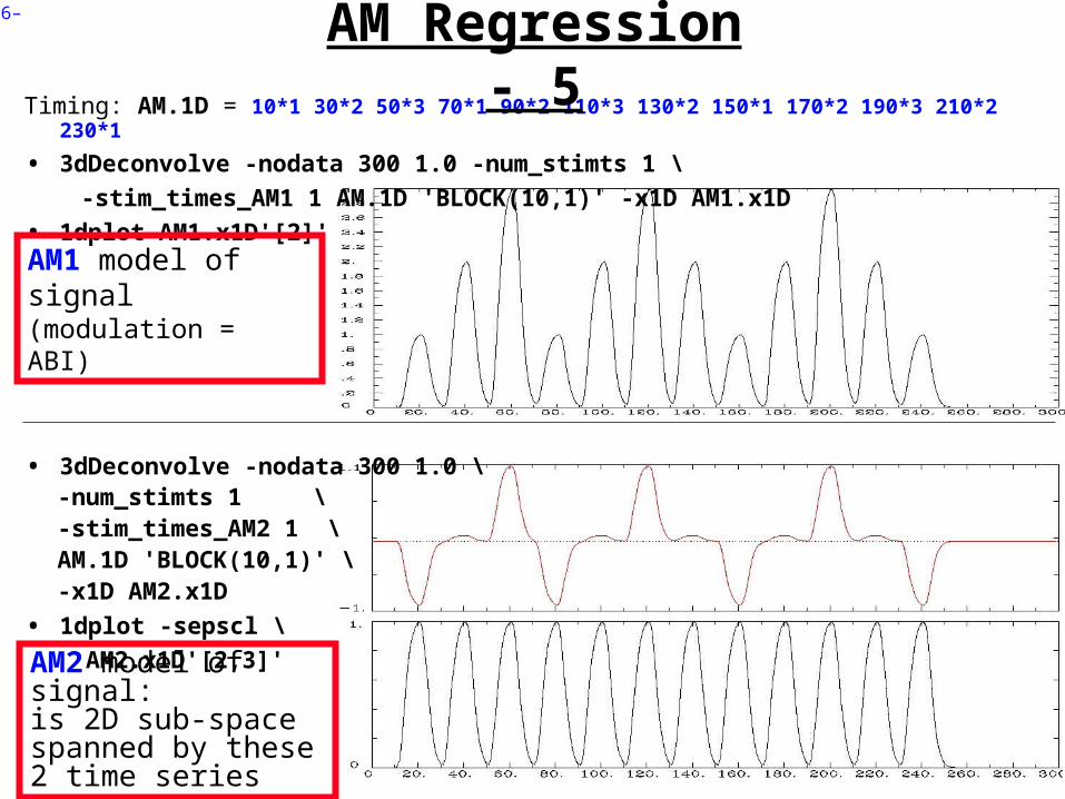
Timing: AM.1D = 10*1 30*2 50*3 70*1 90*2 110*3 130*2 150*1 170*2 190*3 210*2 230*1

• 3dDeconvolve -nodata 300 1.0 -num_stimts 1 \

-stim_times_AM1 1 AM.1D 'BLOCK(10,1)' -x1D AM1.x1D

• 1dplot AM1.x1D'[2]'

• 3dDeconvolve -nodata 300 1.0 \-num_stimts 1 \-stim_times_AM2 1 \ AM.1D 'BLOCK(10,1)' \ -x1D AM2.x1D

• 1dplot -sepscl \

AM2.x1D'[2,3]'

AM Regression - 5

AM1 model of signal (modulation = ABI)

AM2 model of signal:is 2D sub-space spanned by these 2 time series

–17–

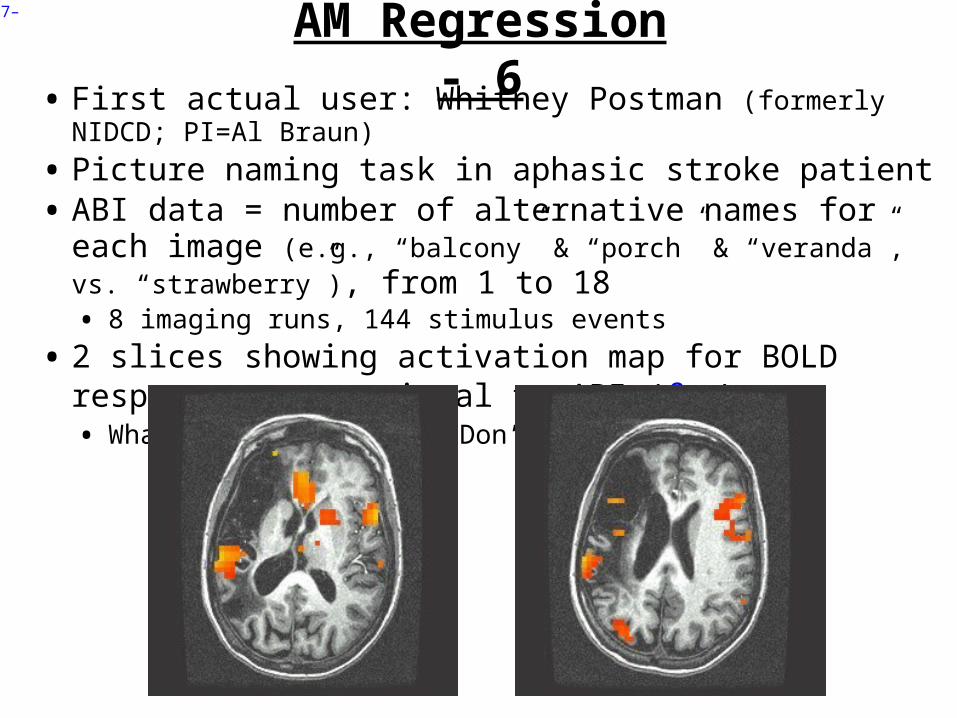
• First actual user: Whitney Postman (formerly NIDCD; PI=Al Braun)

• Picture naming task in aphasic stroke patient• ABI data = number of alternative names for each image (e.g.,

“balcony” & “porch” & “veranda”, vs. “strawberry”), from 1 to 18• 8 imaging runs, 144 stimulus events

• 2 slices showing activation map for BOLD responses proportional to ABI (βAM2)• What does this mean? Don’t ask me!

AM Regression - 6

–18–

• Alternative: use IM to get individual βs for each block/event and then do external regression statistics on those values• Could do nonlinear fitting (to these βs) via 3dNLfim,

or inter-class contrasts via 3dttest, 3dLME, 3dANOVA, or intra-class correlations via 3dICC, etc.• What is better: AM or IM+something more ?• We don’t know – experience with these options is

limited thus far – you can always try both!• If AM doesn’t fit your models/ideas, then IM+ is

clearly the way to go• Probably need to consult with SSCC to get some

hints/advice

AM Regression - 7

–19–

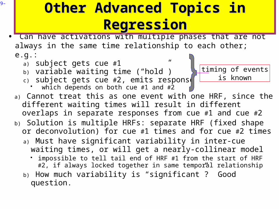
• Can have activations with multiple phases that are not always in the same time relationship to each other; e.g.:

a) subject gets cue #1b) variable waiting time (“hold”)c) subject gets cue #2, emits response

which depends on both cue #1 and #2

a) Cannot treat this as one event with one HRF, since the different waiting times will result in different overlaps in separate responses from cue #1 and cue #2

b) Solution is multiple HRFs: separate HRF (fixed shape or deconvolution) for cue #1 times and for cue #2 timesa) Must have significant variability in inter-cue waiting

times, or will get a nearly-collinear model impossible to tell tail end of HRF #1 from the start of HRF #2, if

always locked together in same temporal relationship

b) How much variability is “significant”? Good question.

Other Advanced Topics in RegressionOther Advanced Topics in Regression

timing of eventsis known

–20–

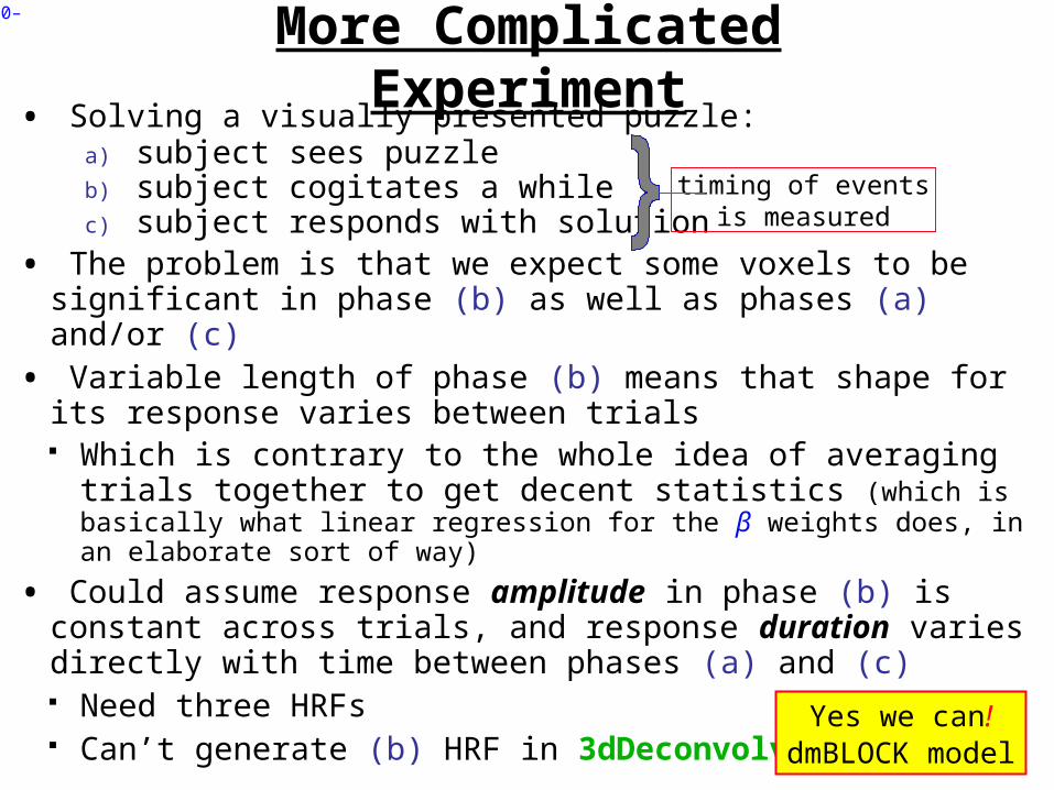
• Solving a visually presented puzzle:a) subject sees puzzleb) subject cogitates a whilec) subject responds with solution

• The problem is that we expect some voxels to be significant in phase (b) as well as phases (a) and/or (c)

• Variable length of phase (b) means that shape for its response varies between trials Which is contrary to the whole idea of averaging trials

together to get decent statistics (which is basically what linear regression for the β weights does, in an elaborate sort of way)

• Could assume response amplitude in phase (b) is constant across trials, and response duration varies directly with time between phases (a) and (c) Need three HRFs Can’t generate (b) HRF in 3dDeconvolve

More Complicated Experiment

timing of eventsis measured

Yes we can!dmBLOCK model

–21–

• When different stimuli in the same class have different (and known) durations

• Controlled by specifying the ‘dmBLOCK’ response model

• Usually used with ‘-stim_times_AM1’ to indicate that an extra parameter is married to each stimulus time Here, parameter is the duration, not amplitude modulation

• You can also use ‘-stim_times_AM2’ , by adding the extra amplitude modulation parameter(s) The duration parameter for ‘dmBLOCK’ is always the last

parameter in a marriage

• For those unfortunates using data that is supplied with FSL-style 3-column stimulus files: “time duration amplitude” You can use ‘-stim_times_FSL’ to process these, without

having to convert them to the AFNI format described herein Which is like using ‘-stim_times_AM1’

Duration Modulation (dm)

–22–

• 3dDeconvolve -nodata 350 1 -polort -1 \ -num_stimts 1 \ -stim_times_AM1 1 q.1D ‘dmBLOCK(1)’ \ -x1D stdout: | 1dplot -stdin -thick –thick

• File q.1D contains 1 line: 10:1 40:2 70:3 100:4 130:5 160:6 190:7 220:8 250:9 280:30

–23–

Noise Issues• “Noise” in FMRI is caused by several factors, not completely characterized MR thermal noise (well understood, unremovable) Cardiac and respiratory cycles (partly understood)

o In principle, could measure these sources of noise separately and then try to regress them out RETROICOR program

Scanner fluctuations (e.g., thermal drift of hardware, timing errors) Small subject head movements (10-100 μm) Very low frequency fluctuations (periods longer than 100 s)

• Data analysis should try to remove what can be removed and should allow for the statistical effects of what can’t be removed “Serial correlation” in the noise time series affects the t- and F-statistics calculated by 3dDeconvolve

Next slides: new AFNI program for dealing with this issue

–24–

• t- and F-statistics denominators: estimates of noise variance White noise estimate of variance:

o N = number of time pointso m = number of fit parameterso N – m = degrees of freedom = how many equal-variance independent

random values are left after time series is fit with m regressors

• ProblemProblem: if noise values at successive time points are correlated, this estimate of variance is biased to be too small, since there aren’t really N – m independent random values left Denominator too small implies t- and F-statistics are too large! And number of degrees of freedom is also too large. So significance (p -value) of activations in individuals is overstated.

• Solution #1Solution #1: estimate correlation structure of noise and then adjust statistics (downwards) appropriately• Solution #2Solution #2: estimate correlation structure of noise and also estimate β fit parameters using more efficient “generalized least squares”, using this correlation, all at once (REML method)

Allowing for Serial CorrelationAllowing for Serial Correlation

–25–

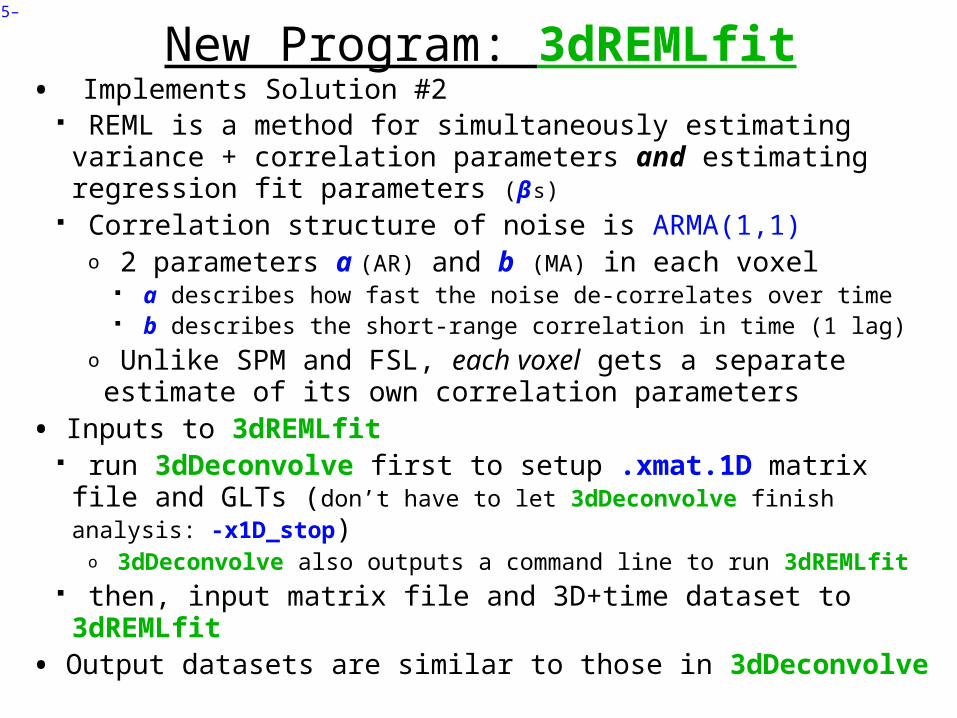
New Program: 3dREMLfit• Implements Solution #2

REML is a method for simultaneously estimating variance + correlation parameters and estimating regression fit parameters (β s)

Correlation structure of noise is ARMA(1,1)o 2 parameters a (AR) and b (MA) in each voxel

a describes how fast the noise de-correlates over time b describes the short-range correlation in time (1 lag)

o Unlike SPM and FSL, each voxel gets a separate estimate of its own correlation parameters

• Inputs to 3dREMLfit run 3dDeconvolve first to setup .xmat.1D matrix file and GLTs (don’t have to let 3dDeconvolve finish analysis: -x1D_stop)

o 3dDeconvolve also outputs a command line to run 3dREMLfit then, input matrix file and 3D+time dataset to 3dREMLfit• Output datasets are similar to those in 3dDeconvolve

–26–

Sample Outputs• Compare with AFNI_data3/afni/rall_regress results• 3dREMLfit -matrix rall_xmat.x1D -input rall_vr+orig -fout -tout \ -Rvar rall_varR -Rbuck rall_funcR -Rfitts rall_fittsR \ -Obuck rall_funcO -Ofitts rall_fittsO

REMLF = 3.15p = 0.001

OLSQF = 3.15p = 0.001

REMLF =1.825p = 0.061 F = No activityoutside brain!

OLSQF =5.358p = 5e-7 F = No activityoutside brain!

Oh

My

GOD!?!

–27–

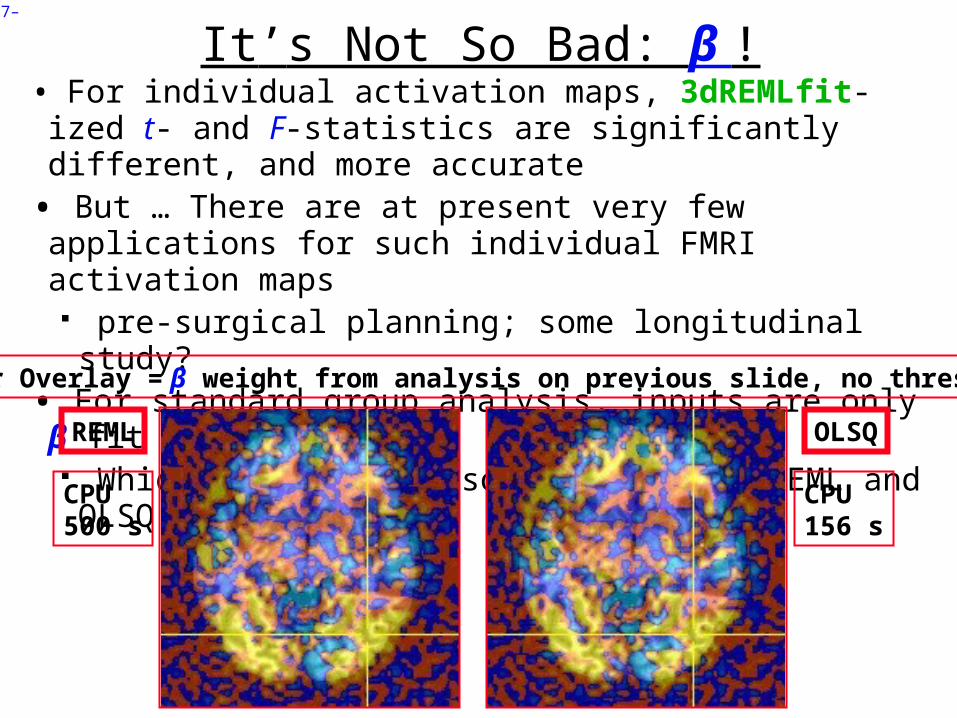
It’s Not So Bad: β !• For individual activation maps, 3dREMLfit-ized t- and F-statistics are significantly different, and more accurate• But … There are at present very few applications for such individual FMRI activation maps pre-surgical planning; some longitudinal study?• For standard group analysis, inputs are only β fit parameters

Which don’t change so much between REML and OLSQ

REML OLSQ

Color Overlay = β weight from analysis on previous slide, no threshold

CPU500 s

CPU156 s

–28–

It’s Not So Bad At All: Group Analysis!• Group analysis activation maps (3dANOVA3) from 16 subjects

REML OLSQ

F -test for Affect condition

F -test for Category condition

F -test for Affect condition

F -test for Category condition

–29–

Nonlinear Regression• Linear models aren’t the only possibility

e.g., could try to fit HRF of the form Unknowns b and c appear nonlinearly in this formula• Program 3dNLfim can do nonlinear regression (including

nonlinear deconvolution) User must provide a C function that computes the model time series, given a set of parameters (e.g., a, b, c)

o We could help you develop this C model functiono Several sample model functions in the AFNI source code distribution

Program then drives this C function repeatedly, searching for the set of parameters that best fit each voxel

Has been used to fit pharmacological wash-in/wash-out models (difference of two exponentials) to FMRI data acquired during pharmacological challenges

o e.g., injection of nicotine, cocaine, ethanol, etc.o these are difficult experiments to do and to analyze

–30–

Deconvolution: The Other Direction• Signal model: Z(t) = H(t)★A(t) + baseline model + noise

• H(t) = HRF = response magnitude t seconds after activation H(t) is causal = zero for t < 0 “★” is symbol for convolution, not multiplication!

• 3dDeconvolve: find out something about H(t) given A(t)

• Sometimes (PPI) want to solve the problem in the other direction: assume a model for H(t) and find time series A(t) Convolution is commutative: H(t)★A(t) = A(t)★H(t) So the other direction looks to be the same problem But isn’t, since H(t) is causal but A(t) is not

o Also, H(t)★A(t) smooths out rough spots in A(t), so undoing this deconvolution adds roughness — including noise, which is already rough — which must be controlled or output A(t) will be junk

• Program 3dTfitter solves this type of problem Also can allow for per voxel baseline model components

–31–

• Smooth data in space before analysis

• Average data across anatomically-selected regions of interest ROI (before or after analysis)

• Labor intensive (i.e., hire more students)

• Or could use ROIs from atlases, or from FreeSurfer per-subject parcellation

• Reject isolated small clusters of above-threshold voxels after analysis

Spatial Models of ActivationSpatial Models of Activation

–32–

Spatial Smoothing of DataSpatial Smoothing of Data• Reduces number of comparisons• Reduces noise (by averaging)

• Reduces spatial resolution• Blur it enough: Can make FMRI results look like

low resolution (1990s) PET data

• Smart smoothing: average only over nearby brain or gray matter voxels• Uses resolution of FMRI cleverly• 3dBlurToFWHM3dBlurToFWHM and and 3dBlurInMask3dBlurInMask

• Or, average over selected ROIs• Or, cortical surface based smoothing

• Estimate smoothness with 3dFWHMx3dFWHMx

–33–

3dBlurToFWHM• Program to smooth FMRI time series datasets to a specified smoothness (as estimated by FWHM of noise spatial correlation function) Don’t just add smoothness (à la 3dmerge) but control it (locally and

globally) Goal: use datasets from diverse scanners

• Why blur FMRI time series? Averaging neighbors will reduce noise Activations are (usually) blob-ish (several voxels across) Diminishes the multiple comparisons problem

• 3dBlurToFWHM and 3dBlurInMask blur only inside a mask region To avoid mixing air (noise-only) and brain voxels Partial Differential Equation (PDE) based blurring method

o 2D (intra-slice) or 3D blurring

–34–

Spatial ClusteringSpatial Clustering• Analyze data, create statistical map

(e.g., t statistic in each voxel)

• Threshold map at a low t value, in each voxel separately• Will have many false positives

• Threshold map by rejecting clusters of voxels below a given size• Can control false-positive rate by

adjusting t (or F) threshold and cluster-size thresholds together: 3dClustSim

–38–

MMuullttii -Voxel Statistics

Spatial Clustering&&

False Discovery Rate:

“Correcting” the Significance

–39–

Basic Problem

• Usually have 50-200K FMRI voxels in the brain

• Have to make at least one decision about each one: Is it “active”?

o That is, does its time series match the temporal pattern of activity we expect?

Is it differentially active?o That is, is the BOLD signal change in task #1 different from task #2?

• Statistical analysis is designed to control the error rate of these decisions Making lots of decisions: hard to get perfection in statistical testing

–41–

• Family-Wise Error (FWE) Multiple testing problem: voxel-wise statistical analysis

o With N voxels, what is the chance to make a false positive error (Type I) in one or more voxels?

Family-Wise Error: αFW = 1–(1–p)N →1 as N increases

o For Np small (compared to 1), αFW ≈ Np

o N ≈ 50,000+ voxels in the brain

o To keep probability of even one false positive αFW < 0.05 (the

“corrected” p-value), need to have p < 0.05 / 5×104 = 10–6

o This constraint on the per-voxel (“uncorrected”) p-value is so stringent that we would end up rejecting a lot of true positives (Type II errors) also, just to be safe on the Type I error rate

• Multiple testing problem in FMRI 3 occurrences of multiple tests: Individual, Group, and Conjunction Group analysis is the most severe situation (have the least data,

considered as number of independent samples = subjects)

–42–

• Two Approaches to the “Curse of Multiple Comparisons” Control FWE to keep expected total number of false positives below 1

o Overall significance: αFW = Prob(≥ one false positive voxel in the whole brain)

o Bonferroni correction: αFW = 1– (1–p)N ≈ Np, if p << N –1

Use p = α /N as individual voxel significance level to achieve αFW = α Too stringent and overly conservative: p = 10–8…10–6

o What can rescue us from this hell of statistical super-conservatism? Correlation: Voxels in the brain are not independent

Especially after we smooth them together! Means that Bonferroni correction is way way too stringent

Contiguity: Structures in the brain activation map We are looking for activated “blobs”: the chance that pure noise (H0) will

give a set of seemingly-activated voxels next to each other is lower than getting false positives that are scattered around far apart

Control FWE based on spatial correlation (smoothness of image noise) and minimum cluster size we are willing to accept

Control false discovery rate (FDR) — Much more on this a little later!o FDR = expected proportion of false positive voxels among all detected voxels

Give up on the idea of having (almost) no false positives at all

–43–

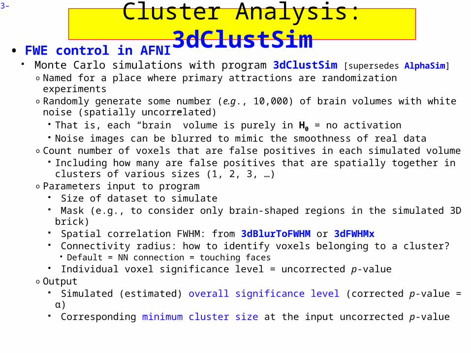
• FWE control in AFNI Monte Carlo simulations with program 3dClustSim [supersedes AlphaSim]

o Named for a place where primary attractions are randomization experiments o Randomly generate some number (e.g., 10,000) of brain volumes with white

noise (spatially uncorrelated) That is, each “brain” volume is purely in H0 = no activation Noise images can be blurred to mimic the smoothness of real data

o Count number of voxels that are false positives in each simulated volume Including how many are false positives that are spatially together in clusters

of various sizes (1, 2, 3, …)o Parameters input to program

Size of dataset to simulate Mask (e.g., to consider only brain-shaped regions in the simulated 3D brick) Spatial correlation FWHM: from 3dBlurToFWHM or 3dFWHMx Connectivity radius: how to identify voxels belonging to a cluster?

Default = NN connection = touching faces Individual voxel significance level = uncorrected p-value

o Output Simulated (estimated) overall significance level (corrected p-value = α) Corresponding minimum cluster size at the input uncorrected p-value

Cluster Analysis: 3dClustSim

–44–

• Example: 3dClustSim -nxyz 64 64 30 -dxyz 3 3 3 -fwhm 7

p-value ofthreshold

# 3dClustSim -nxyz 64 64 30 -dxyz 3 3 3 -fwhm 7 # Grid: 64x64x30 3.00x3.00x3.00 mm^3 (122880 voxels)

# CLUSTER SIZE THRESHOLD(pthr,alpha) in Voxels # -NN 1 | alpha = Prob(Cluster >= given size)

# pthr | 0.100 0.050 0.020 0.010# ------ | ------ ------ ------ ------ 0.020000 89.4 99.9 114.0 123.0 0.010000 56.1 62.1 70.5 76.6 0.005000 38.4 43.3 49.4 53.6 0.002000 25.6 28.8 33.3 37.0 0.001000 19.7 22.2 26.0 28.6 0.000500 15.5 17.6 20.5 22.9 0.000200 11.5 13.2 16.0 17.7 0.000100 9.3 10.9 13.0 14.8

At a per-voxel p=0.005, a cluster should have 44+ voxels to occur with α < 0.05 from noise only

3dClustSim can be run by afni_proc.py : results get storedinto statistics dataset, and then used in AFNI Clusterize GUI

–45–

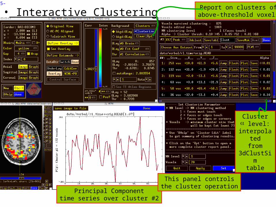
• Interactive Clustering

Principal Componenttime series over cluster #2

This panel controlsthe cluster operation

Report on clusters ofabove-threshold voxels

Cluster level:

interpolatedfrom

3dClustSimtable

False Discovery Rate in • Situation: making many statistical tests at once

e.g, Image voxels in FMRI; associating genes with disease

• Want to set threshold on statistic (e.g., F- or t-value) to control false positive error rate

• Traditionally: set threshold to control probability of making a single false positive detection But if we are doing 1000s (or more) of tests at once, we

have to be very stringent to keep this probability low

• FDR: accept the fact that there will be multiple erroneous detections when making lots of decisions Control the fraction of positive detections that are wrong

o Of course, no way to tell which individual detections are right!

Or at least: control the expected value of this fraction

–46–

FDR: q [and z(q)]• Given some collection of statistics (say, F-values from 3dDeconvolve), set a threshold h

• The uncorrected p-value of h is the probability that F > h when the null hypothesis is true (no activation) “Uncorrected” means “per-voxel” The “corrected” p-value is the probability that any voxel is

above threshold in the case that they are all unactivated If have N voxels to test, pcorrected = 1–(1–p)N ≈ Np (for small p)

o Bonferroni: to keep pcorrected< 0.05, need p < 0.05 / N, which is very tiny

• The FDR q-value of h is the fraction of false positives expected when we set the threshold to h Smaller q is “better” (more stringent = fewer false detections)

z(q) = conversion of q to Gaussian z: e.g, z(0.05)≈1.95996

o So that larger is “better” (in the same sense) e.g, z(0.01)≈2.57583

–47–

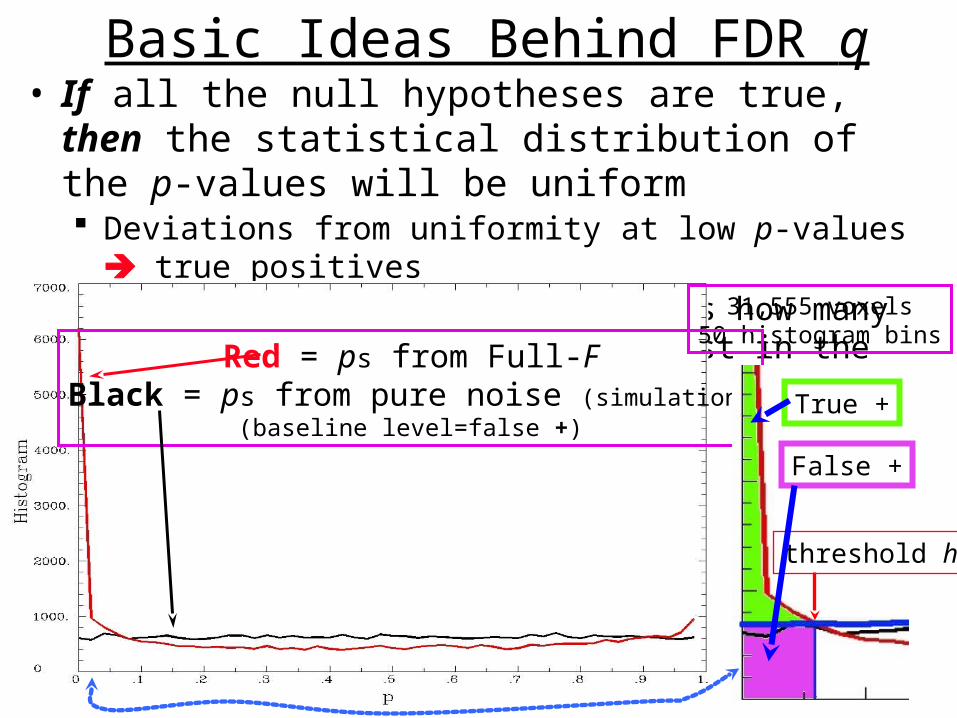
Basic Ideas Behind FDR q• If all the null hypotheses are true, then the statistical

distribution of the p-values will be uniform Deviations from uniformity at low p-values true positives Baseline of uniformity indicates how many true negatives

are hidden amongst in the low p-value region31,555 voxels

50 histogram binsRed = ps from Full-F

Black = ps from pure noise (simulation)(baseline level=false +)

True +

False +

threshold h

Graphical Calculation of q• Graph sorted p-values of voxel #k vs. ζ=k / N (the cumulative histogram of p,

flipped sideways) and draw some lines from origin

Slope=0.10

q=0.10 cutoff

Real data: F-statistics from 3dDeconvolve

Ideal sorted p if notrue positives at all(uniform distribution)

Very small p = very significant

N.B.: q-values depend on data in all voxels,unlike voxel-wise

(uncorrected) p-values!

–50–

FDR curves: h vs. z(q)• 3dDeconvolve, 3dANOVAx, 3dttest, and 3dNLfim now compute FDR curves for all statistical sub-bricks and store them in output header

• 3drefit -addFDR does same for other datasets

3drefit -unFDR can be used to delete such info

• AFNI now shows p- and q-values below the threshold slider bar

• Interpolates FDR curve from header (thresholdzq)

• Can be used to adjust threshold by “eyeball”

–54–

q = N/A means it’s not available MDF hint = “missed detection fraction”

FDR Statistical Issues• FDR is conservative (q-values are too large) when voxels

are positively correlated (e.g., from spatially smoothing) Correcting for this is not so easy, since q depends on data

(including true positives), so a simulation like 3dClustSim is hard to conceptualize

At present, FDR is an alternative way of controlling false positives, vs. 3dClustSim (clustering)

o Thinking about how to combine FDR and clustering

• Accuracy of FDR calculation depends on p-values being uniformly distributed under the null hypothesis Statistic-to-p conversion should be accurate, which means

that null F-distribution (say) should be correctly estimated Serial correlation in FMRI time series means that 3dDeconvolve denominator DOF is too large

p-values will be too small, so q-values will be too smallo3dREMLfit rides to the rescue!

–55–

–56–

• These 2 methods control Type I error in different senses FWE: αFW = Prob (≥ one false positive voxel/cluster in the whole brain)

Frequentist’s perspective: Probability among many hypothetical activation maps gathered under identical conditions

Advantage: can directly incorporate smoothness into estimate of αFW

FDR = expected fraction of false positive voxels among all detected voxels Focus: controlling false positives among detected voxels in one activation map, as

given by the experiment at hand Advantage: not afraid of making a few Type I errors in a large field of true positives

Concrete example Individual voxel p = 0.001 for a brain of 50,000 EPI voxels Uncorrected → ≈ 50 false positive voxels in the brain FWE: corrected p = 0.05 → ≈5% of the time would expect one or more purely false

positive clusters in the entire volume of interest FDR: q = 0.05 → ≈5% of voxels among those positively labeled ones are false positive

•What if your favorite blob (activation area) fails to survive correction? Tricks (don’t tell anyone we told you about these)

One-tail t -test? NN=3 clustering? ROI-based statistics – e.g., grey matter mask, or whatever regions you focus on

Analysis on surface; or, Use better group analysis tool (3dLME, 3dMEMA, etc.)

FWE or FDR?

–57–

•Conjunction Dictionary: “a compound proposition that is true if and only if all of its

component propositions are true” FMRI: areas that are active under 2 or more conditions (AND logic)

o e.g, in a visual language task and in an auditory language task In FMRI papers: Is also be used to mean analysis to find areas that are

exclusively activated in one task but not another (XOR logic) or areas that are active in either task (non-exclusive OR logic)

If have n different tasks, have 2n possible combinations of activation overlaps in each voxel (ranging from nothing there to complete overlap)

Tool: 3dcalc applied to statistical mapso Heaviside step function defines a On / Off logico step(t-a) = 0 if t < a = 1 if t > ao Can be used to apply more than one

threshold at a time

Conjunction Analysis

a

–58–

• Example of forming all possible conjunctions 3 contrasts/tasks A, B, and C, each with a t-stat from 3dDeconvolve Assign each a number, based on binary positional notation:

o A: 0012 = 20 = 1 ; B: 0102 = 21 = 2 ; C: 1002 = 22 = 4 Create a mask using 3 sub-bricks of t (e.g., threshold = 4.2) 3dcalc -a ContrA+tlrc -b ContrB+tlrc -c ContrC+tlrc \

-expr '1*step(a-4.2)+2*step(b-4.2)+4*step(c-4.2)' \

-prefix ConjAna Interpret output, which has 8 possible (=23) scenarios: 0002 = 0: none are active at this voxel

0012 = 1: A is active, but no others

0102 = 2: B, but no others

0112 = 3: A and B, but not C

1002 = 4: C but no others

1012 = 5: A and C, but not B

1102 = 6: B and C, but not A

1112 = 7: A, B, and C are all active at this voxel

Can display each

combination with a

different color and so make pretty pictures that might even

mean something!

–59–

• Multiple testing correction issue How to calculate the p-value for the conjunction map? No problem, if each entity was corrected (e.g., cluster-size

thresholded at t =4.2) before conjunction analysis, via 3dClustSim

But that may be too stringent (conservative) and over-corrected

With 2 or 3 entities, analytical calculation of conjunction pconj

is possible Each individual test can have different uncorrected (per-voxel) p Double or triple integral of tails of non-spherical (correlated) Gaussian

distributions — not available in simple analytical formulae

With more than 3 entities, may have to resort to simulations Monte Carlo simulations? (AKA: Buy a fast computer) Will Gang Chen write such a program? Only time will tell!