1. 2. government accession no. - som - state of michigan mdot form no. technical report...
TRANSCRIPT

; MDOT Form No. Technical Report Documentation Pa~e 1. Report No. 2. Government Accession No. 3. MDOT Project Manager
R-1519 4. Title and Subtitle 5. Report Date
Calculating the Critical Buckling Stress for Plates with September 2008 One Free Edge Under Combined Axial and Flexural 6. Performing Organization Code Forces
7. Autbor(s) 8. Performing Org. Report No. Rebecca Curtis, P.E., and Roger Till, P.E.
9. Performing Organization Name and Address 10. Work Unit No. (TRAlS) Michigan Department of Transportation Construction and Technology Division 11. Contract No. P.O. Box 30049 Lansing, Ml 48909
ll(a). Authorization No.
12. Sponsoring Agency Name and Address 13. Type of Report & Period Covered
Michigan Department of Transportation Final Report, 7/08-9/08 Constrution and Technology Division P.O. Box 30049 14. Sponsoring Agency Code Lansing, Ml 48909
15. Supplementary Notes
16. Abstract
Analysis of gusset plates in truss structures may include checking the combined axial and flexural stresses in a section of the plate. Using concentrically loaded column equations for this analysis provides overly conservative results and may suggest that unnecessary repairs are required. Gusset plates may be treated as plates with the loaded edges supported and the unloaded edges having one edge supported and one edge free. In the review of the literature, formulas and/or buckling coefficients were available for many combinations of plate loading and restraint, but did not include the specific case needed for assessment of gusset plates. Using the energy method and the work of Timoshenko, and Lindquist and Stowell as a basis, equations were developed to find the critical buckling stress for a plate having simply supported loaded edges, a simply supported unloaded edge and a free loaded edge. The equations developed are applicable to rectangular plates with any length to width ratio and also to any combination of linear-varying stress.
17.KeyWords 18. Distribution Statement
critical buckling stress, gusset plate, free edge, No restrictions. This document is
combined axial and flexural stress available to the public through the Michigan Department of Transportation.
19. Security Classification- report 20. Security Classification- page 21. No. of Pages 22. Price Unclassified Unclassified 27


MICHIGAN DEPARTMENT OF TRANSPORTATION MDOT
Calculating the Critical Buckling Stress for Plates with One
Free Edge Under Combined Axial and Flexural Forces
Rebecca Curtis, P.E., and Roger Till, P.E.
Structural Section Construction and Technology Division
Research Report R-1519
Michigan Transportation Commission Ted B. Wahby, Chairman
Linda Miller Atkinson, Vice Chairwoman Maureen Miller Brosnan, Jerrold Jung
Steven K. Girard, James S. Scalici Kirk T. Steudle, Director
Lansing, Michigan September 2008

The information contained in this report was compiled exclusively for the use of the Michigan Department of Transportation. Recommendations contained herein are based upon the research data obtained and the expertise of the researchers, and are not necessarily to be construed as Department policy. No material contained herein is to be reproduced-wholly or in part-without the expressed permission of the Engineer of Construction and Technology.
ii

TABLE OF CONTENTS Background.................................................................................................................................... 1 Energy Method............................................................................................................................... 2 Comparison of Energy Method to Tabulated Values .................................................................... 9 Comparison of Energy Method to Finite Element Values............................................................. 9 Comparison of Energy Method to Finite Element Values for Sample Gusset Plate ................... 10 Resistance Factors........................................................................................................................ 14 Summary ...................................................................................................................................... 15 References.................................................................................................................................... 17 Appendices................................................................................................................................... 18
iii


BACKGROUND When checking gusset plates at sections other than at the point of intersection of the chords, eccentricity of the forces may introduce bending forces in the plate. The width of the section tends to be longer than the unbraced length, and so a small eccentricity may produce compressive bending stresses equal to or greater than the pure axial loading. Due to concern over buckling under compression, these combined effects should be evaluated. While evaluating the tragic collapse of I-35W in Minnesota, these combined forces were evaluated by Holt (1) in the Federal Highway Administration (FHWA) Turner-Fairbanks Highway Research Center Report against:
2
*56.0000,22 ⎟⎠⎞
⎜⎝⎛−
rLpsi Eq. 1
where L is the unsupported length and r is the radius of gyration of the member, both in inches. This equation is related to the buckling stress of a column. In contrast to this, the FHWA Bridge Design Guidance No. 1, Load Rating Evaluation of Gusset Plates in Truss Bridges, Parts A and B (2), suggested, in a draft version, that combined axial and bending forces should be evaluated against fy, the yield strength of the material. Upon further investigation, the FHWA Bridge Design Guidance No. 1 was modified to state that gusset plates act as deep members and this check is not required. While it will be shown that the proposed method is conservative, the authors of this report feel that this check will provide assurance to bridge owners that the intent of the historic criteria (see Eq. 1 above) is being met. Upon inspection, a number of differences can be found between the case of a concentrically loaded column and the free body diagram of a gusset plate. In the case of a column, a four sided plate is loaded at opposing edges. These edges may be simple or fixed, and are assumed to be loaded uniformly in compression. The perpendicular edges are free, or unsupported. The stiffness of the plate is generally also uniform across the section. Finally, multiple modes of buckling may form in the column dependent upon the geometric properties of the section. In contrast to the properties of a column discussed above, the section of a gusset plate is not similar to a column. The four sided section is loaded at opposing edges, which may be simple or fixed, but the loading is not uniform due to the eccentric loading. One perpendicular edge is free, however the other edge may be fixed, simple, or some case in-between due to the connections with the truss members. The stiffness of the plate is not uniform, as triangular unbraced areas are formed between the truss members. The stiffness increases as the unbraced length decreases, and these areas retard the buckling of the extreme fiber. Finally, as there is only one free edge, the mode of buckling is critical at one half wave, as will be discussed. While current AASHTO bridge codes provide an equation for the combined axial and bending (or eccentric loading) of a column, this does not take into account that one of the unloaded edges is retrained. Additionally, the moment capacity of a plate with an unsupported compression edge is not defined in the AASHTO bridge codes. It is assumed that a reduction in moment capacity from beam theory, or yield stress times the section modulus, would be required to account for the
1

unbraced compression edge. Finally, the AASHTO codes are based upon rolled section with residual compression stresses at the free edges. Contrary to this, plates with flame cut edges have tensile residual stresses at the edge (3). ENERGY METHOD In order to analyze the special case of a gusset plate under combined axial and flexural loads, we returned to plate buckling theory. In a paper by Lundquist and Stowell (4), the energy method is used to determine the critical buckling stress of a plate under uniform compression with varying levels of edge restraint (from fixed to simple) of one unloaded edge. The opposite unloaded edge is free. Loaded edges are simply supported. The critical stress is obtained from the condition of neutral stability: T=V1+V2 Eq. 2 Where T is the energy from the loading, V1 is the energy of the plate resisting the load and V2 is the energy of the restraining edge resisting the load. For our case, in order to be conservative, we are assuming that the restraining edge is simple and does not contribute to the resisting energy. Therefore, V2=0 and Equation 2 simplifies to: T=V1 Eq. 3 Lundquist and Stowell (4) further define the energies as:
∫ ∫−
⎟⎠⎞
⎜⎝⎛
∂∂
=b
dydxxwtfT
0
2
2
2
****21
λ
λ
Eq. 4
And
∫ ∫− ⎪⎭
⎪⎬⎫
⎪⎩
⎪⎨⎧
⎥⎥⎦
⎤
⎢⎢⎣
⎡
∂∂
∂∂
−⎟⎟⎠
⎞⎜⎜⎝
⎛∂∂
∂−+⎟⎟
⎠
⎞⎜⎜⎝
⎛∂∂
+∂∂
=b
dydxyw
xw
yxw
xw
xwDV
0
2
2
2
2
2
2222
2
2
2
2
1 ****)1(*2*2
λ
λ
υ Eq. 5
Where: w is the deflection perpendicular to the plane of the plate
( )2
3
1*12*
υ−=
tED and is the flexural rigidity of the plate
f is the compressive force t is the thickness of the plate λ is the length of the half wave
2

υ is Poisson’s ratio of the material and a, b, x and y are as shown in Figure 1.
Figure 1: Plate with three restrained edges and one free edge under compressive loading
In a series of steps in Lundquist and Stowell (4) the deflection equation is found as:
⎟⎠⎞
⎜⎝⎛
⎪⎭
⎪⎬⎫
⎪⎩
⎪⎨⎧
⎥⎥⎦
⎤
⎢⎢⎣
⎡⎟⎠⎞
⎜⎝⎛+⎟
⎠⎞
⎜⎝⎛+⎟
⎠⎞
⎜⎝⎛+⎟
⎠⎞
⎜⎝⎛+=
λπε x
bya
bya
bya
by
abyAw *cos*****
2*
2
3
3
2
4
1
5
3
Eq. 6
where a1, a2 and a3 are constants that help to describe the shape caused by the restraint coefficient ε. As we are assuming the edge to conservatively be simply supported, ε=0 and these terms drop out, leaving:
⎟⎠⎞
⎜⎝⎛
⎟⎠⎞
⎜⎝⎛=
λπ x
byAw *cos** Eq. 7
In evaluating this equation, Timoshenko (5) found that the smallest buckling stress is when there was only one half-wave, or λ = 1*a. This implies that the plate will only buckle in this one mode, as the critical stress is first reached in this shape. Substituting this value into Eq. 7 we are able to find the required derivatives of the deflection equation.
⎟⎠⎞
⎜⎝⎛
⎟⎠⎞
⎜⎝⎛=
ax
byAw *cos** π
⎟⎠⎞
⎜⎝⎛−=
∂∂
ax
bayA
xw *sin*
*** ππ Eq. 8
3

⎟⎠⎞
⎜⎝⎛−=
∂∂
ax
bayA
xw *cos*
***
2
22 ππ Eq. 9
⎟⎠⎞
⎜⎝⎛=
∂∂
ax
bA
yw *cos* π
02
2
=∂∂
yw Eq. 10
⎟⎠⎞
⎜⎝⎛−=
∂∂∂
ax
baA
yxw *sin*
**2 ππ Eq. 11
Timoshenko (5) also evaluated a case with variable loading and all sides of the plate simply supported. In this case, the deflected shape did not change as compared to the uniformly loaded case, but the force, f, in T (Eq.4) changed from a constant to an equation based on y. Figure 2 identifies the loading situations considered for the gusset plate.
4

Figure 2: Loading cases for plate simply supported at y=0 and free at y=b
In Figure 2, σb is the bending stress and σc is the pure axial stress. A discontinuity occurs when σc=0, and so a different equation will be created for this case. In the case that there is a compressive force, the force equation can be represented as:
( ) Cymyf += * Eq. 12 Examining Figure 2 and solving at known points of f(0) and f(b) we find the values of m and C.
NA
bbc
Cforsolving
NA
bbc y
bCCmy
bf *0**)0( __ σσσσσσ −+=⎯⎯⎯⎯⎯ →⎯+=−+= Eq. 13
5

NA
bmforsolving
NA
bbcbc y
my
bbmbf σσσσσσ =⎯⎯⎯⎯⎯ →⎯−++=+= __**)( Eq. 14
Combining Eqs 13 and 14 it follows that,
( bymC NAc −+= * )σ Eq. 15 The force equation then becomes:
( )NA
bbc
NA
b
yb
yy
yf*
*σ
σσσ
−++= Eq. 16
where yNA is the distance (a constant) from the free edge to the neutral axis of the bending force. Substituting Eqs. 8 and 16 into Eq. 4 and then solving the double integral we find:
( )∫ ∫−
⎥⎦
⎤⎢⎣
⎡⎟⎠⎞
⎜⎝⎛−+=
b
dydxa
xba
yAtCymT0
2
2
2
**sin**
******21
λ
λ
ππ
( )∫ ∫−
⎥⎦
⎤⎢⎣
⎡⎟⎠⎞
⎜⎝⎛+=
b
dydxa
xba
yACymtT0
2
2
222
222
**sin**
*****2
λ
λ
ππ
( )∫ ∫−
⎟⎠⎞
⎜⎝⎛+=
b
dydxa
xyCymba
AtT0
2
2
2222
22
**sin******2**
λ
λ
ππ
( )2
20
222
22 **2sin*42
******2**
a
a
b
dya
xaxyCymba
AtT−
∫ ⎥⎦
⎤⎢⎣
⎡⎟⎠⎞
⎜⎝⎛−+=
ππ
π
( )∫⎭⎬⎫
⎩⎨⎧
⎥⎦
⎤⎢⎣
⎡⎟⎠⎞
⎜⎝⎛ −
−−
−⎥⎦
⎤⎢⎣
⎡⎟⎠⎞
⎜⎝⎛−+=
b
dya
aaaa
aaayCymba
AtT0
222
22
2***2sin*
42*22***2sin*
42*2****
**2** π
ππ
ππ
( )∫ +=b
dyayCymba
AtT0
222
22
2****
**2** π
6
byCym
baAtT
0
34
2
22
3*
4**
**4**
⎟⎟⎠
⎞⎜⎜⎝
⎛+=
π
⎥⎦
⎤⎢⎣
⎡⎟⎟⎠
⎞⎜⎜⎝
⎛+−⎟⎟
⎠
⎞⎜⎜⎝
⎛+=
30*
40*
3*
4**
**4** 3434
2
22 CmbCbmba
AtT π
⎥⎦
⎤⎢⎣
⎡⎟⎟⎠
⎞⎜⎜⎝
⎛+=
3*
4**
*4** 222 bCbma
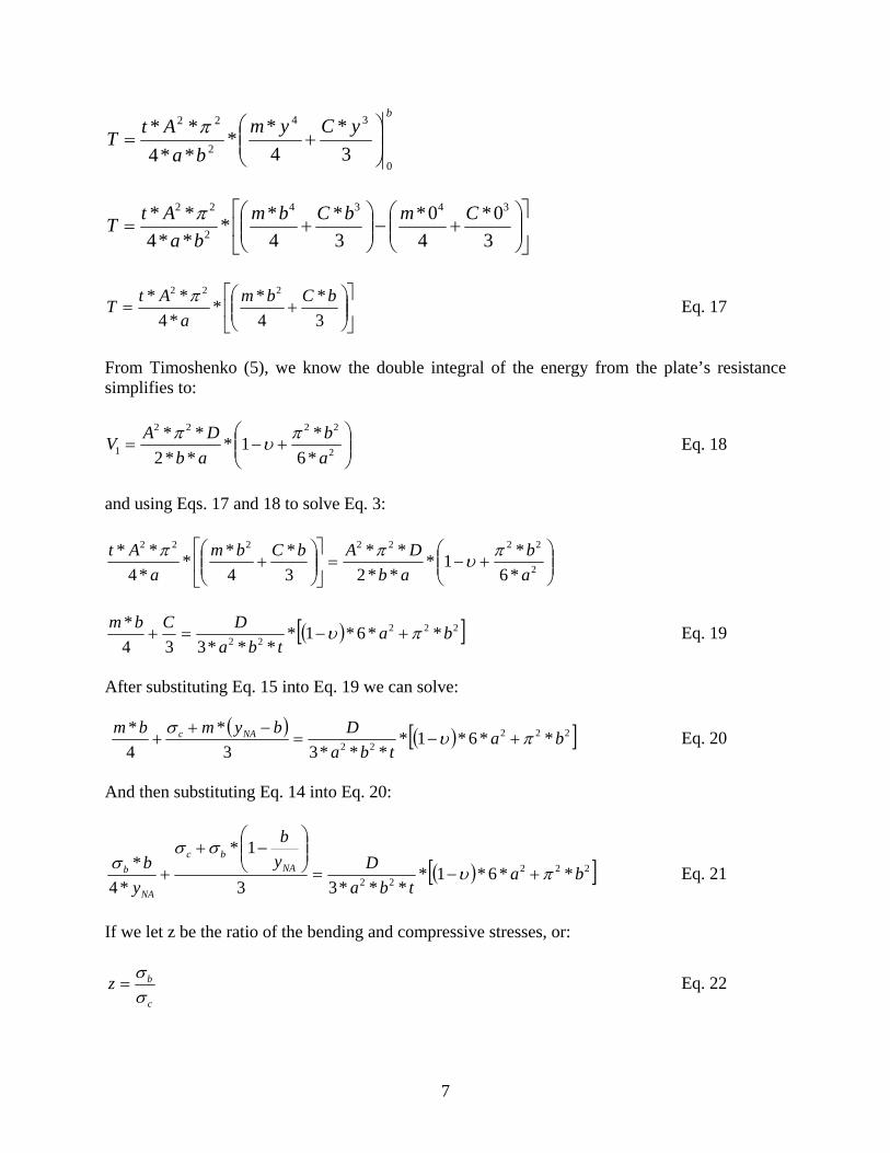
AtT π Eq. 17
From Timoshenko (5), we know the double integral of the energy from the plate’s resistance simplifies to:
⎟⎟⎠
⎞⎜⎜⎝
⎛+−= 2
2222
1 *6*1*
**2**
ab
abDAV πυπ Eq. 18
and using Eqs. 17 and 18 to solve Eq. 3:
⎟⎟⎠
⎞⎜⎜⎝
⎛+−=⎥
⎦
⎤⎢⎣
⎡⎟⎟⎠
⎞⎜⎜⎝
⎛+ 2
2222222
*6*1*
**2**
3*
4**
*4**
ab
abDAbCbm
aAt πυππ
( )[ 22222 **6*1*
***334* ba
tbaDCbm πυ +−=+ ] Eq. 19
After substituting Eq. 15 into Eq. 19 we can solve:
( ) ( )[ ]22222 **6*1*
***33*
4* ba
tbaDbymbm NAc πυσ
+−=−+
+ Eq. 20
And then substituting Eq. 14 into Eq. 20:
( )[ 22222 **6*1*
***33
1*
*4* ba
tbaDy
b
yb NA
bc
NA
b πυσσ
σ+−=
⎟⎟⎠
⎞⎜⎜⎝
⎛−+
+ ] Eq. 21
If we let z be the ratio of the bending and compressive stresses, or:
c
bzσσ
= Eq. 22
7

then we can solve for σc,:
( )[ ]22222 **6*1*
***33
1**
*4** ba
tbaDy
bz
ybz NA
cc
NA
c πυσσ
σ+−=
⎟⎟⎠
⎞⎜⎜⎝
⎛−+
+
( )[ ]22222 **6*1*
***33
1*1
*4* ba
tbaDy
bz
ybz NA
NAc πυσ +−=
⎥⎥⎥⎥⎥
⎦
⎤
⎢⎢⎢⎢⎢
⎣
⎡⎟⎟⎠
⎞⎜⎜⎝
⎛−+
+
( )[ ]
⎥⎥⎥⎥⎥
⎦
⎤
⎢⎢⎢⎢⎢
⎣
⎡⎟⎟⎠
⎞⎜⎜⎝
⎛−+
+
+−=
3
1*1
*4*
**6*1****3
22222
NA
NA
c
ybz
ybz
batba
D πυσ Eq. 23
Once the compressive stress is found, the total stress can be found by:
( zccrit += 1* )σσ Eq. 24 If the compressive stress is zero, then z cannot be found using Eq. 24. For the case where the plate is in pure bending, Eq. 21 can be simplified as:
( )[ ]22222 **6*1*
***33
10
*4* ba
tbaDy
b
yb NA
NAb πυσ +−=
⎟⎟⎟⎟⎟
⎠
⎞
⎜⎜⎜⎜⎜
⎝
⎛⎟⎟⎠
⎞⎜⎜⎝
⎛−+
+
( )[ ]
3
1
*4
**6*1****3
22222
⎟⎟⎠
⎞⎜⎜⎝
⎛−
+
+−==
NA
NA
critb
yb
yb
batba
D πυσσ Eq. 25
As can be seen, the critical stress is dependent upon the ratio of the compressive and bending forces, the geometry of the plate and the modulus and poisson’s ratio of the material. Given
8

these inputs, the critical buckling stress can be found analytically. In order to compare to tabulated values, the k factor, or buckling coefficient, can be found from the critical stress as:
( )22
22
***1*12*
tEbk crit
πυσ −
= Eq. 26
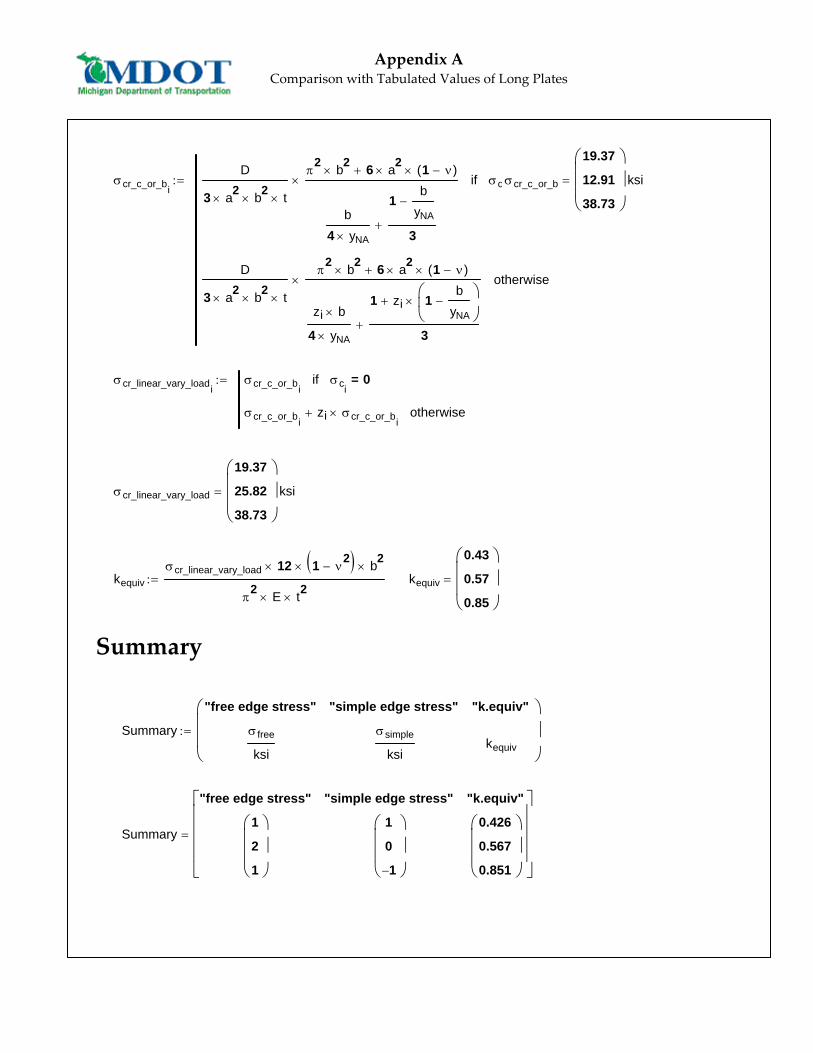
COMPARISON OF ENERGY METHOD TO TABULATED VALUES Values for the minimum buckling coefficient, k, have been tabulated by Johnston (6). These factors are related to the ratio of the compressive and bending stresses, and do not take into account the geometry of the plate, as do Eqs. 23 and 25. However, if we use a long plate in Eqs. 23 and 25 and assume a few material properties the calculated buckling coefficient can be compared with the tabulated values and are shown in Table 1. The calculations are shown in Appendix A.
200=ba
3.0=υ
2byNA =
Table 1: Long Plate Minimum Buckling Coefficients, k
Long Plate Minimum Buckling Coefficients, k
Z Tabulated
Value Calculated
Value 0 pure compression 0.42 0.426 1 σc = σb, max comp. stress at free edge 0.57 0.567 ∞ pure bending 0.85 0.851
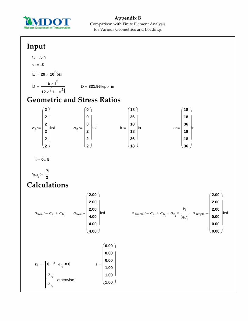
COMPARISON OF ENERGY METHOD TO FINITE ELEMENT VALUES As the tabulated values only cover long, rectangular plate geometries, Finite Element Analyses (FEA) were performed to further evaluate the accuracy of the energy method. The program GTStrudl was used to create the models. Known solutions of classical buckling theory were used to verify the elastic buckling FEA models prior to applying it to these cases. Various ratios of loading and geometry were analyzed. GTStrudl generated a non-dimensional buckling multiplier, buck, (not to be confused with k, the buckling coefficient), which could then be converted into a buckling stress.
max*σσ buckcrit = Eq. 27
9

The buckling stress from GTStrudl is compared with the critical buckling stress found using the Energy Method in Table 2. The Energy Method calculations are shown in Appendix B.
Table 2: FEA Model versus Energy Method for various geometric and loading ratios Plate
Dimensions Loading Values at edge FEA Model Energy Method Difference
a (in) b (in) Simple (ksi) Free (ksi) Buckling Multiplier σcr (ksi) σcr (ksi) %
18 18 2.0 2.0 14.19 28.38 28.83 -1.56% 18 36 2.0 2.0 10.97 21.94 22.36 -1.88% 36 18 2.0 2.0 6.76 13.52 13.66 -1.02% 18 18 0.0 4.0 9.46 37.84 38.44 -1.56% 18 36 0.0 4.0 7.07 28.28 29.83 -5.20% 36 18 0.0 4.0 4.52 18.08 18.22 -0.77%
COMPARISON OF ENERGY METHOD TO FINITE ELEMENT VALUES FOR SAMPLE GUSSET PLATE The Energy Method formulas are based upon a rectangular section. In the truss gusset plates that drive the need for this analysis method, the actual section in combined bending and axial forces is triangular in shape. The unbraced length, a, is taken at the free edge. The loaded edge, b, is taken to be the distance from the loaded edge to the joint center. A sample gusset plate was analyzed using the Energy Method and also by FEA. It is not assumed that the values will be the same, as the stiffness of the plate itself will decrease from the simple edge to the free edge (as y goes from 0 to b). However, it is assumed that the Energy Method will be conservative as the smallest stiffness will be applied to the entire plate.
10

Figure 3: Chord loading on sample gusset plate
The sample ½ inch gusset plate is shown in Figure 3. The factored loading of the chords is also shown. The gusset plate was digitized from shop drawings to generate the dimensions. In order to apply the Energy Method, sections were chosen. For this example, the sections were taken at the top edge of the bottom chord (Section 1) and at the right edge of the vertical (Section 2). The factored axial compressive stresses were found at these two sections as well as the factored bending stresses. The axial and bending stresses were combined at the edge of the section (the free edge) and at the point where the plate is assumed to be simply supported. For Section 1, the plate was assumed to be simply supported at the extension of the joint center. For Section 2, the plate was assumed to be simply supported at the edge of the horizontal chord. Dimension a was found as the length of the free edge and b is the distance from the free edge to the assumed point of simple support. Figure 4 demonstrates how these distances were measured for the sample gusset plate.
11

Figure 4: Measured distances for Sections 1 and 2 of a sample gusset plate
Using the stresses and plate dimensions found from the sample gusset plate, idealized rectangular sections were analyzed according to Eqs. 24 and 25. Table 3 documents the Energy Method and FEA for the idealized gusset plates. The idealized gusset plate Energy Method calculations are given in Appendix C.
Table 3: FEA Model versus Energy Method for sample gusset plate Plate Dimensions
Loading Values at edge FEA Model Energy
Method Difference Section Location
a (in) b (in) Simple (ksi)
Free (ksi)
Buckling Multiplier σcr (ksi) σcr (ksi) %
Section 1 36.7 45.0 2.0 3.5 1.97 6.90 6.99 -1.36% Section 2 13.0 34.5 11.8 27.1 1.70 46.07 47.87 -3.76%
In addition, the entire gusset plate was modeled, rather than the sections that have been analyzed as idealized rectangles. Gusset plate thicknesses were increased in the areas overlapping with chord members, as indicated by the darker areas in Figure 3, to reflect the increased stiffness provided by the chord members. Loading on the gusset plate was through all the nodes in contact with the chord members, as shown in Figure 5.
12

Figure 5: Regions of loading for sample gusset plate FEA model
The buckling coefficient of the entire gusset plate for the calculated loads was much higher than the coefficient calculated for a particular rectangular section. An iterative process was used that reduced the stiffness of the portions of the gusset plate at yield until changing the stiffness had little effect on the buckling multiplier. The FEA buckling multiplier for the gusset plate was 6.27, demonstrating the conservatism of the Energy Method (see Table 3 where the buckling multiplier calculated was near 2) and the reserve safety. Figure 6 shows the anticipated buckled shape of the entire gusset plate from the FEA model. The plate has been rotated to best show the buckling. Figure 7 shows the minimum principle stress contours for the final iteration of stiffness.
13
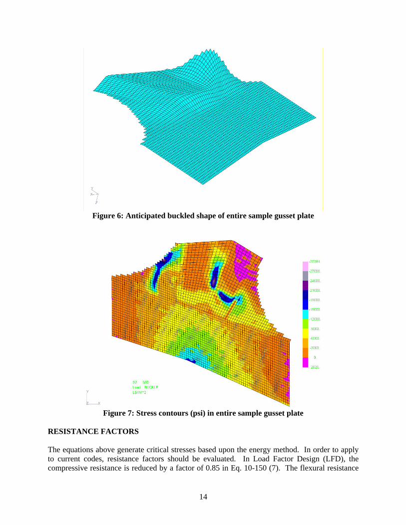
Figure 6: Anticipated buckled shape of entire sample gusset plate
Figure 7: Stress contours (psi) in entire sample gusset plate
RESISTANCE FACTORS The equations above generate critical stresses based upon the energy method. In order to apply to current codes, resistance factors should be evaluated. In Load Factor Design (LFD), the compressive resistance is reduced by a factor of 0.85 in Eq. 10-150 (7). The flexural resistance
14

of a column is not reduced, or has a factor of 1.0. In Load and Resistance Factor Design (LRFD), Section 6.5.4.2 of the code (8) gives the axial compressive resistance factor as 0.9 and the flexural resistance as 1.0. Resistance factors can readily be inserted into Eq. 24.
( zcccrit += )φσσ *1* Eq. 28 where φc is the compressive resistance factor, dependent upon the code used. As the bending resistance is 1.0 for both LFR and LRFR, there is no need to modify Eq. 28 for flexural resistance or Eq. 25 for the pure bending case. Should the critical buckling stress exceed the yield stress of the material, the yield stress would control. SUMMARY A solution to solving the combined axial and flexural stress resistance is needed in order to accurately load rate existing gusset plates. An approximate solution can be found using the Energy Method. This solution is conservative as it is developed based on a rectangular plate, while the actual shape is more likely triangular or trapezoidal. The increasing stiffness of the triangular shape will retard buckling at the extreme edge, and therefore the actual critical stress should be higher than that generated under this method. While this method is conservative, it is our belief that it more correctly models the plate resistance than the two methods currently proposed, either using the equation for buckling under pure compression or the yield strength of the material. The critical buckling stress for a gusset plate can be calculated as follows:
1. Calculate the concurrent forces in the plate. 2. Chose the sections to be analyzed, placing the sections so that the eccentricity is
maximized. 3. Calculate the axial stress, σc, based on the overall section dimensions and concurrent
forces. Load factors should be included. 4. Calculate the bending stress, σb, and yNA based on the overall section dimensions and
concurrent forces. Load factors should be included. 5. Set a equal to the unbraced length of the free edge. 6. Set b equal to the distance from the free edge to center of the joint. 7. Calculate z: 8. If 0=cσ then 0=z
c
bzσσ
= otherwise
9. Calculate σcrit:
15

If 0=cσ then ( )[ ]
y
NA
NA
crit f
yb
yb
batba
D
≤
⎟⎟⎠
⎞⎜⎜⎝
⎛−
+
+−=
3
1
*4
*6*1****3
22222 πυ
σ
( )[ ]yc
NA
NA
crit fz
ybz
ybz
batba
D
≤+
⎥⎥⎥⎥⎥
⎦
⎤
⎢⎢⎢⎢⎢
⎣
⎡⎟⎟⎠
⎞⎜⎜⎝
⎛−+
+
+−= )(*
3
1*1
*4*
*6*1****3
22222
φπυ
σ otherwise
10. Evaluate bccrit σσσ +≥ .
16

REFERENCES
1. Holt, R. and Hartmann, J (2008). Adequacy of the U10 & L11 Gusset Plate Designs for the Minnesota Bridge No. 9340 (I-35W over the Mississippi River) Interim Report. Federal Highway Administration. Turner-Fairbank Highway Research Center Report.
2. Ibrahim, F (2008). FHWA Bridge Design Guidance No 1: Load Rating Evaluation of
Gusset Plates in Truss Bridges. Federal Highway Administration.
3. Barson, J (1991). “Properties of Bridge Steels”. Highway Structures Design Handbook. Vol. I, Chap. 3. AISC. Pittsburgh, PA.
4. Lundquist, E., and Stowell, E. (1941). Critical Compressive Stress for Outstanding
Flanges. Report No. 734. Langley Memorial Aeronautical Laboratory, National Advisory Committee for Aeronautics. Langley Field, VA.
5. Timoshenko, S., and Gere, J. Theory of Elastic Stability. 2nd Ed. Singapore: Mc-Graw-
Hill Book Company, 1963. 6. Johnston, B. Guide to Stability Design Criteria for Metal Structures. 3rd Ed. New York:
John-Wiley &Sons, 1976.
7. AASHTO (2002). Standard Specifications for Highway Bridge Design, 17th Edition. Washington, DC.
8. AASHTO (2007). LRFD Bridge Design Specifications, 4th Edition. Washington, DC.
17

APPENDICES
18

Appendix A Comparison with Tabulated Values of Long Plates
Inputt .5in:= t 0.50 in=
ν .3:=
E 29 106psi×:=
DE t3×
12 1 ν2
−( )×:= D 331.96 kip in×=
Geometric and Stress Ratios
σc
1
1
0
⎛⎜⎜⎜⎝
⎞⎟⎟⎟⎠
ksi:=
σb
0
1
1
⎛⎜⎜⎜⎝
⎞⎟⎟⎟⎠
ksi:=
ratio 200:=
b 12in:=
a ratio b×:= a 2400.00 in=
yNAb2
:=
i 0 2..:=
Calculations
σ free σc σb+:= σ free
1.00
2.00
1.00
⎛⎜⎜⎜⎝
⎞⎟⎟⎟⎠
ksi=
σsimple σc σb+ σbb
yNA×−:= σsimple
1.00
0.00
1.00−
⎛⎜⎜⎜⎝
⎞⎟⎟⎟⎠
ksi=
zi 0 σci0=if
σbi
σci
otherwise
:= z
0.00
1.00
0.00
⎛⎜⎜⎜⎝
⎞⎟⎟⎟⎠
=
Appendix A Comparison with Tabulated Values of Long Plates
σcr_c_or_bi
D
3 a2× b2
× t×
π2 b2× 6 a2
× 1 ν−( )×+
b4 yNA×
1b
yNA−
3+
× σci0=if
D
3 a2× b2
× t×
π2 b2× 6 a2
× 1 ν−( )×+
zi b×
4 yNA×
1 zi 1b
yNA−
⎛⎜⎝
⎞⎟⎠
×+
3+
× otherwise
:= σcr_c_or_b
19.37
12.91
38.73
⎛⎜⎜⎜⎝
⎞⎟⎟⎟⎠
ksi=
σcr_linear_vary_loadiσcr_c_or_bi
σci0=if
σcr_c_or_bizi σcr_c_or_bi×+ otherwise
:=
σcr_linear_vary_load
19.37
25.82
38.73
⎛⎜⎜⎜⎝
⎞⎟⎟⎟⎠
ksi=
kequivσcr_linear_vary_load 12× 1 ν
2−( )× b2
×
π2 E× t2×
:= kequiv
0.43
0.57
0.85
⎛⎜⎜⎜⎝
⎞⎟⎟⎟⎠
=
Summary
Summary
"free edge stress"
σ free
ksi
"simple edge stress"
σsimple
ksi
"k.equiv"
kequiv
⎛⎜⎜⎜⎝
⎞⎟⎟⎟⎠
:=
Summary
"free edge stress"
1
2
1
⎛⎜⎜⎜⎝
⎞⎟⎟⎟⎠
"simple edge stress"
1
0
1−
⎛⎜⎜⎜⎝
⎞⎟⎟⎟⎠
"k.equiv"
0.426
0.567
0.851
⎛⎜⎜⎜⎝
⎞⎟⎟⎟⎠
⎡⎢⎢⎢⎢⎣
⎤⎥⎥⎥⎥⎦
=
Appendix B Comparison with Finite Element Analysisfor Various Geometries and Loadings
Inputt .5in:=
ν .3:=
E 29 106psi×:=
DE t3×
12 1 ν2
−( )×:= D 331.96 kip in×=
Geometric and Stress Ratios
σc
2
2
2
2
2
2
⎛⎜⎜⎜⎜⎜⎜⎜⎝
⎞⎟⎟⎟⎟⎟⎟⎟⎠
ksi:= σb
0
0
0
2
2
2
⎛⎜⎜⎜⎜⎜⎜⎜⎝
⎞⎟⎟⎟⎟⎟⎟⎟⎠
ksi:= b
18
36
18
18
36
18
⎛⎜⎜⎜⎜⎜⎜⎜⎝
⎞⎟⎟⎟⎟⎟⎟⎟⎠
in:= a
18
18
36
18
18
36
⎛⎜⎜⎜⎜⎜⎜⎜⎝
⎞⎟⎟⎟⎟⎟⎟⎟⎠
in:=
i 0 5..:=
yNAi
bi
2:=
Calculations
σ freeiσci
σbi+:= σ free
2.00
2.00
2.00
4.00
4.00
4.00
⎛⎜⎜⎜⎜⎜⎜⎜⎝
⎞⎟⎟⎟⎟⎟⎟⎟⎠
ksi= σsimpleiσci
σbi+ σbi
bi
yNAi
×−:= σsimple
2.00
2.00
2.00
0.00
0.00
0.00
⎛⎜⎜⎜⎜⎜⎜⎜⎝
⎞⎟⎟⎟⎟⎟⎟⎟⎠
ksi=
zi 0 σci0=if
σbi
σci
otherwise
:= z
0.00
0.00
0.00
1.00
1.00
1.00
⎛⎜⎜⎜⎜⎜⎜⎜⎝
⎞⎟⎟⎟⎟⎟⎟⎟⎠
=

Appendix B Comparison with Finite Element Analysisfor Various Geometries and Loadings
σcr_c_or_bi
D
3 ai( )2× bi( )2× t×
π2 bi( )2× 6 ai( )2× 1 ν−( )×+
bi
4 yNAi×
1bi
yNAi
−
3+
× σci0=if
D
3 ai( )2× bi( )2× t×
π2 bi( )2× 6 ai( )2× 1 ν−( )×+
zi bi×
4 yNAi×
1 zi 1bi
yNAi
−⎛⎜⎜⎝
⎞⎟⎟⎠
×+
3+
× otherwise
:=
σcr_c_or_b
28.83
22.38
13.66
19.22
14.92
9.11
⎛⎜⎜⎜⎜⎜⎜⎜⎝
⎞⎟⎟⎟⎟⎟⎟⎟⎠
ksi=
σcr_linear_vary_loadiσcr_c_or_bi
σci0=if
σcr_c_or_bizi σcr_c_or_bi×+ otherwise
:=σcr_linear_vary_load
28.83
22.38
13.66
38.44
29.83
18.22
⎛⎜⎜⎜⎜⎜⎜⎜⎝
⎞⎟⎟⎟⎟⎟⎟⎟⎠
ksi=
kequivi
σcr_linear_vary_loadi12× 1 ν
2−( )× bi( )2×
π2 E× t2×
:= kequiv
1.43
4.43
0.68
1.90
5.90
0.90
⎛⎜⎜⎜⎜⎜⎜⎜⎝
⎞⎟⎟⎟⎟⎟⎟⎟⎠
=
Summary
Summary
"a"
ain
"b"
bin
"simple edge stress"
σsimple
ksi
"free edge stress"
σ free
ksi
"k.equiv"
kequiv
⎛⎜⎜⎜⎝
⎞⎟⎟⎟⎠
:=
Summary
"a"
18
18
36
18
18
36
⎛⎜⎜⎜⎜⎜⎜⎜⎝
⎞⎟⎟⎟⎟⎟⎟⎟⎠
"b"
18
36
18
18
36
18
⎛⎜⎜⎜⎜⎜⎜⎜⎝
⎞⎟⎟⎟⎟⎟⎟⎟⎠
"simple edge stress"
2
2
2
0
0
0
⎛⎜⎜⎜⎜⎜⎜⎜⎝
⎞⎟⎟⎟⎟⎟⎟⎟⎠
"free edge stress"
2
2
2
4
4
4
⎛⎜⎜⎜⎜⎜⎜⎜⎝
⎞⎟⎟⎟⎟⎟⎟⎟⎠
"k.equiv"
1.426
4.426
0.676
1.901
5.901
0.901
⎛⎜⎜⎜⎜⎜⎜⎜⎝
⎞⎟⎟⎟⎟⎟⎟⎟⎠
⎡⎢⎢⎢⎢⎢⎢⎢⎢⎢⎣
⎤⎥⎥⎥⎥⎥⎥⎥⎥⎥⎦
=

Appendix C Comparison with Finite Element Analysis of
Sample Plate
Inputt .5in:=
ν .3:=
E 29 106psi×:=
DE t3×
12 1 ν2
−( )×:= D 331.96 kip in×=
Geometric and Stress Ratios
σc2
11.8⎛⎜⎝
⎞⎟⎠ksi:= σb
1.5
15.3⎛⎜⎝
⎞⎟⎠ksi:= b
45
34.5⎛⎜⎝
⎞⎟⎠in:= a
36.7
13.0⎛⎜⎝
⎞⎟⎠in:=
i 0 1..:=
yNAibi:=
Calculations
σ freeiσci
σbi+:= σ free
3.50
27.10⎛⎜⎝
⎞⎟⎠
ksi= σsimpleiσci
σbi+ σbi
bi
yNAi
×−:= σsimple2.00
11.80⎛⎜⎝
⎞⎟⎠
ksi=
zi 0 σci0=if
σbi
σci
otherwise
:= z0.75
1.30⎛⎜⎝
⎞⎟⎠
=
σcr_c_or_bi
D
3 ai( )2× bi( )2× t×
π2 bi( )2× 6 ai( )2× 1 ν−( )×+
bi
4 yNAi×
1bi
yNAi
−
3+
× σci0=if
D
3 ai( )2× bi( )2× t×
π2 bi( )2× 6 ai( )2× 1 ν−( )×+
zi bi×
4 yNAi×
1 zi 1bi
yNAi
−⎛⎜⎜⎝
⎞⎟⎟⎠
×+
3+
× otherwise
:=
σcr_c_or_b3.99
20.84⎛⎜⎝
⎞⎟⎠
ksi=

Appendix C Comparison with Finite Element Analysis of
Sample Plate
σcr_linear_vary_loadiσcr_c_or_bi
σci0=if
σcr_c_or_bizi σcr_c_or_bi×+ otherwise
:=σcr_linear_vary_load
6.99
47.87⎛⎜⎝
⎞⎟⎠
ksi=
kequivi
σcr_linear_vary_loadi12× 1 ν
2−( )× bi( )2×
π2 E× t2×
:= kequiv2.16
8.70⎛⎜⎝
⎞⎟⎠
=
Summary
Summary
"a"
ain
"b"
bin
"simple edge stress"
σsimple
ksi
"free edge stress"
σ free
ksi
"k.equiv"
kequiv
⎛⎜⎜⎜⎝
⎞⎟⎟⎟⎠
:=
Summary
"a"
36.7
13⎛⎜⎝
⎞⎟⎠
"b"
45
34.5⎛⎜⎝
⎞⎟⎠
"simple edge stress"
2
11.8⎛⎜⎝
⎞⎟⎠
"free edge stress"
3.5
27.1⎛⎜⎝
⎞⎟⎠
"k.equiv"
2.16
8.696⎛⎜⎝
⎞⎟⎠
⎡⎢⎢⎢⎣
⎤⎥⎥⎥⎦
=