1

23

Economist Sociologist Project Officer

Evaluating Anti-Poverty Programs:

Concepts and Methods

Martin RavallionDevelopment Research Group, World Bank

1. Introduction2. The evaluation problem3. Generic issues 4. Single difference: randomization5. Single difference: controls for observables6. Single difference: exploiting program design7. Double difference8. Higher-order differencing9. Instrumental variables10. Learning more from evaluations

• Assigned programs• some units (individuals, households, villages) get the program; • some do not.

• Examples:• Social fund selects from applicants• Workfare: gains to workers and benefiting communities; others get nothing• Cash transfers to eligible households only

• Ex-post evaluation• But ex post does not mean start late!

1. Introduction

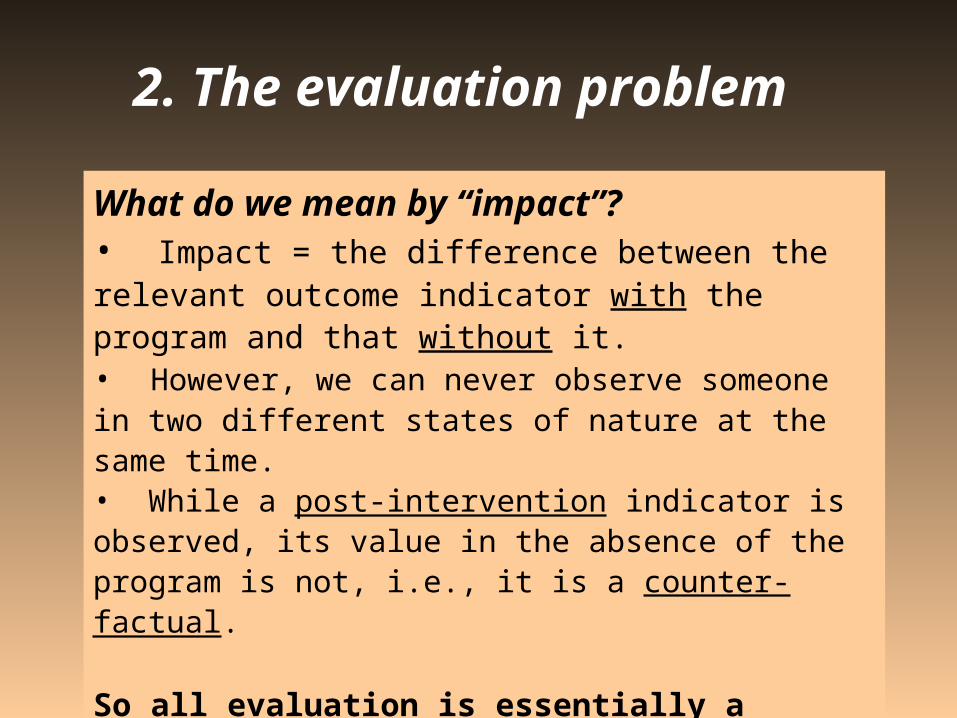
What do we mean by “impact”? • Impact = the difference between the relevant outcome indicator with the program and that without it.• However, we can never observe someone in two different states of nature at the same time. • While a post-intervention indicator is observed, its value in the absence of the program is not, i.e., it is a counter-factual.

So all evaluation is essentially a problem of missing data. Calls for counterfactual analysis.

2. The evaluation problem

Naïve comparisons can be deceptive

Common practices: compare outcomes after the intervention to those

before, or compare units (people, households, villages) that

receive the program with those that do not.

Potential biases from failure to control for: Other changes over time under the counterfactual, or Unit characteristics that influence program

placement.

Naïve comparison 1: Before vs after.We observe an outcome indicator,

Intervention

Y0

t=0 time

and its value rises after the program:

Y1 (observedl)

Y0

t=0 t=1 time

Intervention

However, we need to identify the counterfactual…

Y1 (observedl)

Y1

* (counterfactual)

Y0

t=0 t=1 time

Intervention

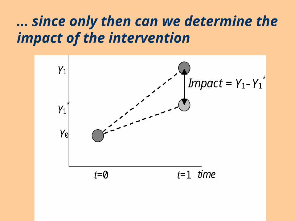
… since only then can we determine the impact of the intervention

Y1

Impact = Y1- Y1*

Y1

*

Y0

t=0 t=1 time

Naïve comparison 2: “With” vs.”without”

Impacts on poverty?

Percent not poor

Without(n=56)

43

43

With (n=44)

80

66

% increase(t-test)

87% (2.29)

54% (2.00)

Case 1

Case 2

Impacts on poverty?

Percent not poor

Without(n=56)

43

43

With (n=44)

80

66

% increase(t-test)

87% (2.29)

54% (2.00)

Case 1

Case 2

Without(n=56)

43

43

With (n=44)

80

66

% increase(t-test)

87% (2.29)

54% (2.00)

1: Program yields 20% gain

2: Program yields no gain

How can we do better? The missing-data problem in

evaluation For each unit (person, household, village,…)

there are two possible values of the outcome variable: The value under the treatment The value under the counterfactual

However, we cannot observe both for all units We cannot observe the counterfactual outcomes for

the treated units Or the outcomes under treatment for the untreated

units So evaluation is essentially a problem of missing

data => “counterfactual analysis.”

Outcomes (Y) with and without treatment (D) given exogenous covariates (X):

Ti

Ti

Ti XY (i=1,..,n)

Ci

Ci

Ci XY (i=1,..,n)

0)()( 10 iiii XEXE

Archetypal formulation

Outcomes (Y) with and without treatment (D) given exogenous covariates (X):

Ti

Ti

Ti XY (i=1,..,n)

Ci

Ci

Ci XY (i=1,..,n)

0)()( 10 iiii XEXE

Gain from the program: Ci

Tii YYG

ATE: average treatment effect: )( iGE

conditional ATE: )()( CTiii XXGE

ATET: ATE on the treated: )1( ii DGE

conditional ATET:

)1,()()1,( iiCi

Ti

CTiiii DXEXDXGE

Archetypal formulation

Given that we cannot observe CiY for 1iD or T

iY for 0iD , suppose we estimate the following model?

Ti

Ti

Ti XY if 1iD

Ci

Ci

Ci XY if 0iD

Or the (equivalent) switching regression:

iiCT

iC

iC

iiT

iii DXXYDYDY )()1( Ci

Ci

Tiii D )(

Common effects specification (only intercepts differ):

iC

iiCT

i XDY )( 00

The problem: X can be assumed exogenous but, without random assignment, D is endogenous => ordinary regression will give a biased estimate of impact.

The evaluation problem

Alternative solutions 1

Experimental evaluation (“Social experiment”) Program is randomly assigned, so that everyone

has the same probability of receiving the treatment.

In theory, this method is assumption free, but in practice many assumptions are required.

Pure randomization is rare for anti-poverty programs in practice, since randomization precludes purposive targeting.

Although it is sometimes feasible to partially randomize.

Alternative solutions 2

Non-experimental evaluation (“Quasi-experimental”; “observational studies”)One of two (non-nested) conditional independence assumptions:

1. Placement is independent of outcomes given X =>Single difference methods assuming conditionally exogenous program placement.

Or placement is independent of outcome changes =>Double difference methods

2. A correlate of placement is independent of outcomes given D and X

=> Instrumental variables estimator.

3. Generic issues

• Selection bias • Spillover effects

Selection bias in the outcome difference between

participants and non-participants

Observed difference in mean outcomes between participants (D=1) and non-participants (D=0):

)0()1( DYEDYE CT

)1()1( DYEDYE CT

ATET=average treatment effect on the treated

)0()1( DYEDYE CC

Selection bias=difference in mean outcomes (in the absence of the intervention) between participants and non-participants

= 0 with exogenousprogram placement

Two sources of selection bias

• Selection on observablesDataLinearity in controls?

• Selection on unobservablesParticipants have latent attributes that yieldhigher/lower outcomes

• One cannot judge if exogeneity is plausible without knowing whether one has dealt adequately with observable heterogeneity.• That depends on program, setting and data.

Spillover effects

• Hidden impacts for non-participants?

• Spillover effects can stem from:• Markets • Non-market behavior of participants/non-participants• Behavior of intervening agents (governmental/NGO)

• Example: Employment Guarantee Scheme • assigned program, but no valid comparison group.

• As long as the assignment is genuinely random, mean impact is revealed:

• ATE is consistently estimated (nonparametrically) by the difference between sample mean outcomes of participants and non-participants.

• Pure randomization is the theoretical ideal for ATE, and the benchmark for non-experimental methods.

• More common: randomization conditional on ‘X’

4. Randomization“Randomized out” group reveals counterfactual

)0()1( DYEDYE CC

Examples for developing countries

PROGRESA in Mexico Conditional cash transfer scheme 1/3 of the original 500 communities selected were

retained as control; public access to data Impacts on health, schooling, consumption

Proempleo in Argentina Wage subsidy + training Wage subsidy: Impacts on employment, but not

incomes Training: no impacts though selective compliance

Lessons from practice 1

Ethical objections and political sensitivities• Deliberately denying a program to those who need it and

providing the program to some who do not.• Yes, too few resources to go around. But is randomization the

fairest solution to limited resources?• What does one condition on in conditional randomizations?

• Intention-to-treat helps alleviate these concerns=> randomize assignment, but free to not participate

• But even then, the “randomized out” group may include people in great need.

=> Implications for design• Choice of conditioning variables.• Sub-optimal timing of randomization• Selective attrition + higher costs

Lessons from practice 2

Internal validity: Selective compliance

• Some of those assigned the program choose not to participate.

• Impacts may only appear if one corrects for selective take-up.

• Randomized assignment as IV for participation• Proempleo example: impacts of training only

appear if one corrects for selective take-up

Lessons from practice 3

External validity: inference for scaling up

• Systematic differences between characteristics of people normally attracted to a program and those randomly assigned (“randomization bias”: Heckman-Smith)

• One ends up evaluating a different program to the one actually implemented

=> Difficult in extrapolating results from a pilot experiment to the whole population

5.1 OLS regression

Ordinary least squares (OLS) estimator of impact with controls for selection on observables.

5. Controls Regression controls and matching

Switching regression:

iiCT

iC

iC

iiT

iii DXXYDYDY )()1( Ci

Ci

Tiii D )(

Common effects specification:

iC

iiCT

i XDY )( 00

OLS only gives consistent estimates under conditionally exogenous program placement

there is no selection bias in placement, conditional on X or (equivalently) that the conditional mean outcomes do not depend on treatment:

]0,[]1,[ ii

Ciii

Ci DXYEDXYE

Implying:

0],[ iii DXE in common impact model.

Even with controls…

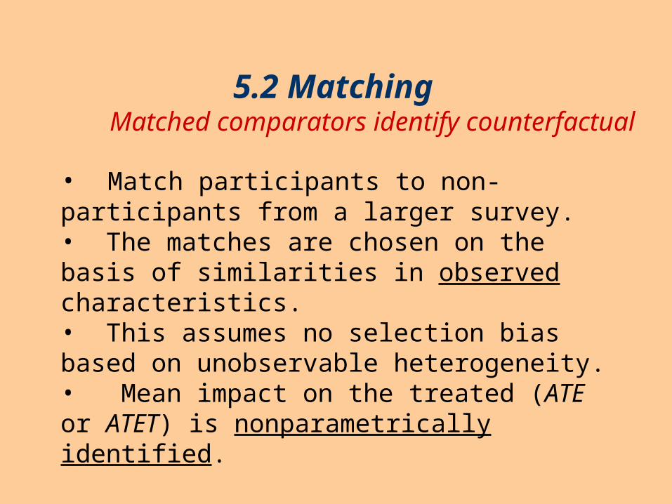
• Match participants to non-participants from a larger survey. • The matches are chosen on the basis of similarities in observed characteristics. • This assumes no selection bias based on unobservable heterogeneity.• Mean impact on the treated (ATE or ATET) is nonparametrically identified.

5.2 Matching Matched comparators identify counterfactual

Ideally we would match on the entire vector X of observed characteristics. However, this is practically impossible. X could be huge.

PSM: match on the basis of the propensity score (Rosenbaum and Rubin) =

This assumes that participation is independent of outcomes given X. If no bias given X then no bias given P(X).

Propensity-score matching (PSM) Match on the probability of

participation.

)1Pr()( iii XDXP

1: Representative, highly comparable, surveys of the non-participants and participants.

2: Pool the two samples and estimate a logit (or probit) model of program participation. Predicted values are the “propensity scores”.

3: Restrict samples to assure common support

Failure of common support is an important source of bias in observational studies (Heckman et al.)

Steps in score matching:

Density

0 1 Propensity score

Density of scores for participants

Density

0 1 Propensity score

Density of scores for non-participants

Density

0 Region of common support 1 Propensity score

Density of scores for non-participants

5: For each participant find a sample of non-participants that have similar propensity scores.

6: Compare the outcome indicators. The difference is the estimate of the gain due to the program for that observation.

7: Calculate the mean of these individual gains to obtain the average overall gain. Various weighting schemes =>

Steps in PSM cont.,

The mean impact estimator

NP

iijij

P

jj PYW - Y G

10

11 /)(

Various weighting schemes: Nearest k neighbors Kernel-weights (Heckman et al.,):

KK WP

jijijij

1

/

)]()([ jiij XPXPKK

Propensity-score weighting

PSM removes bias under the conditional exogeneity assumption.

However, it is not the most efficient estimator. Hirano, Imbens and Ridder show that weighting

the control observations according to their propensity score yields a fully efficient estimator.

Regression implementation for the common impact model:

with weights of unity for the treated units and for the controls.

iii DY

))(ˆ1/()(ˆ XPXP

How does PSM compare to an experiment?

PSM is the observational analogue of an experiment in which placement is independent of outcomes

The difference is that a pure experiment does not require the untestable assumption of independence conditional on observables.

Thus PSM requires good data. Example of Argentina’s Trabajar program

Plausible estimates using SD matching on good data

Implausible estimates using weaker data

How does PSM differ from OLS?

PSM is a non-parametric method (fully non-parametric in outcome space; optionally non-parametric in assignment space)

Restricting the analysis to common support

=> PSM weights the data very differently to standard OLS regression

In practice, the results can look very different!

How does PSM perform relative to other methods?

In comparisons with results of a randomized experiment on a US training program, PSM gave a good approximation (Heckman et al.; Dehejia and Wahba)

Better than the non-experimental regression-based methods studied by Lalonde for the same program.

However, robustness has been questioned (Smith and Todd)

Lessons on matching methods

When neither randomization nor a baseline survey are feasible, careful matching is crucial to control for observable heterogeneity.

Validity of matching methods depends heavily on data quality. Highly comparable surveys; similar economic environment

Common support can be a problem (esp., if treatment units are lost).

Look for heterogeneity in impact; average impact may hide important differences in the characteristics of those who gain or lose from the intervention.

Discontinuity designs• Participate if score M < m • Impact=

• Key identifying assumption: no discontinuity in counterfactual outcomes at m.• Strict eligibility rules alone do not make this plausible (e.g., geography and local govt.)• “Fuzzy” discontinuities in prob. participation.

6. Exploiting program design 1

)()( mMYEmMYE iC

iiT

i

Pipeline comparisons• Applicants who have not yet received program form the comparison group• Assumes exogeneous assignment amongst applicants• Reflects latent selection into the program

Exploiting program design 2

Lessons from practice

Know your program well: Program design features can be very useful for identifying impact.

Know your setting well too: Is it plausible that outcomes are continuous under the counterfactual?

But what if you end up changing the program to identify impact? You have evaluated something else!

Observed changes over time for non-participants provide the counterfactual for participants.

Steps:1. Collect baseline data on non-participants and

(probable) participants before the program. 2. Compare with data after the program. 3. Subtract the two differences, or use a regression

with a dummy variable for participant.

This allows for selection bias but it must be time-invariant and additive.

7. Difference-in-difference

Outcome indicator: t=0,1

where

= impact (“gain”);

= counterfactual;

= estimate from comparison group

itC

itT

it GYY

itG

CitY

CitY

Difference-in-difference

)]ˆ()ˆ[( 0011C

iT

iC

iT

i YYYYEDD

Baseline difference in outcomes

Post-intervention difference in outcomes

)]ˆˆ()[( 0101C

iC

iT

iT

i YYYYEDD

Gain over time for treatment group

Gain over time for comparison group

Or

Diff-in-diff: if (i) change over time for comparison group reveals counterfactual:

and (ii) baseline is uncontaminated by the program:

itC

iT

iC

iT

i GYYYYE )]ˆ()ˆ[( 0011

00 iG

Cit

Cit YEYE ˆ

Selection bias

Y1

Impact Y1

*

Y0

t=0 t=1 time

Selection bias

Diff-in-diff requires that the bias is additive and time-invariant

Y1

Impact Y1

*

Y0

t=0 t=1 time

The method fails if the comparison group is on a different trajectory Y1

Impact? Y1

*

Y0

t=0 t=1 time

=> DD overestimates impact

Or…

Y1

Y1

*

Y0

t=0 t=1 time

DD underestimates impactCommon problem in assessing impacts of development projects?

Example of poor area programs: areas not targeted yield a biased counter-factual

Not targeted

Targeted

Time

Income

• The growth process in non-treatment areas is not indicative of what would have happened in the targeted areas without the program• Example from China (Jalan and Ravallion)

Matched double differenceMatching helps control for time-varying

selection bias

• Score match participants and non-participants based on observed characteristics in baseline

• Initial conditions (incl. outcomes)

• Prior outcome trajectories

• Then do a double difference• This deals with observable heterogeneity in initial conditions that can influence subsequent changes over time

Propensity-score weighted version of “matched diff-in-diff.”

Weighting the control observations according to their propensity score yields a fully efficient estimator (Hirano, Imbens and Ridder).

Regression:

with weights of unity for the treated units and

for the controls where

is the propensity score.

)(11 DDDtDY ittiiit

))(ˆ1/()(ˆ XPXP )1Pr()( iii XDXP

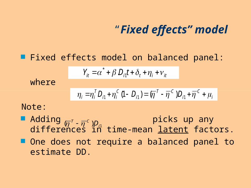
“Fixed effects” model

Fixed effects model on balanced panel:

where

Note: Adding picks up any differences in time-

mean latent factors. One does not require a balanced panel to estimate

DD.

iC

iCT

iCii

Tii DDD 111 )()1(

ititiit tDY 1* .

1)( iCT D

Lessons from practice

Single-difference matching can be severely contaminated by selection bias Latent heterogeneity in factors relevant to participation

Tracking individuals over time allows a double difference This eliminates all time-invariant additive selection bias

Combining double difference with matching: This allows us to eliminate observable heterogeneity in

factors relevant to subsequent changes over time

8. Higher-order differencing

Pre-intervention baseline data unavailable

e.g., safety net intervention in response to a crisis

Can impact be inferred by observing participants’ outcomes in the absence of the program after the program?

New issues

Selection bias from two sources:

1. decision to join the program

2. decision to stay or drop out There are observed and unobserved characteristics

that affect both participation and income in the absence of the program

Past participation can bring current gains for those who leave the program

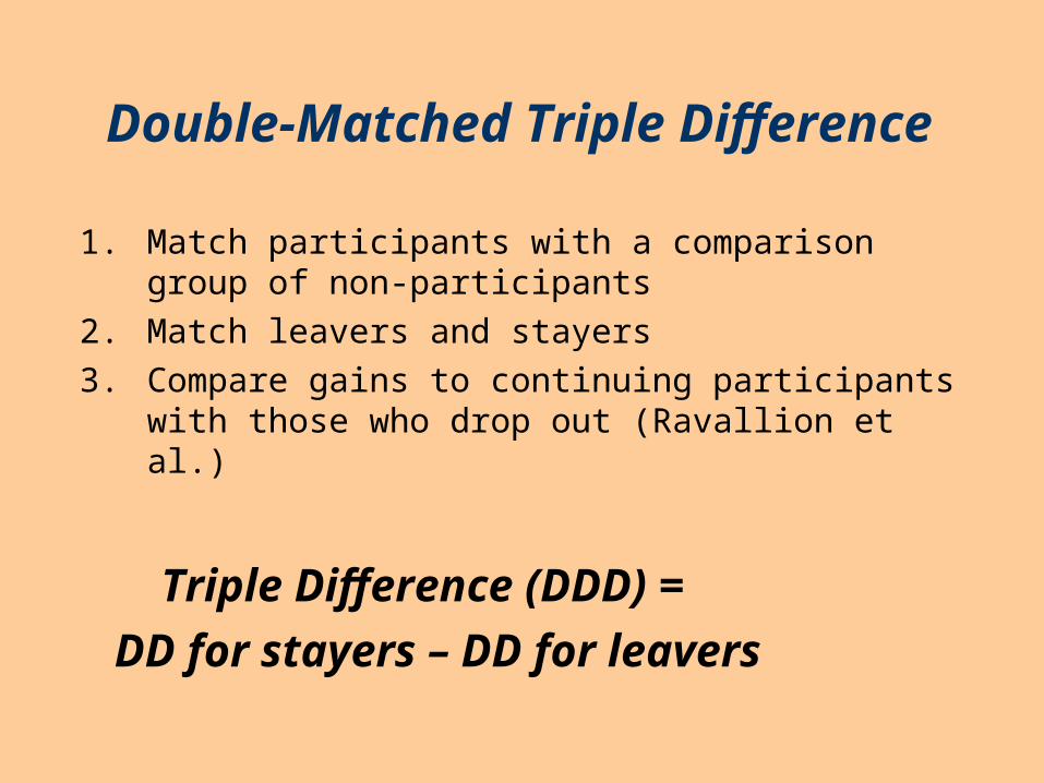
Double-Matched Triple Difference

1. Match participants with a comparison group of non-participants

2. Match leavers and stayers

3. Compare gains to continuing participants with those who drop out (Ravallion et al.)

Triple Difference (DDD) = DD for stayers – DD for leavers

Outcomes for participants:

Single difference:

Double difference:

Triple difference:

“stayers” “leavers” in period 2 in period 2

itC

itT

it GYY

][ Cit

Tit YYE

itC

itTit GYYE )]([

]0)([]1)([ 222222 iC

iT

iiC

iT

i DYYEDYYE

)]0()1([

)]0()1([

2121

2222

iiii

iiii

DGEDGE

DGEDGE net gain from participation

selection bias

]0)([]1)([ 222222 iC

iT

iiC

iT

i DYYEDYYE

Joint conditions for DDD to estimate impact:

no current gain to ex-participants;

no selection bias in who leaves the program;

)0( 22 ii DGE

)0()1( 2121 iiii DGEDGE

Sign of the selection bias? If leavers have lower gains then DDD underestimates impact

Test for whether DDD identifies gain to current

participants

Third round of data allows a test: mean gains in round 2 should be the same whether or not one drops out in round 3

)0,1()1,1( 322322 iiiiii DDGEDDGEDDD

Gain in round 2 forstayers in round 3

Gain in round 2 forleavers in round 3

Lessons from practice

1. Tracking individuals over time: addresses some of the limitations of single-difference

on weak data allows us to study the dynamics of recovery

2. “Baseline” can be after the program, but must address the extra sources of selection bias

3. Single difference for leavers vs. stayers can work well if there is an exogenous program contraction

9. Instrumental variables Identifying exogenous variation using a 3rd

variable

Outcome regression:

(D = 0,1 is our program – not random)

• “Instrument” (Z) influences participation, but does not affect outcomes given participation (the “exclusion restriction”).

• This identifies the exogenous variation in outcomes due to the program.

Treatment regression:

iii DY

iii uZD

Reduced-form outcome regression:

where and

Instrumental variables (two-stage least squares) estimator of impact:

Or:

iiiiii ZuZY )(

OLSOLSIVE ˆ/ˆˆ

iii u

iii ZY )ˆ(

Predicted D purged of endogenous part.

Problems with IVE

1. Finding valid IVs; Usually easy to find a variable that is correlated with

treatment. However, the validity of the exclusion restrictions

is often questionable.

2. Impact heterogeneity due to latent factors

Sources of instrumental variables

Partially randomized designs as a source of IVs Non-experimental sources of IVs

Geography of program placement (Attanasio and Vera-Hernandez); “Dams” example (Duflo and Pande)

Political characteristics (Besley and Case; Paxson and Schady)

Discontinuities in survey design

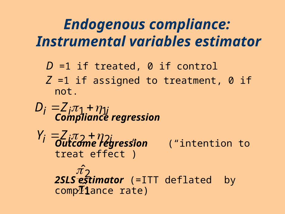
Endogenous compliance: Instrumental variables estimator

D =1 if treated, 0 if control

Z =1 if assigned to treatment, 0 if not.

Compliance regression

Outcome regression (“intention to treat effect”)

2SLS estimator (=ITT deflated by compliance rate)

iii ZD 11

iii ZY 22

1

2ˆˆ

Essential heterogeneity and IVE

Common-impact specification is not harmless. Heterogeneity in impact can arise from

differences between treated units and the counterfactual in latent factors relevant to outcomes.

For consistent estimation of ATE we must assume that selection into the program is unaffected by latent, idiosyncratic, factors determining the impact (Heckman et al).

However, likely “winners” will no doubt be attracted to a program, or be favored by the implementing agency.

=> IVE is biased even with “ideal” IVs.

IVE identifies the effect for those induced to switch by the instrument (“local average effect”) Suppose Z takes 2 values. Then the effect of the program is:

Care in extrapolating to the whole population when there is latent heterogeneity.

IVE is only a ‘local’ effect

)0|()1|(

)0|()1|(

ZDEZDE

ZYEZYEIVE

LIV directly addresses the latent heterogeneity problem. The method entails a nonparametric regression of outcomes Y on the propensity score.

The slope of the regression function gives the marginal impact at the data point.

This slope is the marginal treatment effect (Björklund and Moffitt), from which any of the standard impact parameters can be calculated (Heckman and Vytlacil).

Local instrumental variables

iiii XZPfY )](ˆ[)](ˆ[ iZPf

Lessons from practice Partially randomized designs offer great source of

IVs. The bar has risen in standards for non-

experimental IVE Past exclusion restrictions often questionable in

developing country settings However, defensible options remain in practice, often

motivated by theory and/or other data sources Future work is likely to emphasize latent

heterogeneity of impacts, esp., using LIV.

10. Learning from evaluations

Can the lessons be scaled up? What determines impact?

Is the evaluation answering the relevant policy questions?

Scaling up?

Institutional context => impact; “in certain settings anything works, in others everything fails”

Local contextual factors in development impact Example of Bangladesh’s Food-for-Education

program Same program works well in one village, but fails

hopelessly nearby Partial equilibrium assumptions are fine for a pilot

but not when scaled up PE greatly overestimates impact of tuition subsidy

once relative wages adjust (Heckman)

What determines impact? Replication across differing contexts

Example of Bangladesh’s FFE: inequality etc within village => outcomes of program

Implications for sample design => trade off between precision of overall impact estimates and ability to explain impact heterogeneity

Intermediate indicators Example of China’s SWPRP Small impact on consumption poverty But large share of gains were saved

Qualitative research/mixed methods Test the assumptions (“theory-based evaluation”) But poor substitute for assessing impacts on final

outcome

Policy-relevant questions? Choice of counterfactual Policy-relevant parameters?

Mean vs. poverty (marginal distribution) Average vs. marginal impact Joint distribution of YT and YC , esp., if some

participants are worse off: ATE only gives net gain for participants.

“Black box” vs. Structural parameters Simulate changes in program design PROGRESA example (Attanasio et al.; Todd&Wolpin)

• Modeling schooling choices using randomized assignment for identification

• Budget-neutral switch from primary to secondary subsidy would increase impact

Conclusion: What not to do!

You know a bad evaluation when you see it: Evaluation process is poorly linked to project

Evaluator did not know enough about setting and project Data collection started too late Data collection did not cover right outcomes and did not

allow for adequate controls• Too many “monitoring indicators” + too few outcomes and

controls Evaluation did not address, or even ask, the right questions!

No basis for assessing the counterfactual No comparison group; no historical data Too little data for addressing endogenous program

placement Not enough thought about selection bias and spillovers