Electronic Supplementary Material (ESI) for Soft Matter.This journal is © The Royal Society of Chemistry 2017

Supporting Information for:

Dissipative Particle Dynamics Simulation Study on Phase Diagrams for the Self-Assembly

of Amphiphilic Hyperbranched Multiarm Copolymers in Various Solvent Conditions

Haina Tan,a Chunyang Yu,*a Zhongyuan Lu*b, Yongfeng Zhou,*a and Deyue Yana

1. The detailed information about the coarse-grained DPD models.

The amphiphilic hyperbranched multiarm copolymers HBPO-star-PEO with one hydrophobic

hyperbranched HBPO core and many hydrophilic linear PEO arms (ref. 23) could be considered

as the representative prototype for the coarse-grained DPD model used in this paper. As listed in

Table S1, the volumes of the repeat units in the HBPO-star-PEO molecule can be calculated

according to the experimental density and molecular weight. Because all of the beads are

assumed to possess the same volume in DPD simulation, so we used one A bead (the yellow

bead) in the model to represent one repeat unit of HBPO, while one B bead (the cyan bead)

represents three repeat units of PEO. Moreover, when the solvent is water (V = 30 Å3), one S

bead represents six water molecules.

Table S1 Molecular parameters in the system of HBPO-star-PEO copolymers.

Bead typeMolecular weight

M (g/mol)

Density

ρ (g/cm3)

Monomer

volume V (Å3)

A (Hydrophobic HBPO) 116 1.0 193

B (Hydrophilic PEO) 44 1.12 65

2. The explanation for the interaction between water molecules by applying soft repulsion

potential.

According to the reports by Groot and Warren (ref. 61), the dimensionless compressibility can be

described by κ-1 ≈ 1 + 0.2αiiρ/kBT, where αii is repulsion parameter between the same type of

bead, ρ is number density, and the temperature kBT is taken as the reduced units. Considering

that κ-1 equals 15.9835 for water at room temperature (300K), the repulsion parameter αii is

calculated to be 25 when ρ equals 3. Therefore, it is correct to describe interaction between water

molecules by applying soft repulsion potential in DPD simulations.

1

Electronic Supplementary Material (ESI) for Soft Matter.This journal is © The Royal Society of Chemistry 2017

3. HOOMD scripts used for DPD simulations.

from hoomd_script import *

init.read_xml(filename="xxxxxx.xml") # xxxxxx.xml is the input file

#specify interaction parameters between particle pairs

dpd = pair.dpd(r_cut=1.0, T=1.0)

dpd.pair_coeff.set('A', 'A', A=25.00, gamma = 4.5)

dpd.pair_coeff.set('A', 'B', A=50.0, gamma = 4.5)

dpd.pair_coeff.set('A', 'S', A=as.0, gamma = 4.5) # as.0 is the value of αAS

dpd.pair_coeff.set('B', 'B', A=25.00, gamma = 4.5)

dpd.pair_coeff.set('B', 'S', A=bs.0, gamma = 4.5) # bs.0 is the value of αBS

dpd.pair_coeff.set('S', 'S', A=25.00, gamma = 4.5)

dpd.set_params(T = 1.0)

nlist.set_params(r_buff = 0.25)

nlist.reset_exclusions(exclusions = [])

harmonic = bond.harmonic()

harmonic.set_coeff('bond1', k=4.0, r0=0.0) # k=4.0 is the coefficient of harmonic spring force

# define the type

groupA = group.type(name='groupA', type='A')

groupB = group.type(name='groupB', type='B')

groupAB = group.union(name="groupAB", a=groupA, b=groupB)

groupC = group.type(name='groupC', type='S')

groupABC = group.union(name="groupABC", a=groupAB, b=groupC)

integrate.mode_standard(dt=0.02) # dt=0.02 is the integration time step

integrate.nve(group=group.all())

2

# output files

analyze.log(filename="dpdnve_energy.log", quantities=['potential_energy', 'kinetic_energy'],

period=100, header_prefix='#', overwrite=True)

analyze.log(filename='dpdmomentum.log', quantities=['momentum'], period=100,

header_prefix='#', overwrite=True)

analyze.log(filename='dpdtemperature.log', quantities=['temperature'], period=100,

header_prefix='#', overwrite=True)

xml = dump.xml(filename="particles", period=1000000)

xml.set_params(position=True, type=True, bond=True)

dump.bin(filename="particles", period=2000000)

mol2 = dump.mol2()

mol2.write(filename="zinitial.mol2")

dump.dcd(filename="ztrajectory.dcd", period=10000, group=groupAB)

# run 4000000 time steps

run(4000001)

3

Fig. S1 The morphological snapshots of the spherical micelles formed by A42B20 at αBS = 5 and

αAS = 50 (a), αBS = 23 and αAS = 50 (b); (c) the relationships between Nmicelle and αBS (blue curve),

mean aggregation number and αBS (green curve) at αAS = 50, respectively. Error bars are

obtained by averaging five parallel samples. The solvent beads are omitted for clarity. The color

codes are the same as those in Fig. 2.

4

Fig. S2 Sequential snapshots of the formation of the vesicle with a membrane inside self-

assembled from Fig. 4c at 1.50 × 105 steps (a), 1.90 × 105 steps (b), 2.20 × 105 steps (c), 2.80 ×

105 steps (d), 7.90 × 105 steps (e), to 1.65 × 106 steps (f). For each image, the upper one is the 3D

view, while the lower one is the cross-section view. The solvent beads are omitted for clarity.

The color codes are the same as those in Fig. 2.

5

Fig. S3 The fine structure of one vesicle: (a) cross-sectional view of the vesicle showing the

membrane structure, and the arrow indicates the two labelled molecules extracted from the

vesicle to show the molecular packing model. (b) Radial density distributions of A (yellow) and

B (cyan) segments across the membrane of the vesicle. The distance from the centre of mass to

the outside of the vesicle is r. Hydrophobic hyperbranched core: yellow, red, and purple beads;

hydrophilic linear arms: cyan, green, and blue beads.

6

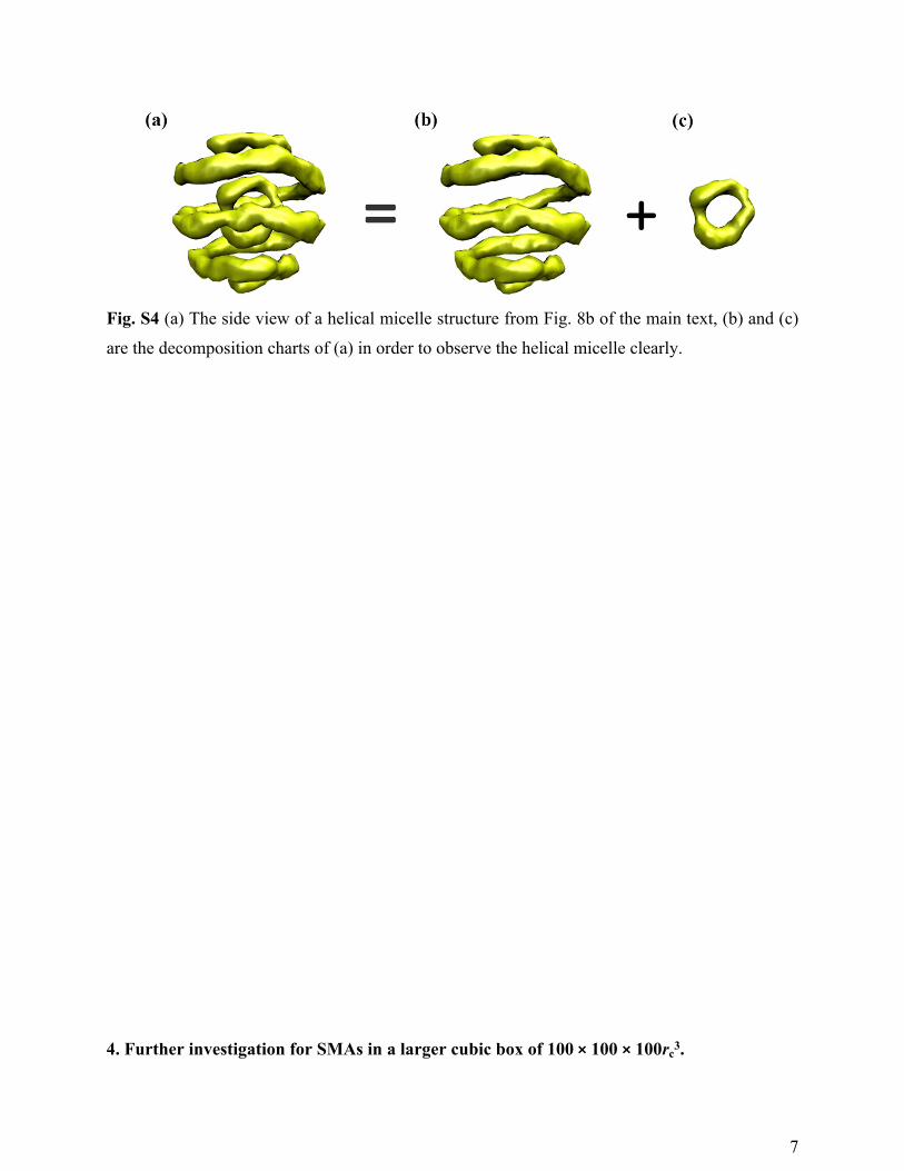
Fig. S4 (a) The side view of a helical micelle structure from Fig. 8b of the main text, (b) and (c)

are the decomposition charts of (a) in order to observe the helical micelle clearly.

4. Further investigation for SMAs in a larger cubic box of 100 × 100 × 100rc3.

7

Furthermore, we have carried out the simulation for the formation of small micelle aggregates

(SMAs) in a larger cubic box of 100 × 100 × 100rc3 (αBS = 29, αAS = 80). There are a total of

seven SMAs in the box at 4.00 × 106 time steps (Fig. S5). Among the seven SMAs, five of them

are separated into several aggregates on the wall of the box by the periodic boundary conditions

applied in all three dimensions. Then, we calculated the distribution of the aggregation number

(Nagg) versus the simulation time. As depicted in Fig. S6, with the increase of the simulation

time, Nagg first decreases and then levels off from 1.00 × 106 to 4.00 × 106 time steps. Such a

result indicated that the polymers began to self-assemble and then reached equilibrium in the

simulation box. Moreover, we also calculated the time evolution of conservative energy EAS (Fig.

S7). At the beginning, EAS decreases sharply and quickly, and then decreases slowly and finally

reaches a relative dynamic equilibrium state. The average shape factor of the seven SMAs is

0.425, and the variance of the average shape factor is 0.264, which attributes to the different

number of small spherical micelle in every SMAs.

Fig. S5 The final snapshot of SMAs at 4.00 × 106 time steps in a cubic box of 100 × 100 ×

100rc3. The left one is the 3D view, while the right one is the isosurface view of type A. The

solvent beads are omitted for clarity.

8

Fig. S6 The distribution of Nagg versus the simulation time for the SMAs.

Fig. S7 Conservative energy between the hyperbranched core beads and the solvents, EAS versus

simulation time.

9