0dvwhu 7khvlv 5hsruw - umu.diva-portal.org1260601/fulltext01.pdf · industrial supervisor - scania...
TRANSCRIPT

Master Thesis ReportRisk Assessment based Data Augmentation for Robust ImageClassification
using Convolutional Neural Network
Harisubramanyabalaji Subramani Palanisamy
November 4, 2018
StudentSpring 2018Master Thesis, 30 ECTSMaster of Science in Applied Physics and Electronics (Specialization in Robotics and Control), 120 ECTS
Risk Assessment based DataAugmentation for Robust Image
Classification
Harisubramanyabalaji Subramani Palanisamy
November 4, 2018Master’s Thesis in Robotics and Control
Academic Supervisor - Umea: Shafiq ur RehmanIndustrial Supervisor - Scania CV AB: Mattias Nyberg & Joakim Gustavsson
Examiner: John Berge
UmeaUniversityDepartment of Applied Physics and Electronics
SE-901 87 UMEASWEDEN


Abstract
Autonomous driving is increasingly popular among people and automotive industries inrealizing their presence both in passenger and goods transportation. Safer autonomousnavigation might be very challenging if there is a failure in sensing system. Among severalsensing systems, image classification plays a major role in understanding the road signs andto regulate the vehicle control based on urban road rules. Hence, a robust classifier algorithmirrespective of camera position, view angles, environmental condition, different vehicle size& type (Car, Bus, Truck, etc.,) of an autonomous platform is of prime importance.
In this study, Convolutional Neural Network (CNN) based classifier algorithm has beenimplemented to ensure improved robustness for recognizing traffic signs. As training dataplay a crucial role in supervised learning algorithms, there come an effective dataset re-quirement which can handle dynamic environmental conditions and other variations causeddue to the vehicle motion (will be referred as challenges). Since the collected training datamight not contain all the dynamic variations, the model weakness can be identified by ex-posing it to variations (Blur, Darkness, Shadow, etc.,) faced by the vehicles in real-time as ainitial testing sequence. To overcome the weakness caused due to the training data itself, aneffective augmentation technique enriching the training data in order to increase the modelcapacity for withstanding the variations prevalent in urban environment has been proposed.
As a major contribution, a framework has been developed to identify model weakness andsuccessively introduce a targeted augmentation methodology for classification improvement.Targeted augmentation is based on estimated weakness caused due to the challenges withdifficulty levels, only those necessary for better classification were then augmented further.Predictive Augmentation (PA) and Predictive Multiple Augmentation (PMA) are the twoproposed methods to adapt the model based on targeted challenges by delivering with highnumerical value of confidence. We validated our framework on two different training datasets(German Traffic Sign Recognition Benchmark (GTSRB) and Heavy Vehicle data collectedfrom bus) and with 5 generated test groups containing varying levels of challenge (simpleto extreme). The results show impressive improvement by ≈ 5-20% in overall classificationaccuracy thereby keeping their high confidence.
Keywords: Safety-Risk assessment, predictive augmentation, convolutional neural net-work, traffic sign classification, autonomous driving, heavy vehicles, orientation challenges,classification degradation.

ii

Acknowledgement
I am extremely privileged to thank everyone who helped me getting motivated and sup-ported me in successfully completing my master study.
First and Foremost, I would like to express my sincere gratitude to my academic advisorAssociate Prof. Shafiq ur Rehman and industrial advisor Prof. Mattias Nyberg & JoakimGustavsson for their continuous support in my thesis research, and their patience. I amthankful for the inspirations and encouragement in writing of this thesis.
It is my pleasure to thank my manager Marcus, EPXS department, Scania and my col-leagues Xinyi, Nazre, Noren, Mikael, Agneev, Sandipan, Yash, Dave, Maz, and Christianfor their support.
Besides my advisor, I would like to thank Sikandar Lal Khan, who helped me in strength-ening my skills focusing novel computer vision algorithms and providing me with moralsupport to follow my dream.
I am truly indebted and thankful to my fellow friends Sribalaji and Abhishek for con-stantly having several technical discussions in bringing novel solutions to existing problemand supporting me in hard times during my master study.
Many thanks to my family: parents (Palanisamy and Padmavathi), sister (PrabhaKarthikeyan) for supporting me, understanding my decisions and being there all along inthis wonderful journey. Without them I would have not reached this position.
Last but not the least, I would like to thank my friends who made my stay in Umea verywonderful; Shreyas, Aravind, Alieu, Ashokan, Rahul,Vishnupradeep, Mahmoud Sukkar, LiSongyu, Xiaowei, Adam, Ariane, Midhu, Mi, Vishnu, Sushmitha, Senthil, Kavya.
Thank you everyone .
Harisbramanyabalaji Subramani PalanisamyUmea University, Sweden, 2018
iii

iv

Preface
Part of the work presented in this thesis have passed peer-reviewed conference proceedings.
1. Harisubramanyabalaji Subramani Palanisamy, Shafiq ur Rehman, Mattias Nyberg,and Joakim Gustavsson, “Improving Image Classification Robustness UsingPredictive Data Augmentation”, 1st SAFECOMP Workshop on Artificial Intel-ligence Safety Engineering, WAISE 2018, September 18-21,Vasteras, Sweden.
v

vi

Contents
Abstract . . . . . . . . . . . . . . . . . . . . . . . . . . . . . . . . . . . . . . . . . . i
Acknowledgement . . . . . . . . . . . . . . . . . . . . . . . . . . . . . . . . . . . . iii
Preface . . . . . . . . . . . . . . . . . . . . . . . . . . . . . . . . . . . . . . . . . . v
1 Introduction 1
1.1 Motivation . . . . . . . . . . . . . . . . . . . . . . . . . . . . . . . . . . . . . 1
1.2 Contribution and Scope . . . . . . . . . . . . . . . . . . . . . . . . . . . . . . 5
1.3 Related Work . . . . . . . . . . . . . . . . . . . . . . . . . . . . . . . . . . . . 6
1.4 Thesis Overview . . . . . . . . . . . . . . . . . . . . . . . . . . . . . . . . . . 8
2 Background & Theory 9
2.1 Artificial Neural Networks (ANN) . . . . . . . . . . . . . . . . . . . . . . . . 9
2.1.1 Layers . . . . . . . . . . . . . . . . . . . . . . . . . . . . . . . . . . . . 10
2.2 Convolutional Neural Network (CNN) . . . . . . . . . . . . . . . . . . . . . . 12
2.2.1 Convolution Layer . . . . . . . . . . . . . . . . . . . . . . . . . . . . . 13
2.2.2 Pooling Layer . . . . . . . . . . . . . . . . . . . . . . . . . . . . . . . . 13
2.2.3 Fully Connected Layer . . . . . . . . . . . . . . . . . . . . . . . . . . . 14
2.2.4 Loss Function . . . . . . . . . . . . . . . . . . . . . . . . . . . . . . . . 14
2.2.5 Optimization . . . . . . . . . . . . . . . . . . . . . . . . . . . . . . . . 14
2.3 Image Manipulation . . . . . . . . . . . . . . . . . . . . . . . . . . . . . . . . 15
3 Assessment and Augmentation Method 21
3.1 Safety-Risk Assessment and Augmentation Framework . . . . . . . . . . . . . 21
3.1.1 Safe-Risk Assessment . . . . . . . . . . . . . . . . . . . . . . . . . . . 23
3.1.2 Predictive Augmentation . . . . . . . . . . . . . . . . . . . . . . . . . 23
4 Experiments 25
4.1 Dataset Selection . . . . . . . . . . . . . . . . . . . . . . . . . . . . . . . . . . 25
4.2 CNN Architecture Selection . . . . . . . . . . . . . . . . . . . . . . . . . . . . 26
4.3 Challenge Generation . . . . . . . . . . . . . . . . . . . . . . . . . . . . . . . 28
4.4 Experiment 1 : Robustness Verification . . . . . . . . . . . . . . . . . . . . . 31
4.4.1 Results . . . . . . . . . . . . . . . . . . . . . . . . . . . . . . . . . . . 33
vii

viii CONTENTS
4.5 Experiment 2: Model Capacity Identification . . . . . . . . . . . . . . . . . . 38
4.5.1 Results . . . . . . . . . . . . . . . . . . . . . . . . . . . . . . . . . . . 38
4.6 Experiment 3: Predictive Augmentation . . . . . . . . . . . . . . . . . . . . . 43
4.6.1 Results . . . . . . . . . . . . . . . . . . . . . . . . . . . . . . . . . . . 43
5 Discussion 49
6 Conclusions 51
References 53
A Experiment 1 Results 59

List of Figures
1.1 Experimental camera locations and respective field of view to cover the scene
around the vehicle. Based on vehicle size and type, location of cameras are
being altered and calibrated. . . . . . . . . . . . . . . . . . . . . . . . . . . . 2
1.2 Image captured from different location on heavy vehicle leads to orientation
change in captured objects taken from [26]. Left: Front View, Right: Top
View . . . . . . . . . . . . . . . . . . . . . . . . . . . . . . . . . . . . . . . . . 2
1.3 Prototype autonomous heavy vehicle with six camera location and their re-
spective images to show variation in orientation of a traffic signs. Figure in
column 1: Targeted left side environment (Top: forward left and Bottom:
rear left), column 2: Targeted middle environment (Top: forward front and
Bottom: rear front), column 3: Targeted right side environment (Top:
forward right and Bottom: rear right) . . . . . . . . . . . . . . . . . . . . . . 3
1.4 Natural environmental variations captured by the front facing camera placed
on heavy vehicle and classifier clearly misses the traffic sign of our interest . . 4
1.5 Natural variations exist in collected GTSRB dataset taken from [27] . . . . . 5
1.6 State-of-the-art CNN architectures for image classification . . . . . . . . . . 7
2.1 Simple perceptron representation with multi input and single output (solid
box as they represent constants). X1...Xn are inputs and W1...Wn are learn-
ing weights (hollow box as they represent variables) . . . . . . . . . . . . . . 9
2.2 Single hidden layer based Artificial Neural Network with 1-D feature vector
as input sample and four class output . . . . . . . . . . . . . . . . . . . . . . 10
2.3 Multiple hidden layer based Deep Neural Network (DNN) [58] . . . . . . . . . 10
2.4 Activation functions for neural networks [61] . . . . . . . . . . . . . . . . . . 12
2.5 Schema of weight flow in gradient descent algorithm, targeted to bring ini-
tialized weight to global minimum [64] . . . . . . . . . . . . . . . . . . . . . . 12
2.6 Rolling variation of image can be generated both in clockwise and anti-
clockwise direction with defined angles . . . . . . . . . . . . . . . . . . . . . . 16
2.7 Pitch variation of image can be generated in order compensate the Top and
Bottom view of an object . . . . . . . . . . . . . . . . . . . . . . . . . . . . . 17
ix

x LIST OF FIGURES
2.8 Yaw variation of image can be generated in order compensate the view from
Left and Right side of an object . . . . . . . . . . . . . . . . . . . . . . . . . . 17
2.9 Occlusion variation of image can be generated in order compensate the changes
occurring in any part of an object . . . . . . . . . . . . . . . . . . . . . . . . 18
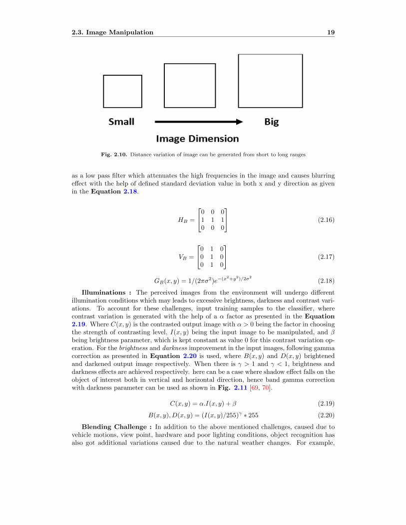
2.10 Distance variation of image can be generated from short to long ranges . . . . 19
2.11 Shadow variation can be generated both in horizontal and vertical direction
of an object . . . . . . . . . . . . . . . . . . . . . . . . . . . . . . . . . . . . . 20
2.12 Blending of two input images in order to create overlapping challenges on one
image . . . . . . . . . . . . . . . . . . . . . . . . . . . . . . . . . . . . . . . . 20
3.1 Schematic flow chart to represent the Safety-Risk assessment and augmen-
tation framework for traffic sign classification with training (TR), validation
(VR), and testing (TE) being the input data. Identified weakness in terms of
challenge type and its difficulty level (Risk Ranges) are used by the predictive
augmentation platform to improve the training and validation samples . . . . 22
3.2 Systematic selection of safe and risk ranges based on defined threshold recog-
nition accuracy for each challenge type . . . . . . . . . . . . . . . . . . . . . . 24
4.1 Sample images collected from dataset considered for this study with natu-
ral variations. Left: German Traffic Sign Recognition Benchmark Right:
Collected heavy vehicle data with four class types . . . . . . . . . . . . . . . . 26
4.2 CNN Architecture : Input→ CV1→ PL1→ CV2→ PL2→ FC1→ FC2→FC3 (Output). Convolution layer(CV), Polling Layer(PL), Fully connected
layer (FC), and feature reduction corresponding to each layer in terms of
image dimension is embedded inside blocks . . . . . . . . . . . . . . . . . . . 27
4.3 Systematic selection of hyper parameters, with Lr, Fd, D, B, Fk being
Learning rate, Filter depth, Nodes in hidden layers, Batch size, and Filter
kernel size respectively . . . . . . . . . . . . . . . . . . . . . . . . . . . . . . . 27
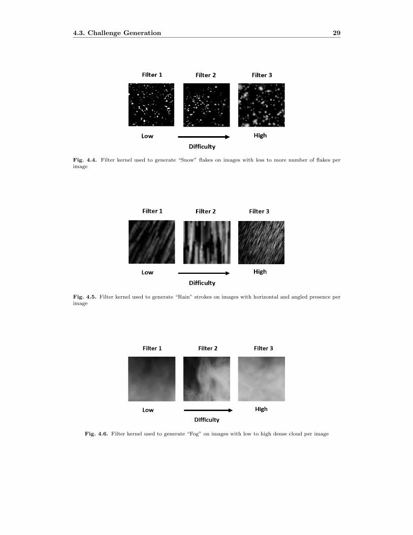
4.4 Filter kernel used to generate “Snow” flakes on images with less to more
number of flakes per image . . . . . . . . . . . . . . . . . . . . . . . . . . . . 29
4.5 Filter kernel used to generate “Rain” strokes on images with horizontal and
angled presence per image . . . . . . . . . . . . . . . . . . . . . . . . . . . . . 29
4.6 Filter kernel used to generate “Fog” on images with low to high dense cloud
per image . . . . . . . . . . . . . . . . . . . . . . . . . . . . . . . . . . . . . . 29
4.7 Filter kernel used to generate “Dust” on images with low to high dense of
dust particles per image . . . . . . . . . . . . . . . . . . . . . . . . . . . . . . 30
4.8 Filter kernel used to generate “Smoke” on images with low to high dense
fumes per image . . . . . . . . . . . . . . . . . . . . . . . . . . . . . . . . . . 30
4.9 Filter kernel used to generate “Water Flow” on images with low to high
variation per image . . . . . . . . . . . . . . . . . . . . . . . . . . . . . . . . . 30
4.10 Filter kernel used to generate “Bubble” on images with small to large bubble
size per image . . . . . . . . . . . . . . . . . . . . . . . . . . . . . . . . . . . . 30

LIST OF FIGURES xi
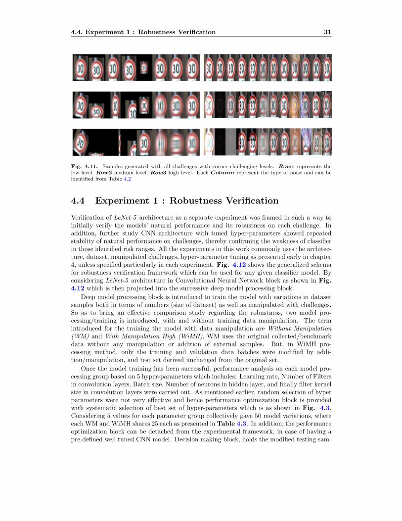
4.11 Samples generated with all challenges with corner challenging levels. Row1
represents the low level, Row2 medium level, Row3 high level. Each Column
represent the type of noise and can be identified from Table 4.2 . . . . . . . . 31
4.12 Generalized robustness verification framework for traffic sign classification . . 32
4.13 Training and validation accuracy for German Traffic Sign Recognition Bench-
mark with only Fk hyper-parameter group . . . . . . . . . . . . . . . . . . . . 35
4.14 Testing accuracy based on two training group along with selected 5 best
set of parameters on each challenge type. Solid line from With Manipulation
clearly outperformed the dotted lines Without Manipulation in extreme levels
of difficulty . . . . . . . . . . . . . . . . . . . . . . . . . . . . . . . . . . . . . 37
4.15 Threshold accuracy based safe-risk range distribution. 20 challenge types
were grouped into Camera orientation, Distance, Occlusion, Blur, Illumina-
tion, and Weather variations. Selected model training with hyper-parameter
are Without Manipulation (WM) and Filter Kernel (Fk) group with 7 3 value 42
4.16 Comparative trained model performance on Occlusion challenge type with
different data augmentation, where Without augmentation (WoA), Random
Augmentation (RA), Predictive Augmentation (PA), and Predictive Multiple
Augmentation (PMA) . . . . . . . . . . . . . . . . . . . . . . . . . . . . . . . 45
4.17 Comparative overall accuracy based on augmentation in testing group, where
Without augmentation (WoA), Random Augmentation (RA), Predictive Aug-
mentation (PA), and Predictive Multiple Augmentation (PMA). The PA and
PMA has got improvement in all five testing groups . . . . . . . . . . . . . . 47
4.18 Comparative confidence based on augmentation in testing group, where With-
out augmentation (WoA), Random Augmentation (RA), Predictive Augmen-
tation (PA), and Predictive Multiple Augmentation (PMA). The PA and
PMA has got improvement in all five testing groups . . . . . . . . . . . . . . 48
5.1 Fall in recognition accuracy for Darkness challenge type based on repeated
augmentation without prior knowledge in model capacity. Dotted lines rep-
resent the model trained without augmentation and the solid lines represent
with augmentation . . . . . . . . . . . . . . . . . . . . . . . . . . . . . . . . . 50

xii LIST OF FIGURES

List of Tables
4.1 Number of image samples used for training, testing and validation present in
each dataset . . . . . . . . . . . . . . . . . . . . . . . . . . . . . . . . . . . . . 26
4.2 Generated Real-Time challenges covering extreme difficulty levels which were
grouped into vehicle and environment perspective . . . . . . . . . . . . . . . . 28
4.3 Training (TR), Validation (VA), and Testing (TE) accuracy on Without
manipulation (WM) and With manipulation high (WiMH) based on hyper
paramter selection. . . . . . . . . . . . . . . . . . . . . . . . . . . . . . . . . . 33
4.4 The results for identified Safe-Risk ranges . . . . . . . . . . . . . . . . . . . . 39
4.5 The results of top performance based on hyper parameters selection. Lr, Fd,
D, B, Fk being Learning rate, Filter depth, Nodes in hidden layers, Batch
size, and Filter kernel size respectively . . . . . . . . . . . . . . . . . . . . . . 39
4.6 Number of image samples for model training and inferencing. Without Aug-
mentation (WoA), Random Augmentation (RA), Predictive Augmentation
(PA) and Predictive Multiple Augmentation (PMA) . . . . . . . . . . . . . . 43
4.7 The results for average safe range accuracy based on augmentation, where
Without augmentation (WoA), Random Augmentation (RA), Predictive Aug-
mentation (PA), and Predictive Multiple Augmentation (PMA), and German
Traffic Sign Recognition Benchmark (GTSRB) . . . . . . . . . . . . . . . . . 44
4.8 The results for average risk range accuracy based on augmentation, where
Without augmentation (WoA), Random Augmentation (RA), Predictive Aug-
mentation (PA), Predictive Multiple Augmentation (PMA), and German
Traffic Sign Recognition Benchmark (GTSRB) . . . . . . . . . . . . . . . . . 46
xiii

xiv LIST OF TABLES

List of Abbreviations
AI Artificial Intelligence
AV Autonomous Vehicles
ADAS Advanced Driver Assistance Systems
SAE Society of Automotive Engineers
TSR Traffic Sign Recognition
ML Machine Learning
DL Deep Learning
GPU Graphical Processing Unit
CNN Convolutional Neural Network
GTSRB German Traffic Sign Recognition Benchmark
BTSD Belgium Traffic Sign Detection
CURE-TSD Challenging Unreal and Real Environments for Traffic Sign Detection
FOV Field of View
PA Predictive Augmentation
PMA Predictive Multiple Augmentation
RA Random Augmentation
WoA Without Augmentation
HOG Histogram of Gradients
VGG Visual Geometry Group
MCDNN Multi Column Deep Neural Network
ANN Artificial Neural Network
FFNN Feed Forward Neural Network
TanH Hyperbolic Tangent
xv
xvi Chapter 0. List of Abbreviations
ReLU Rectified Linear Unit
ELU Exponential Linear Unit
MLP Multi Layered Perceptron
SVM Support Vector Machines
SGD Stochastic Gradient Descent
RMSprop Root Mean Square Propagation
2D & 3D 2 Dimension and 3 Dimension
TR Training
TE Testing
VA Validation
CIELAB International Commission on Illumination
CV Convolution Layer
PL Pooling Layer
FC Fully Connected Layer
DA Data
MH Manipulation High
WM Without Manipulation
WiMH With Manipulation High

Chapter 1
Introduction
Automobiles has seen tremendous growth since 1700s [1] in helping humans move from oneplace to another through sophisticated technologies. Several eras of advancement has beenprevalent with major concentration towards fuel combustion engines, exterior design, utilitypreference, safety and comfort. Furthermore, due to the advancement in the field of elec-tronics [2], sensors, control systems and Artificial intelligence (AI) during early 21st century[3], the automotive sector has pushed their boundaries in providing Advanced Driver Assis-tance Systems (ADAS) [4], autonomous driving functionality [5, 6, 7, 8], lane monitoring [9],etc,. Several research and development are being carried out to achieve level five autonomyaccording to the Society of Automotive Engineers (SAE) standards [10] in automobiles. Atthe same time, safety being a top most priority, such intelligent vehicles are being rigorouslytested in order to adapt to dynamic conditions and cooperate with human driving by shar-ing the road [11, 12, 13, 14, 15]. Among several sensors used in Autonomous Vehicles (AV),camera play a major role in understanding the complex scene around the vehicle in orderto derive necessary information for safer navigation [16]. Since populated urban road envi-ronments are very challenging for an AV, they must satisfy the traffic flow, road signs andrules in regulating the vehicle control. Traffic Sign Recognition (TSR), a computer visionbased algorithm is attracting researchers and automakers in bringing robust classificationirrespective of challenging conditions [17, 18]. However, among many traditional computervision algorithms AI based learning algorithms (i.e. Machine Learning (ML) and DeepLearning (DL)) are preferred as they outperform for TSR [19, 20]. In addition, learningalgorithms are becoming popular nowadays even in complex application due to availabilityof high computing power with the help of Graphical Processing Unit (GPU) even for thecase of huge data requirements [21, 22]. Among various ML and DL models, ConvolutionalNeural Networks (CNN) is widely used for image classification task, which helps in derivingunique features for classifying object of interest of any kind which includes: traffic signs,pedestrians, etc, [19, 23, 24, 25].
1.1 Motivation
A CNN based classifier is a supervised learning model used for recognizing the type ofobject from a given image [24]. This work concentrated on traffic signs as an object ofinterest. Training and performance evaluation of such a model are usually done with thecollected labelled datasets either from real roads or simulation engines. However, generallyavailable labelled datasets, such as German Traffic Sign Recognition Benchmark (GTSRB)
1

2 Chapter 1. Introduction
Fig. 1.1. Experimental camera locations and respective field of view to cover the scene around the vehicle.Based on vehicle size and type, location of cameras are being altered and calibrated.
Fig. 1.2. Image captured from different location on heavy vehicle leads to orientation change in capturedobjects taken from [26]. Left: Front View, Right: Top View
1.1. Motivation 3
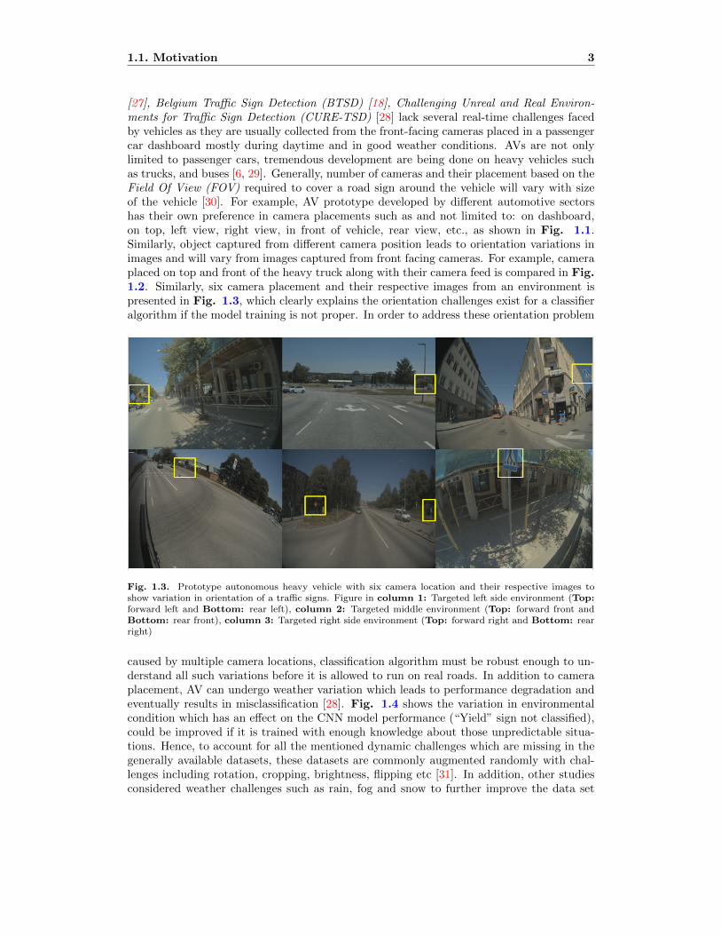
[27], Belgium Traffic Sign Detection (BTSD) [18], Challenging Unreal and Real Environ-ments for Traffic Sign Detection (CURE-TSD) [28] lack several real-time challenges facedby vehicles as they are usually collected from the front-facing cameras placed in a passengercar dashboard mostly during daytime and in good weather conditions. AVs are not onlylimited to passenger cars, tremendous development are being done on heavy vehicles suchas trucks, and buses [6, 29]. Generally, number of cameras and their placement based on theField Of View (FOV) required to cover a road sign around the vehicle will vary with sizeof the vehicle [30]. For example, AV prototype developed by different automotive sectorshas their own preference in camera placements such as and not limited to: on dashboard,on top, left view, right view, in front of vehicle, rear view, etc., as shown in Fig. 1.1.Similarly, object captured from different camera position leads to orientation variations inimages and will vary from images captured from front facing cameras. For example, cameraplaced on top and front of the heavy truck along with their camera feed is compared in Fig.1.2. Similarly, six camera placement and their respective images from an environment ispresented in Fig. 1.3, which clearly explains the orientation challenges exist for a classifieralgorithm if the model training is not proper. In order to address these orientation problem
Fig. 1.3. Prototype autonomous heavy vehicle with six camera location and their respective images toshow variation in orientation of a traffic signs. Figure in column 1: Targeted left side environment (Top:forward left and Bottom: rear left), column 2: Targeted middle environment (Top: forward front andBottom: rear front), column 3: Targeted right side environment (Top: forward right and Bottom: rearright)
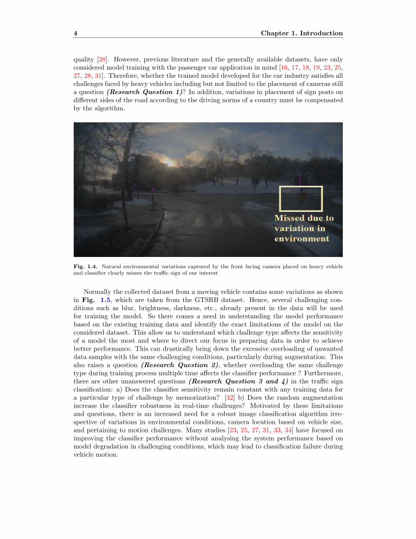
caused by multiple camera locations, classification algorithm must be robust enough to un-derstand all such variations before it is allowed to run on real roads. In addition to cameraplacement, AV can undergo weather variation which leads to performance degradation andeventually results in misclassification [28]. Fig. 1.4 shows the variation in environmentalcondition which has an effect on the CNN model performance (“Yield” sign not classified),could be improved if it is trained with enough knowledge about those unpredictable situa-tions. Hence, to account for all the mentioned dynamic challenges which are missing in thegenerally available datasets, these datasets are commonly augmented randomly with chal-lenges including rotation, cropping, brightness, flipping etc [31]. In addition, other studiesconsidered weather challenges such as rain, fog and snow to further improve the data set
4 Chapter 1. Introduction
quality [28]. However, previous literature and the generally available datasets, have onlyconsidered model training with the passenger car application in mind [16, 17, 18, 19, 23, 25,27, 28, 31]. Therefore, whether the trained model developed for the car industry satisfies allchallenges faced by heavy vehicles including but not limited to the placement of cameras stilla question (Research Question 1)? In addition, variations in placement of sign posts ondifferent sides of the road according to the driving norms of a country must be compensatedby the algorithm.
Fig. 1.4. Natural environmental variations captured by the front facing camera placed on heavy vehicleand classifier clearly misses the traffic sign of our interest
Normally the collected dataset from a moving vehicle contains some variations as shownin Fig. 1.5, which are taken from the GTSRB dataset. Hence, several challenging con-ditions such as blur, brightness, darkness, etc., already present in the data will be usedfor training the model. So there comes a need in understanding the model performancebased on the existing training data and identify the exact limitations of the model on theconsidered dataset. This allow us to understand which challenge type affects the sensitivityof a model the most and where to direct our focus in preparing data in order to achievebetter performance. This can drastically bring down the excessive overloading of unwanteddata samples with the same challenging conditions, particularly during augmentation. Thisalso raises a question (Research Question 2), whether overloading the same challengetype during training process multiple time affects the classifier performance ? Furthermore,there are other unanswered questions (Research Question 3 and 4) in the traffic signclassification: a) Does the classifier sensitivity remain constant with any training data fora particular type of challenge by memorization? [32] b) Does the random augmentationincrease the classifier robustness in real-time challenges? Motivated by these limitationsand questions, there is an increased need for a robust image classification algorithm irre-spective of variations in environmental conditions, camera location based on vehicle size,and pertaining to motion challenges. Many studies [23, 25, 27, 31, 33, 34] have focused onimproving the classifier performance without analysing the system performance based onmodel degradation in challenging conditions, which may lead to classification failure duringvehicle motion.

1.2. Contribution and Scope 5
Fig. 1.5. Natural variations exist in collected GTSRB dataset taken from [27]
1.2 Contribution and Scope
The major contribution of this thesis study is to develop a safety assessment and augmen-tation framework for identification of model capacity negotiating real-time challenges atvarying levels. The framework introduces two new techniques called a Predictive Augmenta-tion (PA) and Predictive Multiple Augmentation (PMA), adapting the dataset for improvedrobustness with high confidence in classifying traffic signs. The trained model based on pro-posed augmentation can withstand variation in camera placement, and weather variationsirrespective of vehicle type and size.
Scope of this work includes,
1. Identification of LeNet-5 classifier weakness with respect to real-time challenges alongwith their corner challenging levels.
2. Generation of 20 different challenge types along with collective 264 levels of difficulty.
3. Consideration of experimental dataset includes: GTSRB and collected data fromheavy vehicle (Scania Autonomous Bus).
4. CNN model training is done based on systematic tuning procedure containing fiveimportant hyper parameters.
5. Performance evaluation based on five testing groups containing real-time challenges.
6. Detailed performance comparison of accuracy and their per-class classification confi-dence for the proposed augmentation methods.

6 Chapter 1. Introduction
1.3 Related Work
Over the last decade, Traffic Sign Recognition (TSR) research has grown rapidly and per-formance in classification accuracy keeps improving [19, 20, 35]. Several algorithms hasbeen developed, right from traditional computer vision techniques to learning models (MLand DL) which are capable of performing classification task in real-time. Traditional clas-sification algorithm such as template matching [36], sliding window method [23], etc., hasa serious disadvantage of higher computational cost and slower performance on real-timeclassification. On the other hand, fundamental ML technique requires hand driven featuresspecifically for each class type during the training process for better understanding the dif-ferent objects. Since, each traffic signs are unique with colour and shape information, handdriven features are made possible based on feature extraction with the help of shape, colour[37], edge [38], Haar feature [23, 39], Histogram of Gradient (HOG) features [23, 20], etc,[40].
In addition to feature extraction, popular classifier algorithms for ML techniques suchas Nearest Neighbour [20, 19], Random Forest [41], Neural Networks [37], Support VectorMachines [42], etc., which are major components in differentiating the class types. However,in the last few years, DL models, a biologically inspired, multilayer architecture based onCNN are increasingly popular due to its high capacity in identifying its own features foreach class type in contrast to ML models. First neural network with CNN architecturehas been developed for binary hand written digit classification with simple two convolutionlayered architecture as LeNet [43]. CNN can vary in network size, which clearly depends onthe complexity of the problem with the help of alternating convolution and pooling layersfor feature extraction.
Followed by the LeNet architecture a variant of CNN, several modified architecturesare being introduced with very deep feature extraction modules particularly for the case,when there are millions of images in training set. State-of-the-art architectures for imageclassification such as VGG [44, 45], ResNet [46], Google net [47], etc., [48] has provided uswith near perfect accuracy scores along with effective generalization over different dataset.Similarly, there are few CNN architecture developed particularly developed for TSR such asLeNet-5 [31], Multi-Column Deep Neural Network (MCDNN) [33, 34], hinge loss model [49],extreme learning [50], etc. Fig. 1.6 shows very deep model developed for general objectclassification task (Google Inception Network) and traffic sign classification task (MCDNN).
To achieve better performance in TSR based on CNN models does not depend only onthe network architecture, there is an increased requirement in using an effective trainingdata itself [51, 52]. Over the past decade, several dataset has been collected with varyingsize, number of class types, challenging environmental conditions, etc [53]. However somedataset are very small and meant only for their personal research, other huge labelled datasetbecomes a benchmark and made universally available. Benchmark dataset are highly suit-able for major computer vision research directions such as object segmentation, detection,classification, etc [27, 18, 28].
Even though several datasets are available, each lack in some features which are notlimited to less number of traffic sign classes, challenging conditions, camera variations, etc.,which are essential to make the algorithm effectively learn and bring robust generalization.Hence, successive labour intensive data collection and labelling has been carried out inorder to eliminate the disadvantages in previously available datasets. Furthermore, gameengines play a major role in generating realistic synthetic dataset according to the userrequirement [28], which can help in compensating the missing traffic sign class types. Severalimage processing techniques are being used in augmenting the images thereby appending

1.3. Related Work 7
the dataset with desired environmental conditions.
(a) Inception Module (GoogleNet Architecture) for object classification taken from [47]
(b) Multi-Column Deep Neural Network for traffic sign classification taken from [33]
Fig. 1.6. State-of-the-art CNN architectures for image classification

8 Chapter 1. Introduction
1.4 Thesis Overview
This thesis is structured in such a way to understand neural networks and their applicationsright from the basics and progressively will answer research questions with results andreasons behind their performance.
– Chapter 2 deals with detailed background on Artificial Neural Networks, buildingblocks of ANN and CNN architecture, and methods followed to manipulate the imagesaccording to the desired noise type.
– Chapter 3 aims at defining the proposed assessment and augmentation frameworkalong with their embedded sub functions.
– Chapter 4 deals with setting up of several experiments derived from the proposedframework in order to answer all our research questions considered in this study in asystematic way.
– Chapter 5 aims at dealing with general discussion based on the achieved results,ways to improve the results, and challenges faced during the study.
– Chapter 6 finally provides summary of this work with major achievements based onthe initial motivations.

Chapter 2
Background & Theory
2.1 Artificial Neural Networks (ANN)
Artificial Neural Networks were developed based on a biologically inspired brains’ neuralactivity, for effectively performing complex task through repeated learning approach withthe help of relevant examples [54, 55, 56]. These examples help the neurons to automati-cally infer rules and features to make decisions. The single neural processing block calleda “Perceptron”, which takes in some input and perform relevant operation to deliver thedesired result. For instance, Perceptron shown in Fig. 2.1 takes multiple inputs and delivera single output, by performing summation of product operation. Multiple Perceptrons con-nected together to form a chained network called Artificial Neurons [56]. Chain connectedANN has been proved to be extremely powerful in wide range of applications particularlyin supervise learning tasks [57]. One such example is a handwritten digit recognition task,which uses several training inputs and their corresponding known labels [43]. ANN performa looped training procedure on each sample till the error between the ground truth labelmatches with the network output. The performance are validated with unknown samples ofsimilar category used in training process. The performance of ANN has tremendously im-proved in later years with enhanced deeper network architecture. The basic building blocksof ANN and their operations are detailed below.
Fig. 2.1. Simple perceptron representation with multi input and single output (solid box as they representconstants). X1...Xn are inputs and W1...Wn are learning weights (hollow box as they represent variables)
9

10 Chapter 2. Background & Theory
2.1.1 Layers
ANN consist of hierarchical layers with systematic connections where information passthrough each Perceptron from one end to other in making final decision [54, 55, 56]. Fig.2.2 shows the simple ANN with connections, where any number of input samples is givenas 1-D feature vector and outputs are defined based on the number of classes (in the case ofclassification) as required by the problem definition. The connections represent the learningweights which varies during the computation process. These adapted weights for each taskrepresent the learned parameter value and can be detached from the network to perform onother similar task without being retrained. The three important layers collectively definesthe ANN architecture, they are Input layer, Hidden Layer and final Output Layer.
Fig. 2.2. Single hidden layer based Artificial Neural Network with 1-D feature vector as input sample andfour class output
Fig. 2.3. Multiple hidden layer based Deep Neural Network (DNN) [58]

2.1. Artificial Neural Networks (ANN) 11
Input Layer : This layer contains only the training samples with single dimension andare connected as shown in Fig. 2.2 with the successive “Hidden Layer” for making simpledecision by summing up the product of input with respective evidence/weights.
Hidden Layer : According to hierarchy, hidden layer will follow the input layer withany number of Perceptron shells, where actual processing of information take place. EachPerceptron shell, which collects the input and their respective weight allocations to calculateweighted sum
∑wixi and make decision based on defined threshold value. Where Xi and
Wi being input and the weight corresponds to ith sample. For example, in binary data, ifthe weighted sum is greater than the threshold, then output throws 1 else 0. Thresholdvalue not necessarily be a constant, it can be non-linear defined based on different “Acti-vation function”, which will be discussed in next section. Both the weights and thresholdvalues used in ANN are real numbers which are very important parameters of a neuron. Forsimple single Feed Forward Neural Network (FFNN), only one hidden layer is used as shownin Fig. 2.2. However, any number of hidden layer along with any number of Perceptronshell can be connected to bring deep network architecture for complex problems as shownin Fig. 2.2. This deeper architecture is represented as “Deep Learning”.
Output Layer : Output Layer can contain any number of output class which will gen-erate only the real numbers according to the problem considered. For example, output witheither 0 or 1 for the case of binary data and can hold range of probabilities for non-binarydata. The probability of each classes can be derived using the loss functions, which will bediscussed later in the section.
Activation Function : Activation function is very important for an Artificial NeuralNetwork for making decisions [59, 48, 49, 58, 24]. Without activation function in Perceptronshell, the output will always be linear in nature as shown in Fig. 2.1. To make senseof something really complicated, there need a Non-linear functional mapping between theinputs and respective output. Simple yet effective Sigmoid functions were used initially todeal the problem of non-linearity in ANN. Sigmoid functions help in achieving boundedactivations within the range [0-1]. However, it has a Vanishing Gradient problem will makethem less effective for deeper networks. For the past decades many other activation functionswere introduced which are considered better based on the complexity of task in bringingdown the computation and thereby increased speed is achieved. Some of the widely usedactivation functions shown in Fig. 2.4 other than Sigmoid are Hyperbolic Tangent (TanH),Rectified Linear Unit (ReLU), Leaky ReLU, Exponential Linear Unit (ELU), Maxout, etc.[59, 60]
Forward and Back Propagation : Generally in ANN, there is a process called For-ward Propagation which help in deriving the network output of class label for a given inputdata with the help of assigned weights [59, 58]. Now, the network output will either be per-fectly matched with the ground truth labels or small error value which has to be minimizedby altering the initial weights, which is done with the help of Back Propagation technique[62]. The back propagation help in finding the partial derivative of error function with re-spect to the weights, thereby help in minimizing error by subtracting with original weightvalues. It is clear that by repeated forward and back propagation ANN learns the inputand gather useful information to activate the desired set of neurons for final results. Thecalculate the difference in error, many loss function has been defined among which Mean-squared error loss function is widely used. Gradient is the derivative of the loss function

12 Chapter 2. Background & Theory
Fig. 2.4. Activation functions for neural networks [61]
with respect to a single weight in each Perceptron, in other words it is simply the slope ofthe function. Powerful gradient descent algorithm [63] is used for updating the weights byminimizing the gradients during backward propagation. However, many development hasbeen achieved in optimizing and speeding the gradient descent procedure (See section 2.2.5).The general schema of the gradient descent algorithm is shown in Fig. 2.5.
Fig. 2.5. Schema of weight flow in gradient descent algorithm, targeted to bring initialized weight to globalminimum [64]
2.2 Convolutional Neural Network (CNN)
The Convolutional Neural Networks is very popular in the field of computer vision par-ticularly in image understanding task [24, 59]. CNN is derived from the traditional ANNand effectively modified according to the vision problems and are employed in several fieldsincluding autonomous driving, medical image analysis, etc [19, 48, 59]. CNN perform betterand are robust in image classification due to their unique feature learning capacity fromhuge training examples compared to the traditional computer vision algorithms. The gen-eral CNN architecture consists of two major functional modules, i.e. feature learning &extraction module and final classification module [50, 65, 49, 59]. CNN is structured with

2.2. Convolutional Neural Network (CNN) 13
three main layers namely convolution layer, pooling layer, and fully connected layer. Thesystematic feature learning module is composed of alternating convolution and pooling lay-ers along with desired activation functions. According to the complexity of the task, thenumber of layers can be increased in feature learning & extraction. Final classification mod-ule is same as that of ANN with Multi-layered Perceptron (MLP) contains desired numberof hidden layers [66]. Similar to ANN, 1) forward propagation 2) back propagation processtake place in feature extraction. The detailed operation of the CNN layers are discussedbelow.
2.2.1 Convolution Layer
Convolution layer is the first layer in CNN architecture which helps in achieving 2-D/3-Dconvolution operation on the input images [24, 59]. Convolution operation provides us withpixel wise weight estimation of an image for the respective filter kernel. This operation isperformed simultaneously on all the channels of the input image and change of weights in 3channels will be collectively recorded in the single channel feature map output . Convolutionoperation has got three main advantages: 1) Since there is a weight sharing ability in thefeature maps, which can effectively reduce the number of parameters to learn 2) Helps inlearning correlation between the neighbouring pixels 3) identifying features invariant to thelocation in an image. The output feature map size generated by the convolution layer canbe controlled with the help of filter kernel size, stride length, and zero padding on inputimages. The convolution operation with single filter kernel Cf provide us with 2D featuremap output image O(m∗n) and is given in the Equation 2.1.
O(m∗n) = I(m∗n∗c) ∗ Cf (m∗n∗c) + b(1∗1∗1) (2.1)
Where m,n,and c are the width,height and channel of the Input image I, output image Oand filter kernel Cf . b is the bias value.
Filter kernel weight matrix Cf dimensions can be varied by stacking more number oflayers for better feature learning. The size of the output map generated by the convolutionlayer can be define by Equation 2.2.
Om = (Im − F + 2P )/S + 1 (2.2)
Where F is the filter kernel dimension, S is the stride length for the sliding window operation,P is the zero padding value which helps to retain the output size of the feature map to thatof input for stride S = 1, Im is the width of input feature map. In case of necessity, theoutput map size can be fixed similar to that of input map size by modifying padding valuewith P = (F − 1)/2.
2.2.2 Pooling Layer
Pooling layer will follow the convolution layer in the CNN architecture. Similar to convo-lution layer, pooling layer provide translational invariant result as they consider the neigh-bouring pixels for their calculation. Pooling layer helps in reducing the spatial sample size ofinput feature map based on overlapping square Max kernels Mk(height∗width). Generally,Max or Average pooling will work in sliding window concept to get the maximum pixel valueby ignoring the smaller ones. On the other hand, average pooling will average the values inthe 9 pixels window to generate the new feature value. Normally, in this layer stride lengthof S = 2 will be considered and without zero padding. The same Equation 2.2 is used tofind the size of the output feature map for pooling layer [50, 65, 49, 59].

14 Chapter 2. Background & Theory
2.2.3 Fully Connected Layer
As mentioned earlier, final classification module holds the MLP layers similar to the ANN inclassifying objects according to the learned features. The simple and complex fully connectedlayers based on inputs which are derived from the final pooling layer output, i.e. 2-D featuremap is concatenated into 1-D vector shown in Fig. 2.2 and 2.3. In addition, non-linearactivation functions as shown in Fig. 2.4 are used in both convolution and fully connectedlayers to fire the neurons.
2.2.4 Loss Function
Generally, loss function aim in assigning high score value for the correct class type comparedto the incorrect classes. The famous classifiers used in CNNs are Multiclass Support VectorMachines (SVM) or Softmax classifier along with their unique loss function representations[58, 59]. The SVM loss function helps in finding the class score with a fixed margin δ aspresented in Equation 2.3 [58]. Summation of all such class loss scores, the SVM lossfunction will assign a final score which corresponds to a class label defined in the task.
Li =∑cj 6=yi
max(0, Fscj − Fsyi + δ) (2.3)
Where Li in Equation 2.3 is the SVM loss value for the ith image by summing all theclass scores. yi is the known class label for the ith image. Fscj and Fsyi are the score function
for the incorrect class and true class type obtained from the linear classifier respectively. δis the fixed margin value which helps in maintaining the score of the correct classes at leastlarger than its own value. The loss function for full training samples can be presented inthe Equation 2.4
L =1
N
N∑i=1
Li (2.4)
Where N is the total number of images in the dataset. Similarly, Softmax classifier whichuses the same loss score calculation for whole training samples is presented in Equation 2.4but with different loss function [58]. Softmax classifier helps us to visualize more intuitivescore values of each class type in terms of normalized probabilities. The loss functionexpression used by Softmax classifier is given by Equation 2.5.
Li = −log
(eFsyi∑cj e
Fscj
)(2.5)
2.2.5 Optimization
Gradient Descent algorithm discussed earlier in section 3.1, which is used for updating theweights in a direction close to global minimum in CNN architecture for learning trainingexamples. There are some advancements in gradient descent algorithm to improve theirperformance and stability which includes, Batch Gradient Descent, Stochastic Gradient De-scent (SGD), and Mini-Batch Gradient Descent [58, 59]. Vanilla or Batch Gradient Descent,computes the gradient of a cost function with respect to the parameters considering the en-tire training samples. Stochastic gradient descent on the other hand performs a parameter

2.3. Image Manipulation 15
update based only on one training example. Furthermore, Mini-batch gradient descent per-forms an update for every mini-batch of n training examples. Still these algorithms hasto be optimized in better way to achieve effective results with less computational power.Learning rate is an important parameter to bring down the computation of optimizer algo-rithm. However, it is quiet challenging to define exact value for learning rate as small valueleads to longer convergence time and vice versa. Hence, several optimizer uses additionalparameters such as momentum, RMSprop, Adam, etc. [58], for better convergence. Adamoptimizer [67], being widely used nowadays for image recognition, with initialized randomsearch for N number of iterations. In addition, among other techniques, Adam uses SGDas their gradient estimation algorithm to optimize the direction of updating weights.
2.3 Image Manipulation
Generally, gathered 2D camera data from moving vehicle in real roads for the purpose oftraining machine learning models does not holds all challenges due to limitation in drivingarea, weather conditions, scene with multiple sign types, road conditions, etc. To accom-modate most of the challenges particularly during the data collection, will increase thelabour cost and unpredictable time line in waiting for the exact conditions to occur in realtime. For example, waiting time for change in monsoon and seasons. These challengesare commonly manipulated using filter kernels from predefined image processing librariesor specially defined filter for each type [68, 69, 70]. This generation helps us in bringingeffective background analysis of how far the classifier can withstand the challenges. Thedetailed set of off-line challenges manipulation process using image processing techniqueswere presented below.
Roll : The decision made by the autonomous vehicles varies with the perspective changesin the images which are caused either by camera angle or tilted/damaged signs from theenvironment during vehicle motion, which can lead to considerable rotation of 2D cameraimages. As, object of interest is in 3D and is projected onto 2D images, we term rotationof images as “Roll” rather than representing with usual literature based name “Rotation”,which greatly helps in correlating other view point challenge type considered in the study.The Fig. 2.6 helps us to understand better how Roll challenge is manipulated on theimage and its extreme ranges along both the directions. The rolling of clockwise and anti-clockwise in images are represented by negative angles and positive angles respectively.Mathematically, Rolling Transformation matrix TR presented in matrix Equation 2.6 takesθ as input and get convoluted with the input image in generating the Roll challenge asrequired without scaling [71]. Rolling Scaling Transformation matrix TRS including desiredscaling is presented in matrix Equation 2.7. Where α = Scale.cosθ, β = Scale.sinθ, Scaleis a scaling factor ranges between [0 - 1], centerX and centerY defines the X & Y coordinateof an image from where it is rotated.
TR =
[cosθ −sinθsinθ cosθ
](2.6)
TRS =
[α −β (1− α).centerX − β.centerYβ α β.(centerX) + (1− α).centerY
](2.7)
Pitch : 3D object of interest from environment can either be viewed from top or bot-tom angle in heavy vehicles, which leads to non-parallel projection of images with respect

16 Chapter 2. Background & Theory
Fig. 2.6. Rolling variation of image can be generated both in clockwise and anti-clockwise direction withdefined angles
to camera plane. In addition, particularly trucks has got heavy suspension in the cabincan also contribute to “Pitch” effect with varying angles as shown in Fig. 2.7. Generally,the pitching effect in an image can be achieved by projective transformations, also knownas a perspective transform or homography [71]. This action operates on homogeneous co-ordinates, where two sets of 4 XY coordinate points are needed from image, first set ofpoints which is to be mapped/projected to get the next set of reference points. These 8pairs of coordinates helps in finding the unknown homographic transformation matrix using8 equations as presented in matrix Equation 2.9. The mathematical representation ofprojective transformation is presented in Equation 2.8, where H refers to the 3*3 homo-geneous transformation matrix, where Ix,y,1 refers to the input image and I
′
x,y,1 belongsto projected output image. The projective transformation based on XY coordinates aremapped in terms of angle variation θ for this work and will be discussed later in section.
I′
x,y,1 = H.Ix,y,1 (2.8)
H =
H11 H12 H13
H21 H22 H23
H31 H32 1
(2.9)
I′
x,y = A.Ix,y (2.10)
A =
[A11 A12 A13
A21 A22 A23
](2.11)
Yaw : Similar to Pitch variations, object of interest might occur in orthographic pro-jection with respect to vehicle front view and leads to “Yaw” effect in images along with

2.3. Image Manipulation 17
Fig. 2.7. Pitch variation of image can be generatedin order compensate the Top and Bottom view of anobject
Fig. 2.8. Yaw variation of image can be generated inorder compensate the view from Left and Right sideof an object
varying angles as shown in Fig. 2.8. Generally, orthographic projections or Multiview pro-jections are generated with the help of Affine transformations [71], which requires two setsof 3 XY coordinate points, where first set belongs to points which is to be projected to getthe next set of reference points. These 6 pairs of XY coordinate helps in finding the variablesin Affine transformation matrix presented in Equation 2.10, which is then convoluted withthe any input image pixels to achieve desired transformation. The mathematical represen-tation of Affine transformation is presented in Equation 2.10, where A refers to the 2*3transformation matrix, where Ix,y refers to the input image and I
′
x,y belongs to transformedoutput image. The Affine transformation based on XY coordinates are mapped in terms ofangle variation θ for this work and will be discussed later in section.
Occlusion : Occlusion is one of the important challenge naturally occur when informa-tion is perceived from the environment, where part of the desired object will be overlappedby an undesired object. In addition, sometimes object detector may crop the part of anobject, which is necessary for classification resulting in wrong identification. The Fig. 2.9helps us to understand better the simple occlusion challenge that can occur in an image.Generation of occlusion can be done using linear translation of image data from a fixed co-ordinates, thereby achieving part of the useful information about the object of interest [71].The image translation is presented in the Equation 2.12. Where L being the transfor-mation matrix for translation as presented in the matrix Equation 2.13, where Ix,y refers
to the input image and I′
x,y belongs to translated output image with transX and transYbeing translational value in X and Y coordinates respectively [69, 70].
I′
x,y = L.Ix,y (2.12)

18 Chapter 2. Background & Theory
L =
[1 0 transX0 1 transY
](2.13)
Fig. 2.9. Occlusion variation of image can be generated in order compensate the changes occurring in anypart of an object
Distance : It is very important for the vision algorithm to take quick action once itperceive information from the real world. The system can either be developed with highspeed recognition in close range or must make decision from long ranges. It is encouragedthat long range identification will be effective and necessary even if the system is capable ofhigh speed close range performance for safer navigation. The Fig. 2.10 shows the variationsin image dimension from short to long distance ranges. Since the CNN considered in thiswork does not allow for varying input image size, image data will be surrounded/padded byblack pixels to match the defined dimension [71]. It is worth mentioning, the black pixelpadded will be thrown away by activation function during feature extraction stage in CNNmodels. The generation of small to large size images with padded black pixels are presentedin Equation 2.14. Where S being the transformation matrix for scaling as presented inthe matrix Equation 2.15, where Ix,y refers to the input image and I
′
x,y belongs to scaledoutput image with Sx and Sy being scaling factor in X and Y coordinates respectively andrange between [ 0 - 1 ]. Later this scaled image is then merged with the black image ofdesired dimension.
I′
x,y = S.Ix,y (2.14)
S =
[Sx 00 Sy
](2.15)
Motion Blur : Motion of speeding vehicle in the real road, introduces different blurringeffect notably the frames captured with shakes caused due to rigid fixing of cameras. Theuneven road surfaces like ups and downs introduces motion blur in vertical direction, fastmotion of vehicle in horizontal direction leads to blur in horizontal direction and finally lenszooming/focus leads to random Gaussian lens blur. The mathematical filter kernel used togenerate Horizontal Blur HB is given in matrix Equation 2.16 which is then convolutedwith the original image [71]. It works like a directional low pass filter which averages thepixel value in desired direction [69, 70]. Similarly, filter kernel used to generate VerticalBlur VB is given in the matrix Equation 2.17. The Gaussian blur GB can be considered
2.3. Image Manipulation 19
Fig. 2.10. Distance variation of image can be generated from short to long ranges
as a low pass filter which attenuates the high frequencies in the image and causes blurringeffect with the help of defined standard deviation value in both x and y direction as givenin the Equation 2.18.
HB =
0 0 01 1 10 0 0
(2.16)
VB =
0 1 00 1 00 1 0
(2.17)
GB(x, y) = 1/(2πσ2)e−(x2+y2)/2σ2
(2.18)
Illuminations : The perceived images from the environment will undergo differentillumination conditions which may leads to excessive brightness, darkness and contrast vari-ations. To account for these challenges, input training samples to the classifier, wherecontrast variation is generated with the help of a α factor as presented in the Equation2.19. Where C(x, y) is the contrasted output image with α > 0 being the factor in choosingthe strength of contrasting level, I(x, y) being the input image to be manipulated, and βbeing brightness parameter, which is kept constant as value 0 for this contrast variation op-eration. For the brightness and darkness improvement in the input images, following gammacorrection as presented in Equation 2.20 is used, where B(x, y) and D(x, y) brightenedand darkened output image respectively. When there is γ > 1 and γ < 1, brightness anddarkness effects are achieved respectively. here can be a case where shadow effect falls on theobject of interest both in vertical and horizontal direction, hence band gamma correctionwith darkness parameter can be used as shown in Fig. 2.11 [69, 70].
C(x, y) = α.I(x, y) + β (2.19)
B(x, y), D(x, y) = (I(x, y)/255)γ ∗ 255 (2.20)
Blending Challenge : In addition to the above mentioned challenges, caused due tovehicle motions, view point, hardware and poor lighting conditions, object recognition hasalso got additional variations caused due to the natural weather changes. For example,

20 Chapter 2. Background & Theory
Fig. 2.11. Shadow variation can be generated both in horizontal and vertical direction of an object
snowflakes falls on the object and the resulting perceived image will have overlapped objectof interest and snowflakes, like blending effect. Generally, image blending operation iscarried out with the help of reference filter image on top of the original colour image (R;G; B; A). In this operation, the final alpha channel ‘A’ defines the opacity of the imagedata and plays a major role in achieving blending effect as mentioned in the mathematicalEquation 2.21. Where α is the blending factor of two images and its value ranges between[0 - 1], I1(x, y) & I2(x, y) refers to input and filter images to be blended respectively, andBlendout is the desired output image. The Fig. 2.12 presents a visualization example ofblending operation.
Blendout = I1(x, y) ∗ (1.0− α) + I2(x, y) ∗ α (2.21)
Fig. 2.12. Blending of two input images in order to create overlapping challenges on one image

Chapter 3
Assessment and AugmentationMethod
Motivated by the classifier degradation, particularly caused due to real-time challenges facedby the moving vehicles, this thesis work proposes a Safety-Risk assessment and augmentationframework. In addition to the framework, two specific augmentation techniques were intro-duced namely Predictive Augmentation (PA) and Predictive Multiple Augmentation (PMA)for effective CNN model training. Proposed framework and two augmentation techniqueswill deliver a concrete solution in adapting the CNN model to withstand the degradationcaused by the challenging conditions. Detailed description of the proposed framework ispresented below.
3.1 Safety-Risk Assessment and Augmentation Frame-work
Fig. 3.1 shows the detailed flow chart of proposed safety-risk assessment and improvisa-tion framework for traffic signs with one challenging sample performance before and afterframework processing. Detailed description of two sub platforms defined in the proposedframework were presented in this section. As this study focuses on understanding theclassifier capacity on challenges before being deployed into real systems, initial safety-riskverification is of prime importance. Then model training can be adapted as per the require-ments needed by the classifier to improve its performance. Hence, the framework is dividedinto two sub platforms called, 1) Safe-Risk Assessment, which helps in identifying the classi-fier weakness on each considered challenge type 2) Predictive Augmentation, which helps inincreasing the training sample needed by the CNN model to understand the challenge typewhich falls under their weakness. The framework is developed to handle any given classifiermodel to understand their capacity based on our requirements. Selected CNN architecturealong with their dataset (training, testing and validation batches) are the only requirementsfor this framework. Similar to robustness framework, best performing CNN model has beenselected to verify their capacity based on tuning hyper-parameters for the given data (SeeChapter 4). Detailed description regarding two major platforms were discussed as follows.
21

22 Chapter 3. Assessment and Augmentation Method
Fig. 3.1. Schematic flow chart to represent the Safety-Risk assessment and augmentation frameworkfor traffic sign classification with training (TR), validation (VR), and testing (TE) being the input data.Identified weakness in terms of challenge type and its difficulty level (Risk Ranges) are used by the predictiveaugmentation platform to improve the training and validation samples

3.1. Safety-Risk Assessment and Augmentation Framework 23
3.1.1 Safe-Risk Assessment
Safe-Risk Assessment platform presented in the framework as shown in Fig. 3.1 helpsin quantifying the model capacity for each challenge type. As discussed earlier, the bestperforming traffic sign classifier algorithm and its dataset used for training (TR), validation(VA) and testing (TE) were the only input requirement for the assessment platform. Eventhough the input CNN model is claimed to be best performing for testing samples, majoraim of this proposed framework is to validate their performance on challenging conditionsand retrain the model according to the systematic hyper-parameter tuning procedure (Seesection ) to validate its stability.
Hyper-parameter tuning and retraining take place inside CNN model tuning & trainingpresented in framework. In order to understand their performance and robustness on real-time challenges faced by the vehicles, Real-time challenge generation block is equipped withan array of challenges (filter kernels) which are then manipulated on top of the derivedtesting samples (See Section 4.3) from the input dataset.
Fig. 3.1 clearly shows a test sample with pitching challenge type is misclassified withhigh confidence even with the considered best performing classifier. Hence, a Safe & RiskRange Identification block helps in identifying the challenge type and their difficulty levelswhich were mostly misclassified by the classifier and requires respective training samplesfor better classification. The procedural way to select the safe and risk ranges for eachchallenge type has been formulated based on threshold recognition accuracy as shown inFig. 3.2. As generalized identification has to be achieved, all considered challenges weregrouped into symmetric and linear types as shown in Fig. 3.2 with low being qualitativelyless challenging and high being more challenging (See section). If the classification accuracyfor considered challenge type and difficulty level reaches above the defined threshold level,then those will falls under safe ranges and vice versa. Threshold accuracy for identificationcan be defined based on the requirements that how good the classifier should perform inthe wild. As this platform gave a detailed intuition about targeting the data batch withchallenges for future model training. Identified limitation in terms of Risk ranges for eachchallenge type is fed as input to the successive predictive augmentation platform.
3.1.2 Predictive Augmentation
Predictive Augmentation (PA) platform being the second part of framework has been in-troduced to improve the previously available training samples with real-time challenges.Augmentation were done based on the predicted challenges along with their risk rangeswhich were gathered from previous safe-risk assessment platform. Since augmentation car-ried out based on the identified model capacity, improvement in performance and robustnesshas been achieved as shown in Fig. 3.1. Those identified limitations are augmented onthe training samples in two different ways, they are : 1) PA, which used only one identifiedchallenge to augment the test image. For example, a speed limit 30 km/hour with a (blur)difficulty level 10. So, the next sample will contain a different challenge type and level; 2)PMA, on the other hand, uses two variations, one was a challenge type from an identifiedrange and the other was a CIELAB colour space due to its high feature learning capacity[65] so as to bring simultaneous overlapped effect of both on the same image. This helpsthe classifier model to understand the combined variations occurring in the environment.

24 Chapter 3. Assessment and Augmentation Method
(a) Linear challenge type
(b) Symmetric challenge type
Fig. 3.2. Systematic selection of safe and risk ranges based on defined threshold recognition accuracy foreach challenge type

Chapter 4
Experiments
This chapter presents the detailed insight on general dataset selection, CNN architectureselection, generation of challenge for augmentation and validation commonly shared betweenthe experiments, and finally three stages of experimentation were framed in order to coverthe sub processes proposed in the framework. Finally, results achieved and their performancewere evaluated.
4.1 Dataset Selection
To validate the proposed frameworks, two dataset were considered. 1) German Traffic SignRecognition Benchmark (GTSRB) data, and 2) collection of own 2D camera data from ex-perimental autonomous bus navigated in urban Swedish roads as shown in Fig. 4.1
GTSRB : GTSRB data were mainly considered for this study as most of the traffic signdetection, classification and tracking algorithm has been bench-marked as well as they werecollected from physical real-world German roads. The data samples has been collected as avideo sequence for approximately 10 hours recorded with a camera placed on dashboard ofa passenger car while driving in urban road environment (Germany) only during daytime.GTSRB dataset was compiled with final data size of 50000 images with 43 different classes.The dataset contains images of more than 1,700 traffic sign instances along with the imagesize which varies between 15 * 15 and 222 * 193 pixels dimensions. To make uniform inputto the classifier all the images are resized to 32*32 dimensions [27]. The Table 4.1 sharesmore information on training, validation and testing image samples used for this study. Fig.4.1 shows batch of sample images from GTSRB, which were presented in the left side.
Heavy vehicle Data: According to the motivation presented in introduction chapter,dataset collection were done from autonomous bus to show the variations in images com-paring heavy vehicle with passenger car data. The data collected were from monocularcamera, which was placed centred inside the cabin. The camera was placed in a positionwhich was high from the ground compared to the usual camera location in passenger cars.This greatly helped in understanding the necessity of training data and the performancewith respect to high angle camera placement. In addition, some environmental conditionslike darkness, brightness, etc,. were captured from the scene in Swedish roads. Collectedheavy vehicle data were comparatively very small with only 4 sign types which includes“Pedestrian crossing”,“Yield”, “Traffic light red”, and “Keep right”. We used only 4 sign
25

26 Chapter 4. Experiments
Fig. 4.1. Sample images collected from dataset considered for this study with natural variations. Left:German Traffic Sign Recognition Benchmark Right: Collected heavy vehicle data with four class types
types as these were the maximum number of samples captured. In addition, the small datasize helps us to bring an effective measure to prove our claim that predictive augmentationwill improve irrespective of data size (See Section 4.6.1).
Table 4.1. Number of image samples used for training, testing and validation present ineach dataset
GTSRB Heavy vehicleTrain 34799 161Valid 4410 41Test 12630 51
4.2 CNN Architecture Selection
As the major contribution of this study was to identify the model degradation in order tobring better solution to improve robustness based on augmentation method, simple CNNarchitecture design was chosen rather than going with deep models. Fig. 4.2 shows thedetailed architecture of considered CNN model for the following experiments. However,the architecture was inspired from “LeNet” binary handwritten character recognition [43],model has been adapted to work on colour images with 3 channel input and some of thehyper parameters were modified in successive systematic tuning procedures. Generally,selection of such hyper parameters were very challenging based on previous studies [31].Hence, rather than utilizing random set of hyper parameter value, this work introduced asimilar procedural way to select best set of values as shown in Fig. 4.3. Five parametergroups were selected, each with 5 different values, collectively gives us 25 set of parametersaccording to our procedure. Tuning begins with initially assigned set of parameters andbest value from each group successively replace the main architecture thereby achievingfinal set of best parameter values. For all the experiments, the above mentioned systematicselection procedure were used. However, for the case of robustness verification, best set ofparameters in each groups were considered for performance comparison. On the other hand,for predictive augmentation experiment only the final set of parameters were considered.

4.2. CNN Architecture Selection 27
Fig. 4.2. CNN Architecture : Input → CV1 → PL1 → CV2 → PL2 → FC1 → FC2 → FC3 (Output).Convolution layer(CV), Polling Layer(PL), Fully connected layer (FC), and feature reduction correspondingto each layer in terms of image dimension is embedded inside blocks
Fig. 4.3. Systematic selection of hyper parameters, with Lr, Fd, D, B, Fk being Learning rate, Filterdepth, Nodes in hidden layers, Batch size, and Filter kernel size respectively

28 Chapter 4. Experiments
4.3 Challenge Generation
Real-time challenges faced by the moving vehicle, irrespective of its vehicle type and size,environmental variation, etc, were generated and grouped into vehicle and environmentperspective category including extreme levels. These extreme levels were considered inorder to bring extensive analysis in identifying the maximum possible sensitivity level ofa considered CNN model. However, the challenge type and their wide range of difficulties(simple to extreme) can be defined based on user requirements before we allow our frameworkto process the input samples. Generally, this helps in removing such ineffective challengelevels for classification task. The detailed set of challenges and their ranges generated werepresented in the Table 4.2. The challenge levels are defined based on the qualitativedegradation effect. Total number of 264 challenge levels from 20 different challenge typescovering most of situations faced by the moving vehicle to mimic the vehicle as in urbanroads, compared to other studies. Some of the challenges were generated using the predefinedfilter kernel available in the image processing toolbox [69, 70], and other environmentalchallenges with three levels were created using defined filters which includes: Snow in Fig.4.4, Rain in Fig. 4.5, Fog in Fig. 4.6, Dust storm in Fig. 4.7 , Smoke in Fig. 4.8,Water flow on windshield in Fig. 4.9, and finally water bubbles either on object or on lensin Fig. 4.10. More theoretical challenge generation of each type on images is presented in(See section 2.3).
Table 4.2. Generated Real-Time challenges covering extreme difficulty levels which weregrouped into vehicle and environment perspective
Challenge Range ChallengesType Min Max Intervals Total(Nos) Units Difficulty
Veh
icle
Per
spec
tive Roll -30 30 2 31 Degree Symmetric
Pitch -90 90 6 31 Degree SymmetricYaw -90 90 6 31 Degree SymmetricOcclusion -14 14 1 29 XY coordinate SymmetricDistance 15 30 1 16 Image Dimension Low-HighMotion Vertical 1 10 1 10 Challenge level Low-HighMotion Horizontal 1 10 1 10 Challenge level Low-HighGaussian Blur 1 10 1 10 Challenge level Low-High
Envir
onm
ent
Per
spec
tive
Brightness 1 15 1 15 Challenge Level Low-HighDarkness 1 15 1 15 Challenge Level Low-HighContrast 1 15 1 15 Challenge Level Low-HighShadow Vertical 1 15 1 15 Challenge Level Low-HighShadow Horizontal 1 15 1 15 Challenge Level Low-HighFog Low High Medium 3 Challenge Level Low-HighRain Low High Medium 3 Challenge Level Low-HighSnow Low High Medium 3 Challenge Level Low-HighDust Low High Medium 3 Challenge Level Low-HighSmoke Low High Medium 3 Challenge Level Low-HighWater Low High Medium 3 Challenge Level Low-HighBubbles Low High Medium 3 Challenge Level Low-High
4.3. Challenge Generation 29
Fig. 4.4. Filter kernel used to generate “Snow” flakes on images with less to more number of flakes perimage
Fig. 4.5. Filter kernel used to generate “Rain” strokes on images with horizontal and angled presence perimage
Fig. 4.6. Filter kernel used to generate “Fog” on images with low to high dense cloud per image

30 Chapter 4. Experiments
Fig. 4.7. Filter kernel used to generate “Dust” on images with low to high dense of dust particles perimage
Fig. 4.8. Filter kernel used to generate “Smoke” on images with low to high dense fumes per image
Fig. 4.9. Filter kernel used to generate “Water Flow” on images with low to high variation per image
Fig. 4.10. Filter kernel used to generate “Bubble” on images with small to large bubble size per image
4.4. Experiment 1 : Robustness Verification 31
Fig. 4.11. Samples generated with all challenges with corner challenging levels. Row1 represents thelow level, Row2 medium level, Row3 high level. Each Column represent the type of noise and can beidentified from Table 4.2
4.4 Experiment 1 : Robustness Verification
Verification of LeNet-5 architecture as a separate experiment was framed in such a way toinitially verify the models’ natural performance and its robustness on each challenge. Inaddition, further study CNN architecture with tuned hyper-parameters showed repeatedstability of natural performance on challenges, thereby confirming the weakness of classifierin those identified risk ranges. All the experiments in this work commonly uses the architec-ture, dataset, manipulated challenges, hyper-parameter tuning as presented early in chapter4, unless specified particularly in each experiment. Fig. 4.12 shows the generalized schemafor robustness verification framework which can be used for any given classifier model. Byconsidering LeNet-5 architecture in Convolutional Neural Network block as shown in Fig.4.12 which is then projected into the successive deep model processing block.
Deep model processing block is introduced to train the model with variations in datasetsamples both in terms of numbers (size of dataset) as well as manipulated with challenges.So as to bring an effective comparison study regarding the robustness, two model pro-cessing/training is introduced, with and without training data manipulation. The termintroduced for the training the model with data manipulation are Without Manipulation(WM) and With Manipulation High (WiMH). WM uses the original collected/benchmarkdata without any manipulation or addition of external samples. But, in WiMH pro-cessing method, only the training and validation data batches were modified by addi-tion/manipulation, and test set derived unchanged from the original set.
Once the model training has been successful, performance analysis on each model pro-cessing group based on 5 hyper-parameters which includes: Learning rate, Number of Filtersin convolution layers, Batch size, Number of neurons in hidden layer, and finally filter kernelsize in convolution layers were carried out. As mentioned earlier, random selection of hyperparameters were not very effective and hence performance optimization block is providedwith systematic selection of best set of hyper-parameters which is as shown in Fig. 4.3.Considering 5 values for each parameter group collectively gave 50 model variations, whereeach WM and WiMH shares 25 each as presented in Table 4.3. In addition, the performanceoptimization block can be detached from the experimental framework, in case of having apre-defined well tuned CNN model. Decision making block, holds the modified testing sam-

32 Chapter 4. Experiments
Fig. 4.12. Generalized robustness verification framework for traffic sign classification

4.4. Experiment 1 : Robustness Verification 33
ples with all the challenges in every difficulty level. Verification were done only on theGTSRB data with WM as presented in Table 4.1, and for WiMH the number of sampleswere double the size in each training, validation and testing. Interesting to note that thisexperiment has revealed the behavioural changes either degradation/improvement/stabilityin each model through different manipulated training batches.
Table 4.3. Training (TR), Validation (VA), and Testing (TE) accuracy on Without ma-nipulation (WM) and With manipulation high (WiMH) based on hyper paramter selection.
Hyper Parameter WM Accuracy (Epoch 30) WiMH Accuracy (Epoch 50)Group Value TR VA TE TR VA TE
Lr
0.01 5.7 5.4 5.9 3.0 3.2 5.50.001 99.1 99.4 91.6 83 63 84.10.0001 99.8 99.8 91.6 89 61 85.60.0005 99.5 99.2 93.4 91 66 880.00005 99.8 99.8 90.4 81 55 81.8
Fd
12,32 99.5 99.5 93.8 96 71 90.624,64 99.5 99.6 94.6 95.5 74.4 91.848,128 99.5 99.3 93.1 95.8 75.8 92.296,256 99.6 99.6 94.2 96 73 93.3192,512 99.9 99.9 94.8 93 72 90.2
D
100,50 5.7 5.45 5.9 3.2 3.35 5.6200,120 99.7 99.7 95.6 97 74 93.2256,100 99.8 99.6 95.2 92 69 93300,200 99.8 99.5 94.4 95 69 92.3300,256 99.2 99.4 93.3 96 71 92.3
B
48 99.8 99.8 92.4 96.2 74 93.164 99.6 99.1 93.8 95.4 71 92.8100 99.6 99.5 95.1 98.1 72 93.5128 99.5 99.5 94.4 99.2 72 91.4256 100 100 95.6 98.4 70 92.4
Fk
3,3 99.9 99.8 92.4 99.2 70 92.13,5 100 100 94.2 96.1 68 89.75,3 100 100 95 98.5 72 93.27,3 100 100 95.5 98.4 75 947,5 99.9 99.9 94.6 98.4 73 93.5
4.4.1 Results
This section reports the results achieved for experiment 1 which were performed only on twomodel processing/training namely,Without Manipulation (WM) and With ManipulationHigh (WiMH) for performance evaluation. As described in the Section 5.2, among theselected set of five hyper parameter group with five values each for LeNet-5 model weretabulated as shown in Table 4.3 in the form of achieved training and validation accuracyfor both WM and WiMH. The epochs are fixed to 30 (WM) and 50 (WiMH) for analysis asbeyond which it reaches saturation limit of performance.
In each parameter group, best performing recognition accuracy were highlighted in theTable 4.3 and they were selected as the final parameter value for model comparison. Basedon such selection process, it helped to boil down to 5 set of model parameters from 25. Thetraining and validation accuracy for WM and WiMH were presented in the form of graphs asshown in Fig. 4.13, but only for Fk parameter group. Similar set of procedure and graphs

34 Chapter 4. Experiments
were followed for other four parameter groups. These graph helped in understanding thevariation in recognition accuracy for each training iteration (Epochs), where WM deliveredsaturated results after 5 iteration and WiMH shows after 25 iterations.
In addition, compared to WM, WiMH showed under-fitting particularly in validationaccuracy which was caused due to manipulation of data samples with real-time challenges.Now, the selected set of 5 models (WM and WiMH trained) were tested on 20 differentchallenge types (Roll to Bubbles) manipulated on testing batches. Each challenge type anddifficulty level were manipulated on all 12630 testing samples and the comparative resultsare plotted in graphs as shown in Fig. 4.14. The testing results were presented only for4 challenge types covering symmetric and linear type for better understanding. All otherresults were added in the appendix A.
It is clearly visible from the graphs that solid lines (WiMH trained models) performedbetter than dotted line (WM trained models) in most of the challenge types particularlyat extreme difficulty levels. In addition, it is clear that challenge with less difficulty hassimilar performance in both WM and WiMH trained models. Hence, concentration on theextreme conditions should be the focus in enhancing the performance in those levels as wellas stabilizing the performance in lower levels. However, very extreme conditions may notbe feasible for classification due to high level of distortion, that can be defined based on therequirements.
These results allowed us to identify the level to which a CNN model can tackle the par-ticular challenge type in real world scenarios. Furthermore, this comparative analysis of 5model parameters in single graph also helped in finding the performance of best parametertuned model among the selected values. In some challenge types like Gaussian blur, Bright-ness and darkness performance of WiMH model does not improve and the reasons will bediscussed later in the discussion section.

4.4. Experiment 1 : Robustness Verification 35
(a) Without Manipulation (WM)
(b) With Manipulation High (WiMH)
Fig. 4.13. Training and validation accuracy for German Traffic Sign Recognition Benchmark with only Fkhyper-parameter group

36 Chapter 4. Experiments
(a) Roll Challenge
(b) Pitch Challenge

4.4. Experiment 1 : Robustness Verification 37
(c) Distance Challenge with usually squared image dimension n*m where n represent the numberof pixels covering height and m represent the number of pixels covering width
(d) Motion Vertical Challenge
Fig. 4.14. Testing accuracy based on two training group along with selected 5 best set of parameterson each challenge type. Solid line from With Manipulation clearly outperformed the dotted lines WithoutManipulation in extreme levels of difficulty

38 Chapter 4. Experiments
4.5 Experiment 2: Model Capacity Identification
Based on the results achieved from robustness verification experiment results, it is clear that,augmenting the training data with real-time challenges has drastically improved the modelperformance even in the corner difficulty levels. However, manipulating whole set of all thechallenges including difficulty levels might lead to over-fitting and increased computationalcost. Hence proposed work target the weakness of the model by initial identification of itscapacity based on each challenge type which were originally collected from training data,so as to exactly quantify the safe and risk ranges for any considered CNN model (SeeSection 3). Both the datasets, GTSRB and Heavy vehicle data were considered for suchcapacity identification with 85% and 75% threshold accuracy for discriminating safe andrisk ranges respectively. The LeNet-5 based CNN architecture is chosen with fine tunedhyper-parameters. Each challenge type and difficulty level is manipulated on all consideredtesting data batches. Hence, 264 difficulty level testing files with each 12630 & 51 samplesfor GTSRB and Heavy vehicle dataset respectively is considered.
4.5.1 Results
We report the results for identified LeNet-5 model capacity (smaller CNN architecture isselected to focus our claims and contribution), where the training data used for modeltraining is without challenge type augmentation. Initial experiments for collected GTSRBand Heavy vehicle data with selected CNN architecture showed the classification accuracyof 96% and 86% respectively (Table 4.5) with the help of the systematic hyper-parameterstuning. It is clear that the two parameter groups (B and Fk) for heavy vehicle data, thehighlighted accuracy in Table 4.5 delivered similar performance. Therefore, the final set ofparameters were selected as, GTSRB data: Lr:5e-4; Fd:192,512; D:200,120; B:256; Fk:7,3;and Heavy vehicle data: Lr:5e-5; Fd:24,64; D:256,100; B:128; Fk:7,3.
The identified safe and risk ranges for each challenge type is clearly depicted in Table4.4 for two different datasets. Since, this study considered 20 challenge types, which weregrouped into six categories to collectively present the safe-risk range selection in Fig. 4.15.
The six categories considered includes: Camera Orientation, Distance, Occlusion, BLur,Illumination, and Weather. The range selection results were presented only for the GTSRBdataset where threshold is fixed as 85%. Similar selection were followed for Heavy vehicledataset.
From the Fig. 4.15, some challenges like Gaussian blur, Darkness, and Brightnessfalls only under the safe ranges. Hence, this result confirms the original data consideredfor model training itself is best enough to perform well in those challenging condition evenin extreme difficulty levels. In addition, it is clearly understandable from Table 4.4 thatwhich challenge type and its difficulty level falls directly in safe ranges. The Fig. 4.15also helps in understanding the stability of the model in each type effectively for furtherimprovisation. The wide range of difficulty levels in each type is spread across X axis ineach figure and the selected risk ranges is used for targeted augmentation in the proposedPA and PMA techniques to improve the classifier robustness. Based on the experimentalresults and analysis, Table 4.4 show that major variations in terms of risk ranges wereseen in camera orientation based challenges, particularly Pitch and Yaw which clearly varywith passenger car and heavy vehicles. This proved our claim 1 where challenges faced bydifferent vehicle can affect classifier performance.

4.5. Experiment 2: Model Capacity Identification 39
Table 4.4. The results for identified Safe-Risk ranges
GTSRB Heavy vehicle
Type Safe Ranges Risk Ranges Safe Ranges Risk Ranges
Roll -14 to 14 -15 to -30 & 15 to 30 -30 to 30 -
Pitch -6 to 6 -12 to -90 & 12 to 90 -24 to 24 -30 to -90 & 30 to 90
Yaw -6 to 6 -12 to -90 & 12 to 90 -18 to 18 -24 to -90 & 24 to 90
Occlusion -1 to 1 -2 to -14 & 2 to 14 -6 to 6 -7 to -14 & 7 to 14
Distance 26 to 30 15 to 25 20 to 30 15 to 19
Motion Vertical 1 to 5 6 to 10 1 to 10 -
Motion Horizontal 1 to 5 6 to 10 1 to 10 -
Gaussian Blur 1 to 10 - 1 to 10 -
Brightness 1 to 13 14 & 15 1 to 15 -
Darkness 1 to 15 - 1 to 15 -
Contrast 1 to 8 9 to 15 1 to 6 7 to 15
Shadow Vertical 1 to 4 5 to 15 1 to 4 5 to 15
Shadow Horizontal 1 to 4 5 to 15 1 to 8 9 to 15
Fog - Low to High - Low to High
Rain - Low to High - Low to High
Snow - Low to High - Low to High
Dust - Low to High - Low to High
Smoke - Low to High - Low to High
Water - Low to High - Low to High
Bubbles - Low to High - Low to High
Table 4.5. The results of top performance based on hyper parameters selection. Lr, Fd,D, B, Fk being Learning rate, Filter depth, Nodes in hidden layers, Batch size, and Filterkernel size respectively
Recognition Accuracy
Dataset Lr Fd D B Fk
GTSRB 93.4 94.7 95.55 95.56 95.6
Heavy Vehicle 86.27 80.4 82.4 86.3 86.3

40 Chapter 4. Experiments
(a) Camera Orientation Variations
(b) Distance Variation

4.5. Experiment 2: Model Capacity Identification 41
(c) Occlusion Variation
(d) Blur Variations
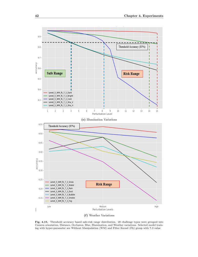
42 Chapter 4. Experiments
(e) Illumination Variations
(f) Weather Variations
Fig. 4.15. Threshold accuracy based safe-risk range distribution. 20 challenge types were grouped intoCamera orientation, Distance, Occlusion, Blur, Illumination, and Weather variations. Selected model train-ing with hyper-parameter are Without Manipulation (WM) and Filter Kernel (Fk) group with 7 3 value

4.6. Experiment 3: Predictive Augmentation 43
4.6 Experiment 3: Predictive Augmentation
This experiment introduced in order to cover the final part of the proposed framework (Pre-dictive Augmentation as in Fig. 3.1) so as to validate the targeted augmentation techniquebased on the identified risk range results derived from experiment 2. The risk ranges foreach challenges were then augmented on the training and validation data batches for train-ing the model. To bring effective comparative analysis, model training is done based onfour different augmentation groups which includes: Without augmentation (WoA), RandomAugmentation (RA), Predictive Augmentation (PA), and Predictive Multiple Augmentation(PMA). WoA refers to no manipulation of challenges in training, validation and testingsamples. RA is augmented as per previous studies for training and validation samples. PAand PMA were augmented based on predicted challenge levels (See Chapter 3) containingsingle and double challenge type on top of the same image [Fig]. In addition to trainingthe model with augmented data, inference has been carried out with five different testinggroup includes: “Original”, “All”, “Random”, “Identified”, and “Weather” to verify themodel robustness. Original testing group contains images taken directly from the dataset,All contains images with all the challenges augmented on top of it in all difficulty levels,Random contains images with the random challenges and also in random levels, Identifiedcontains images augmented only with the identified safe range from the model capacityanalysis and finally Weather contains images augmented only with the weather variations.The breakdown of each dataset before augmentation follows approximately 70-20-10 % ra-tio for training, testing and validation respectively as presented in Table 4.6. The datasetafter augmentation is maintained at least doubled the size of original data in training andvalidation.
Table 4.6. Number of image samples for model training and inferencing. Without Augmen-tation (WoA), Random Augmentation (RA), Predictive Augmentation (PA) and PredictiveMultiple Augmentation (PMA)
GTSRB Heavy vehicleGroup Train Valid Test Train Valid Test
Tra
inin
g WoA 34799 4410 12630 161 41 51RA 53375 8000 12630 4049 3929 51PA 57933 8000 12630 9845 1117 51PMA 60000 8000 12630 9845 1117 51
Infe
ren
cin
g Original - - 12630 - - 51ALL - - 12000 - - 1127Random - - 11567 - - 1127Identified - - 3741 - - 288Weather - - 903 - - 168
4.6.1 Results
We report the results for robustness improvement of the CNN model based on before &after targeted augmentation techniques PA and PMA. The Fig. 4.16 presented clearly todepict the improvement in model performance with the help of targeted data augmentationfor distance challenge type even in extreme difficulty levels. In addition, PA and PMA isbetter compared to RA in improving the robustness of the model. Similar graphs for each

44 Chapter 4. Experiments
challenge type for the case of model trained with different datasets were studies in order tounderstand their performance.
To make it collectively presentable for better understanding, tables were created in de-livering results for all challenge types with simple to extreme difficulty cases. All the tablesin this results section divided vertically into two data groups (Left being GTSRB and rightbeing Heavy vehicle data) and with all the accuracy were represented in percentages(%).
Table 4.7. The results for average safe range accuracy based on augmentation, where With-out augmentation (WoA), Random Augmentation (RA), Predictive Augmentation (PA),and Predictive Multiple Augmentation (PMA), and German Traffic Sign Recognition Bench-mark (GTSRB)
GTSRB Heavy VehicleType WoA RA PA PMA WoA RA PA PMA
Roll 90.46 89.00 87.60 88.93 84.81 85.57 84.18 85.00Pitch 93.90 93.02 91.87 90.65 85.43 82.67 81.79 84.06Yaw 93.78 90.63 90.01 90.69 85.49 81.86 83.82 84.49
Occlusion 92.60 92.91 89.78 92.10 83.75 83.66 82.53 82.67Distance 90.62 89.50 88.86 89.30 84.90 79.41 81.65 81.23
Motion Vertical 91.46 92.51 92.30 90.99 82.74 86.86 82.94 85.90Motion Horizontal 92.15 90.35 91.73 91.29 70.59 66.41 69.16 74.21
Gaussian Blur 94.63 93.43 92.21 92.90 86.27 85.49 84.31 86.27Brightness 90.86 90.58 89.86 90.16 84.96 86.27 84.31 86.27Darkness 95.03 91.45 92.48 93.82 86.01 85.88 84.18 86.14Contrast 92.74 92.22 91.84 91.33 83.98 84.80 83.47 85.57
Shadow Vertical 90.37 90.18 89.42 89.55 82.35 81.69 83.22 84.06Shadow Horizontal 90.69 90.32 88.54 89.01 86.51 82.84 83.47 85.04
All Weather 0 0 0 0 0 0 0 0
To present the results based on targeted improvisation in risk ranges meanwhile stabi-lizing the performance in safe range, Table 4.7 & Table 4.8 shows average recognitionaccuracy in each challenge type considering wide range of difficulty level in safe and riskrange respectively. From the Table 4.7, result proves that safer range performance of amodel on each type before and after augmentation is maintained with ±2% precision. How-ever, accuracy with all zeros in weather challenges is clearly seen as they do not have anysafe ranges as presented in Table 4.4.
Similarly, risk ranges accuracy has got tremendous improvement in both the proposedPA and PMA augmentation technique compared to WoA and traditional RA as presentedin Table 4.8. However, in some cases particularly occlusion and contrast, there occurs afall in performance, could be due to the over-fitting and memorization in CNN. In addition,from the Table 4.8, even though better results can be visualized in GTSRB, but heavyvehicle data lacks in some cases includes pitch, yaw, occlusion and distance. Lack of sam-ples in particular type could be one of the reasons for bad generalization or could be thearchitecture capacity itself. Lower average and overall accuracy for the trained models areacceptable until there is some improvement to support the importance targeted augmen-tation technique. Proposed predictive data augmentation clearly satisfies both robustnessconditions irrespective of dataset as shown in tables and graphs.
To further strengthen our claim we support with Fig. 4.17, where predictive augmenta-tion is better than random augmentation, shows improvement by ≈ 5-20% in both dataset

4.6. Experiment 3: Predictive Augmentation 45
(a) German Traffic Sign Recognition Benchmark Data
(b) Heavy Vehicle Data
Fig. 4.16. Comparative trained model performance on Occlusion challenge type with different data aug-mentation, where Without augmentation (WoA), Random Augmentation (RA), Predictive Augmentation(PA), and Predictive Multiple Augmentation (PMA)

46 Chapter 4. Experiments
[72]. In addition, true positive confidence plots enables us to understand predictive aug-mentations also helps in increased per class confidence level particularly in identified rangeas shown in Fig. 4.18. Both the results from tables and graphs, it is clear and understand-able that, proposed augmentation can be scaled even with different dataset and robustnesstowards challenges can be improved and maintained. In the case of system facing a newchallenge type, it can be easily added to the framework to be augmented for future training.
Table 4.8. The results for average risk range accuracy based on augmentation, where With-out augmentation (WoA), Random Augmentation (RA), Predictive Augmentation (PA),Predictive Multiple Augmentation (PMA), and German Traffic Sign Recognition Bench-mark (GTSRB)
GTSRB Heavy VehicleType WoA RA PA PMA WoA RA PA PMA
Roll 64.34 61.37 66.68 72.05 0 0 0 0Pitch 13.63 19.68 23.18 36.49 25.32 34.66 33.16 37.76Yaw 14.58 22.49 25.04 41.41 28.80 39.72 31.68 45.19
Occlusion 11.69 40.71 31.71 48.94 41.7 48.64 50.77 38.56Distance 41.32 45.79 55.25 59.49 52.61 72.54 71.56 73.52
Motion Vertical 63.19 62.98 64.91 68.25 0 0 0 0Motion Horizontal 70.59 66.41 69.16 74.21 0 0 0 0
Gaussian Blur 0 0 0 0 0 0 0 0Brightness 83.63 84.47 82.68 83.02 0 0 0 0Darkness 0 0 0 0 0 0 0 0Contrast 43.95 67.96 58.45 69.10 51.85 50.98 52.20 65.82
Shadow Vertical 70.40 71.47 70.54 77.57 27.94 44.04 56.37 65.54Shadow horizontal 72.35 74.01 74.87 78.42 53.92 38.72 50.76 84.23
Fog 8.04 41.97 49.99 66.91 26.14 21.56 36.79 83.00Rain 10.57 50.16 50.16 70.41 21.56 21.56 34.18 71.89Snow 11.71 52.10 49.28 70.04 25.49 25.56 31.37 51.63Dust 8.03 37.65 44.86 64.39 23.52 26.79 33.42 39.21
Smoke 7.32 31.52 38.34 51.95 28.10 26.79 34.64 51.63Water 9.61 45.40 49.68 68.92 21.56 24.86 30.06 70.58
Bubbles 9.49 38.38 45.08 62.22 22.87 26.79 33.33 54.24

4.6. Experiment 3: Predictive Augmentation 47
(a) German Traffic Sign Recognition Benchmark Data
(b) Heavy Vehicle Data
Fig. 4.17. Comparative overall accuracy based on augmentation in testing group, where Without aug-mentation (WoA), Random Augmentation (RA), Predictive Augmentation (PA), and Predictive MultipleAugmentation (PMA). The PA and PMA has got improvement in all five testing groups

48 Chapter 4. Experiments
(a) German Traffic Sign Recognition Benchmark Data
(b) Heavy Vehicle Data
Fig. 4.18. Comparative confidence based on augmentation in testing group, where Without augmentation(WoA), Random Augmentation (RA), Predictive Augmentation (PA), and Predictive Multiple Augmenta-tion (PMA). The PA and PMA has got improvement in all five testing groups

Chapter 5
Discussion
Based on the experimental results, several research questions presented in the introductionchapter has been effectively answered as claims and discussed further for future improve-ments in this section. Interestingly, from the study, severe performance degradation tookplace in the CNN model when it is exposed to real-time challenges faced by the vehicle (SeeSection 4.5.1). It is obvious from the results that the collected training data used for trainingthe model is not sufficient to handle such conditions. Additionally, for the same challengetype with increasing difficulty levels greatly helped in understanding the model capacitybetter and how much distortion it can withstand for classifying traffic signs. It is clear thatperformance of a classifier is not static even for the same challenge type (See Table 4.4), astraining data itself affects the learning capacity of a model by allowing them to understandonly some variations in images and not all. For instance, consider the Roll challenge, wheresame LeNet-5 architecture trained on two different collected dataset showed variations inmodel degradation in terms of safe and risk ranges. These effects were seen in all the chal-lenge types which clearly proved that dataset itself can alter the performance of model andit is non-static in nature (claim 3 ). Hence, targeting the necessary requirements for aclassifier will be a right option rather than overloading the training batch with unwantedsamples.
Fig. 5.1 proved that, even after model being trained based on augmented dataset withnecessary challenge type “Darkness”, solid lines falls below dotted lines in their performance(more details on how to interpret the results see Section 5.4). This graph clearly saysthat the performance degradation caused mainly due to repeated augmentation of samedarkness challenge on the training data without understanding the capacity of model foreach challenges (claim 2 ). In addition, camera placement covering extreme angles andweather conditions were the most challenging types comparatively which has shown seriouseffect on classification accuracy as per the Table 4.7 & 4.8 (claim 1 ). Furthermore, majorstudies claimed that random augmentation like flipping, color variations, etc., can bringbetter generalization by avoiding over-fitting problem. However, the result from this studyhas provided evidence that random augmentation might not be the better option comparedto the proposed targeted PA and PMA techniques for improving the model robustness.Section 5.6 provide evidence for PA and PMA which does stabilized the safe range capacityof a model and eventually improved the risk ranges. Additionally, the risk range accuracyhas got tremendous improvement in both the proposed PA and PMA compared to WoA andtraditional RA as presented in Table 4.8 (claim 4 ). However, in some cases particularlythe Occlusion and Contrast challenges, fall in the performance were noticed due to the over-
49

50 Chapter 5. Discussion
Fig. 5.1. Fall in recognition accuracy for Darkness challenge type based on repeated augmentation withoutprior knowledge in model capacity. Dotted lines represent the model trained without augmentation and thesolid lines represent with augmentation
fitting and memorization in the CNN model. In addition, from Table 4.8, even thoughGTSRB results were promising, heavy vehicle data lacked in some challenges including Pitch,Yaw, Occlusion and Distance. Major reason could be the lack of samples in each challengetype as that of GTSRB and hence led to a less effective generalization. Overall, based onthe PA performance from a huge and small dataset, it can be applied to a reasonable scaleddataset size with diverse examples to maintain the model robustness towards challenges.

Chapter 6
Conclusions
In this study, a framework has been proposed to improve the robustness of a traffic signclassification irrespective of camera position, view angles, and variation in environmentalcondition of an autonomous vehicle including different size and type (Car, Bus, Truck, etc).Proposed framework was broken down into three experiments : 1) Robustness Verification2) Model Capacity Identification 3) Predictive Augmentation and presented their step bystep performance analysis. Robustness verification experiment helped in understanding theperformance stability of a CNN model on extreme challenges even with systematic hyper-parameter tuning. In addition, it is clear that increased necessity of qualitative data aug-mentation to handle extreme condition in traffic sign classification to bring safer navigationin urban environment
Successive experiments on model capacity identification helped in quantifying the weak-ness of the LeNet-5 architecture for each generated challenge type with multitude of difficultylevels. Followed by the introduction of a targeted augmentation methods: PA and PMAwere successfully validated and improved results were achieved compared to the RA. Theresults supported the non-static capacity of a model based on the training data itself, withthe help of 20 different challenges including 264 levels of difficulties. Furthermore, PA andPMA improved the overall classifier accuracy by ≈ 5-20% among the five different testinggroups compared to traditional RA. In addition to overall accuracy, improved per-classconfidence rate particularly was achieved. The framework can be effectively used to adaptthe model performance irrespective of variations, as required before being deployed into thereal-time systems.
51

52 Chapter 6. Conclusions

References
[1] Erik Eckermann. World History of the Automobile. 2001.
[2] Ching Chuen Chan and KT Chau. “An overview of power electronics in electric vehi-cles”. In: IEEE transactions on Industrial Electronics 44.1 (1997), pp. 3–13.
[3] Martin Hofmann, Florian Neukart, and Thomas Back. “Artificial Intelligence and DataScience in the Automotive Industry”. In: arXiv preprint arXiv:1709.01989 (2017).
[4] Dominik Wee Seunghyuk Choi Florian Thalmayr and Florian Weig. Advanced driver-assistance systems: Challenges and opportunities ahead. https : / / www . mckinsey.com/industries/semiconductors/our- insights/advanced- driver- assistance- systems-challenges-and-opportunities-ahead. accessed February 1, 2016.
[5] Autonomous-vehicle technology is advancing ever faster,The Economist - Special re-port. https://www.economist.com/special- report/2018/03/01/autonomousvehicle-technology-is-advancing-ever-faster. accessed March 1, 2018.
[6] 44 Corporations Working On Autonomous Vehicles, Autotech (CB Insights). https://www.cbinsights.com/research/autonomous- driverless- vehiclescorporations- list/.accessed May 18, 2017.
[7] Armen Mkrtchyan Kersten Heineke Philipp Kampsho and Emily Shao. Selfdriving cartechnology: When will the robots hit the road?, Mckinsey & Company. https://www.mckinsey.com/industries/automotive- and- assembly/ourinsights/self - driving- car-technology-when-will-the-robots-hit-the-road. accessed May 1, 2017.
[8] Lewis M Clements and Kara M Kockelman. “Economic Effects of Automated Ve-hicles”. In: Transportation Research Record: Journal of the Transportation ResearchBoard 2606 (2017), pp. 106–114.
[9] Chang-Hoon Kum et al. “Lane detection system with around view monitoring forintelligent vehicle”. In: ISOCC (2013), pp. 215–218.
[10] Taxonomy and Definitions for Terms Related to Driving Automation Systems for On-Road Motor Vehicles. https://www.sae.org/standards/content/j3016 201806/. ac-cessed June 15, 2018.
[11] Shai Shalev-Shwartz, Shaked Shammah, and Amnon Shashua. “On a formal model ofsafe and scalable self-driving cars”. In: arXiv preprint arXiv:1708.06374 (2017).
[12] Yuan-Ying Wang and Hung-Yu Wei. “Safe Driving Capacity of Autonomous Vehicles”.In: arXiv preprint arXiv:1806.01777 (2018).
[13] Bowen Tan, Nayun Xu, and Bingyu Kong. “Autonomous Driving in Reality withReinforcement Learning and Image Translation”. In: arXiv preprint arXiv:1801.05299(2018).
53

54 REFERENCES
[14] Jesse Levinson et al. “Towards fully autonomous driving: Systems and algorithms”.In: Intelligent Vehicles Symposium (IV), 2011 IEEE. IEEE. 2011, pp. 163–168.
[15] Andreas Geiger, Philip Lenz, and Raquel Urtasun. “Are we ready for autonomous driv-ing? the kitti vision benchmark suite”. In: Computer Vision and Pattern Recognition(CVPR), 2012 IEEE Conference on. IEEE. 2012, pp. 3354–3361.
[16] Andreas Mogelmose, Mohan Manubhai Trivedi, and Thomas B Moeslund. “Vision-based traffic sign detection and analysis for intelligent driver assistance systems: Per-spectives and survey”. In: IEEE Transactions on Intelligent Transportation Systems13.4 (2012), pp. 1484–1497.
[17] Bao Trung Nguyen, Shim Jae Ryong, and Kim Joong Kyu. “Fast traffic sign detectionunder challenging conditions”. In: Audio, Language and Image Processing (ICALIP),2014 International Conference on. IEEE. 2014, pp. 749–752.
[18] Radu Timofte, Karel Zimmermann, and Luc Van Gool. “Multi-view traffic sign detec-tion, recognition, and 3d localisation”. In: Applications of Computer Vision (WACV),2009 Workshop on. IEEE. 2009, pp. 1–8.
[19] Markus Mathias et al. “Traffic sign recognition: How far are we from the solution ?”.In: Neural Networks (IJCNN), The 2013 International Joint Conference on. IEEE.2013, pp. 1–8.
[20] Johannes Stallkamp et al. “Man vs. computer: Benchmarking machine learning algo-rithms for traffic sign recognition”. In: Neural networks 32 (2012), pp. 323–332.
[21] Linnan Wang et al. “Superneurons: dynamic GPU memory management for trainingdeep neural networks”. In: Proceedings of the 23rd ACM SIGPLAN Symposium onPrinciples and Practice of Parallel Programming. ACM. 2018, pp. 41–53.
[22] Tim Hwang. “Computational Power and the Social Impact of Artificial Intelligence”.In: arXiv preprint arXiv:1803.08971 (2018).
[23] Sebastian Houben et al. “Detection of traffic signs in real-world images: The Ger-man Traffic Sign Detection Benchmark”. In: Neural Networks (IJCNN), The 2013International Joint Conference on. IEEE. 2013, pp. 1–8.
[24] Alex Krizhevsky, Ilya Sutskever, and Geoffrey E Hinton. “Imagenet classification withdeep convolutional neural networks”. In: Advances in neural information processingsystems. 2012, pp. 1097–1105.
[25] Yingying Zhu et al. “Traffic sign detection and recognition using fully convolutionalnetwork guided proposals”. In: Neurocomputing 214 (2016), pp. 758–766.
[26] Klas Hedenberg and Bjorn Astrand. 3D Sensors on Driverless Trucks for Detectionof Overhanging Objects in the Pathway. ASTM International, 2016.
[27] Johannes Stallkamp et al. “The German traffic sign recognition benchmark: a multi-class classification competition”. In: Neural Networks (IJCNN), The 2011 Interna-tional Joint Conference on. IEEE. 2011, pp. 1453–1460.
[28] Dogancan Temel et al. “CURE-TSD: Challenging Unreal and Real Environments forTraffic Sign Detection ”. In: IEEE Transactions on Intelligent Transportation Systems(2017).
[29] C Nowakowski, Steven E Shladover, and H-S Tan. “Heavy vehicle automation: Humanfactors lessons learned”. In: Procedia Manufacturing 3 (2015), pp. 2945–2952.

REFERENCES 55
[30] Aayush Bansal, Hernan Badino, and Daniel Huber. “Understanding how camera con-figuration and environmental conditions affect appearance-based localization”. In: In-telligent Vehicles Symposium Proceedings, 2014 IEEE. IEEE. 2014, pp. 800–807.
[31] Pierre Sermanet and Yann LeCun. “Traffic sign recognition with multi-scale convolu-tional networks”. In: Neural Networks (IJCNN), The 2011 International Joint Con-ference on. IEEE. 2011, pp. 2809–2813.
[32] Chiyuan Zhang et al. “Understanding deep learning requires rethinking generaliza-tion”. In: arXiv preprint arXiv:1611.03530 (2016).
[33] Dan CiresAn et al. “Multi-column deep neural network for traffic sign classification”.In: Neural Networks 32 (2012), pp. 333–338.
[34] Dan Ciresan et al. “A committee of neural networks for traffic sign classification”. In:Neural Networks (IJCNN), The 2011 International Joint Conference on. IEEE. 2011,pp. 1918–1921.
[35] Meng-Yin Fu and Yuan-Shui Huang. “A survey of traffic sign recognition”. In: WaveletAnalysis and Pattern Recognition (ICWAPR), 2010 International Conference on. IEEE.2010, pp. 119–124.
[36] S-H Hsu and C-L Huang. “Road sign detection and recognition using matching pursuitmethod”. In: Image and Vision Computing 19.3 (2001), pp. 119–129.
[37] Md Abdul Alim Sheikh, Alok Kole, and Tanmoy Maity. “Traffic sign detection andclassification using colour feature and neural network”. In: Intelligent Control Powerand Instrumentation (ICICPI), International Conference on. IEEE. 2016, pp. 307–311.
[38] John Canny. “A computational approach to edge detection”. In: IEEE Transactionson pattern analysis and machine intelligence 6 (1986), pp. 679–698.
[39] Pablo Negri et al. “A cascade of boosted generative and discriminative classifiersfor vehicle detection”. In: EURASIP Journal on Advances in Signal Processing 2008(2008), p. 136.
[40] Claus Bahlmann et al. “A system for traffic sign detection, tracking, and recognitionusing color, shape, and motion information”. In: Intelligent Vehicles Symposium, 2005.Proceedings. IEEE. IEEE. 2005, pp. 255–260.
[41] Fatin Zaklouta, Bogdan Stanciulescu, and Omar Hamdoun. “Traffic sign classifica-tion using kd trees and random forests”. In: Neural Networks (IJCNN), The 2011International Joint Conference on. IEEE. 2011, pp. 2151–2155.
[42] Saturnino Maldonado-Bascon et al. “Road-sign detection and recognition based onsupport vector machines”. In: IEEE transactions on intelligent transportation systems8.2 (2007), pp. 264–278.
[43] Yann LeCun et al. “Gradient-based learning applied to document recognition”. In:Proceedings of the IEEE 86.11 (1998), pp. 2278–2324.
[44] Karen Simonyan and Andrew Zisserman. “Very deep convolutional networks for large-scale image recognition”. In: arXiv preprint arXiv:1409.1556 (2014).
[45] Tom Sercu et al. “Very deep multilingual convolutional neural networks for LVCSR”.In: Acoustics, Speech and Signal Processing (ICASSP), 2016 IEEE International Con-ference on. IEEE. 2016, pp. 4955–4959.
[46] Kaiming He et al. “Deep residual learning for image recognition”. In: Proceedings ofthe IEEE conference on computer vision and pattern recognition. 2016, pp. 770–778.

56 REFERENCES
[47] Christian Szegedy et al. “Going deeper with convolutions”. In: Proceedings of the IEEEconference on computer vision and pattern recognition. 2015, pp. 1–9.
[48] Yanming Guo et al. “Deep learning for visual understanding: A review”. In: Neuro-computing 187 (2016), pp. 27–48.
[49] Junqi Jin, Kun Fu, and Changshui Zhang. “Traffic sign recognition with hinge losstrained convolutional neural networks”. In: IEEE Transactions on Intelligent Trans-portation Systems 15.5 (2014), pp. 1991–2000.
[50] Yujun Zeng et al. “Traffic sign recognition using deep convolutional networks andextreme learning machine”. In: International Conference on Intelligent Science andBig Data Engineering. Springer. 2015, pp. 272–280.
[51] Hyontai Sug. “The effect of training set size for the performance of neural networksof classification”. In: WSEAS Trans Comput 9 (2010), pp. 1297–306.
[52] Paulina Hensman and David Masko. “The impact of imbalanced training data forconvolutional neural networks”. In: Degree Project in Computer Science, KTH RoyalInstitute of Technology (2015).
[53] Safat B Wali et al. “Comparative survey on traffic sign detection and recognition: areview”. In: Przeglad Elektrotechniczny, ISSN (2015), pp. 0033–2097.
[54] Anil K Jain, Jianchang Mao, and K Moidin Mohiuddin. “Artificial neural networks:A tutorial”. In: Computer 29.3 (1996), pp. 31–44.
[55] B Yegnanarayana. Artificial neural networks. PHI Learning Pvt. Ltd., 2009.
[56] Nicolaos Karayiannis and Anastasios N Venetsanopoulos. Artificial neural networks:learning algorithms, performance evaluation, and applications. Vol. 209. Springer Sci-ence & Business Media, 2013.
[57] Georgef Hepner et al. “Artificial neural network classification using a minimal train-ing set- Comparison to conventional supervised classification”. In: PhotogrammetricEngineering and Remote Sensing 56.4 (1990), pp. 469–473.
[58] CS231n: Convolutional Neural Networks for Visual Recognition. http://cs231n.stanford.edu/2017/. accessed Jan 1, 2017.
[59] Ian Goodfellow et al. Deep learning. Vol. 1. MIT press Cambridge, 2016.
[60] Dabal Pedamonti. “Comparison of non-linear activation functions for deep neuralnetworks on MNIST classification task”. In: arXiv preprint arXiv:1804.02763 (2018).
[61] Vivienne Sze et al. “Efficient processing of deep neural networks: A tutorial and sur-vey”. In: Proceedings of the IEEE 105.12 (2017), pp. 2295–2329.
[62] Yann LeCun et al. “Backpropagation applied to handwritten zip code recognition”.In: Neural computation 1.4 (1989), pp. 541–551.
[63] David E Rumelhart, Geoffrey E Hinton, and Ronald J Williams. “Learning represen-tations by back-propagating errors”. In: nature 323.6088 (1986), p. 533.
[64] Gradient Descent: All You Need to Know. https://hackernoon.com/gradient-descent-aynk-7cbe95a778da. accessed March 2, 2018.
[65] Yujun Zeng et al. “Traffic sign recognition using kernel extreme learning machineswith deep perceptual features”. In: IEEE Transactions on Intelligent TransportationSystems 18.6 (2017), pp. 1647–1653.
REFERENCES 57
[66] Daniel Svozil, Vladimir Kvasnicka, and Jiri Pospichal. “Introduction to multi-layerfeed-forward neural networks”. In: Chemometrics and intelligent laboratory systems39.1 (1997), pp. 43–62.
[67] Diederik P Kingma and Jimmy Ba. “Adam: A method for stochastic optimization”.In: arXiv preprint arXiv:1412.6980 (2014).
[68] Rafael C Gonzalez, Richard E Woods, Steven L Eddins, et al. Digital image processingusing MATLAB. Vol. 624. Pearson-Prentice-Hall Upper Saddle River, New Jersey,2004.
[69] Gary Bradski and Adrian Kaehler. “OpenCV”. In: Dr.Dobb journal of software tools(2000).
[70] Jim R Parker. Algorithms for image processing and computer vision. John Wiley &Sons, 2010.
[71] Richard Szeliski. Computer vision: algorithms and applications. Springer Science &Business Media, 2010.
[72] Subramani Palanisamy Harisubramanyabalaji et al. “Improving Image ClassificationRobustness Using Predictive Data Augmentation”. In: International Conference onComputer Safety, Reliability, and Security. Springer. 2018, pp. 548–561.

58 REFERENCES

Appendix A
Experiment 1 Results
59

60 Chapter A. Experiment 1 Results
(a) Yaw Challenge
(b) Occlusion

61
(c) Motion Horizontal Challenge
(d) Gaussian Blur Challenge

62 Chapter A. Experiment 1 Results
(e) Brightness Challenge
(f) Darkness Challenge

63
(g) Contrast Challenge
(h) Shadow Vertical Challenge

64 Chapter A. Experiment 1 Results
(i) Shadow Horizontal Challenge
(j) Fog Challenge

65
(k) Rain Challenge
(l) Snow Challenge

66 Chapter A. Experiment 1 Results
(m) Dust Challenge
(n) Smoke Challenge
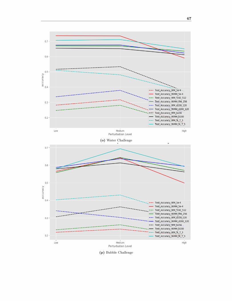
67
(o) Water Challenge
(p) Bubble Challenge