08 ant colony optimization 03 - webpages.iust.ac.ir

8. Ant Colony Optimization

8.3 The ACO Metaheuristic

Fall 2010

Instructor: Dr. Masoud Yaghini

Ant Colony Optimization: Part 3

Outline

Problem Representation

Ants’ Behavior

The Metaheuristic

The Traveling Salesman Problem

The Generalized Assignment Problem

The Multiple Knapsack Problem

References



An artificial ant in ACO is a stochastic constructive

procedure that incrementally builds a solution by

adding opportunely defined solution components to

a partial solution under construction.

The ACO metaheuristic can be applied to any The ACO metaheuristic can be applied to any

combinatorial optimization problems

The real issue is how to map the considered

problem to a representation that can be used by the

artificial ants to build solutions.



(S, f, Ω) The minimization problem

S The set of candidate solutions

f The objective function (cost)

Ω The set of constraints

f(s, t) An objective function (cost) value to each candidate

solution Ss∈ , and Ω(t) is a set of constraints at time t.

s Index for candidate solution, Ss∈

s* A globally optimal feasible solution, that is, a minimum

cost feasible solution to the minimization problem.

C A set of components, where C=c1, c2, …, cNc, and Nc

is the number of components.



x The state of the problem is defined in terms of

sequences of elements of C, x = <ci, cj, …, ch , …>

|x| The length of a sequence x, that is, the number of

components in the sequence

X The set of all possible states

~ ~X~

A set of feasible states, with XX ⊆~

S~

The set of feasible candidate solutions, with SS ⊆~

,

obtained from S via the constraints Ω(t).

S* A set of optimal solutions, with XS~*

⊆ and SS ⊆*

.

g(s, t) A cost is associated with each candidate solution

Ss∈ , In most cases g(s, t) = f(s, t)



GC =(C, L) The construction graph, which is completely

connected graph, whose nodes are the components C,

and the connections L fully connects the components

C.

ci The component of i, with Cci ∈

lij Ll ∈lij The connection of i and j, with Llij ∈

τ A pheromone trail, τi if associated with components, τij

if associated with connections

η A heuristic value, ηi if associated with components, ηij if

associated with connections.

In many cases η is the cost, or an estimate of the cost, of

adding the component or connection to the solution

under construction.


Implementing the constraints

• The problem constraints Ω(t) are implemented in the

policy followed by the artificial ants, as explained in

the next section.

• Implementing the constraints:

−− In a hard way, the ants can build only feasible

solutions

− In a soft way, the ants can build infeasible solutions

that can be penalized as a function of their degree of

infeasibility.


The Pheromone Trail

• The pheromone trail store in a long-term memory

about the entire ant search process, and is updated by

the ants themselves.

Ants’ Behavior


Ants’ Behavior

• Each ant exploits the construction graph GC =(C, L) to

search for optimal solutions ** Ss ∈ .

• Each ant has a memory Mk that it can use to store

information about the path it followed so far.

• Memory can be used to: • Memory can be used to:

1. Build feasible solutions (i.e., implement constraints

Ω)

2. Compute the heuristic values η

3. Evaluate the solution found

4. Retrace the path backward


Ants’ Behavior

• Each ant has a start state k

sx and one or more

termination conditions ek.

• Usually, the start state is expressed either as an empty

sequence or a single component.


Ants’ Behavior

• When in state xr = < xr-1, i>, if no termination condition

is satisfied, it moves to a node j in its neighborhood Nk

(xr), that is, to a state < xr-1, i> X∈ .

• If at least one of the termination conditions ek is

satisfied, then the ant stops. satisfied, then the ant stops.

• When an ant builds a candidate solution, moves to

infeasible states are forbidden in most applications


Ants’ Behavior

• Each ant selects a move by applying a probabilistic

decision rule.

• The probabilistic decision rule is a function of:

− the locally available pheromone trails and heuristic

values

− the problem constraints.


Ants’ Behavior

• When adding a component cj to the current state, it can

update the pheromone trail τ associated with it or with

the corresponding connection.

• Once it has built a solution, it can retrace the same path • Once it has built a solution, it can retrace the same path

backward and update the pheromone trails of the used

components.

The Metaheuristic


The ACO metaheuristic in pseudo-code


The Metaheuristic

Three procedures of an ACO :

– ConstructAntsSolutions

– UpdatePheromones

– DaemonActions


ConstructAntsSolutions


– manages a colony of ants that visit adjacent states of the

considered problem by moving through neighbor nodes

of the problem’s construction graph GC.

– They move by applying a stochastic local decision policy They move by applying a stochastic local decision policy

that makes use of pheromone trails and heuristic

information.

– Ants incrementally build solutions to the optimization

problem.




– Once an ant has built a solution, or while the solution is

being built, the ant evaluates the (partial) solution that

will be used by the UpdatePheromones procedure to

decide how much pheromone to deposit.


UpdatePheromones

UpdatePheromones

– is the process by which the pheromone trails are

modified.

– The pheromone value can:

Increase, as ants deposit pheromone on the components or Increase, as ants deposit pheromone on the components or

connections they use, or

Decrease, due to pheromone evaporation.

– The deposit of new pheromone increases the probability

that a good solution will be used again by future ants.


UpdatePheromones

UpdatePheromones

– Pheromone avoids a too rapid convergence of the

algorithm toward a suboptimal region, therefore favoring

the exploration of new areas of the search space.


DaemonActions

DaemonActions procedure

– is used to implement centralized actions which cannot be

performed by single ants.

– Examples of daemon actions are:

the activation of a local optimization procedure, or the activation of a local optimization procedure, or

the collection of global information

– that can be used to decide whether it is useful or not to

deposit additional pheromone to bias the search process

from a non-local perspective.


DaemonActions

DaemonActions procedure

– As a practical example, the daemon can observe the path

found by each ant in the colony and select one or a few

ants

– e.g., those that built the best solutions in the algorithm e.g., those that built the best solutions in the algorithm

iteration

– which are then allowed to deposit additional pheromone

on the components/connections they used.

The Traveling Salesman Problem


Traveling Salesman Problem

• The traveling salesman problem is the problem faced

by:

− a salesman who, starting from his home town,

− wants to find a shortest possible trip through a given

set of customer cities,

− visiting each city once

− finally returning home.



• The TSP can be represented by a complete weighted

graph G =(N, A) with:

− N : the set of n = |N| nodes (cities)

− A : the set of arcs fully connecting the nodes.

• Each arc Aji ∈),( is assigned a weight d which • Each arc Aji ∈),( is assigned a weight dij which

represents the distance between cities i and j.

• The TSP is the problem of finding a minimum length

Hamiltonian circuit of the graph, where a

Hamiltonian circuit is a closed walk (a tour) visiting

each node of G exactly once.



A solution to an instance of the TSP can be

represented as a permutation of the city indices

This permutation is cyclic, that is, the absolute

position of a city in a tour is not important at all but

only the relative order is important only the relative order is important


Construction Graph

• The construction graph GC =(C, L), where the set L

fully connects the components C, is identical to the

problem graph, that is C = N and L = A

• Each connection has a weight which corresponds to the

distance d between nodes i and j. distance dij between nodes i and j.

• The states of the problem are the set of all possible

tours.


Constraints

• The only constraint in the TSP is that all cities have to

be visited and that each city is visited at most once.

• This constraint is enforced if an ant at each

construction step chooses the next city only among

those it has not visited yet

• The feasible neighborhood k

iN of an ant k in city i,

where k is the ant’s identifier, comprises all cities that

are still unvisited.


Pheromone trails and heuristic information

• The pheromone trails are associated with arcs and

therefore τij in the TSP refer to the desirability of

visiting city j directly after i.

• The heuristic information ηij is typically inversely

proportional to the distance between cities i and j, a proportional to the distance between cities i and j, a

straightforward choice being ηij =1/dij.

• In fact, this is also the heuristic information used in

most ACO algorithms for the TSP.


Solution construction

Each ant is initially put on a randomly chosen start

city and at each step iteratively adds one still

unvisited city to its partial tour.

The solution construction terminates once all cities

have been visited.have been visited.


Dynamic Traveling Salesman Problem

The dynamic traveling salesman problem

(DTSP) is a TSP in which cities can be added or

removed at run time.

The goal is to find as quickly as possible the new

shortest tour after each transition.shortest tour after each transition.


Dynamic Traveling Salesman Problem

Construction graph

– The same as for the TSP: GC(C, L)，where C(t) is the set

of cities and L = L(t) completely connects GC.

– The dependence of C and L on time is due to the dynamic

nature of the problem.nature of the problem.



In the generalized assignment problem (GAP) a

set of tasks i œ I , has to be assigned to a set of

agents j œ J.

Each agent j has only a limited capacity aj and each

task i assigned to agent j consumes a quantity rij of task i assigned to agent j consumes a quantity rij of

the agent’s capacity.

Also, the cost dij of assigning task i to agent j is

given.

The objective then is to find a feasible task

assignment with minimum cost.



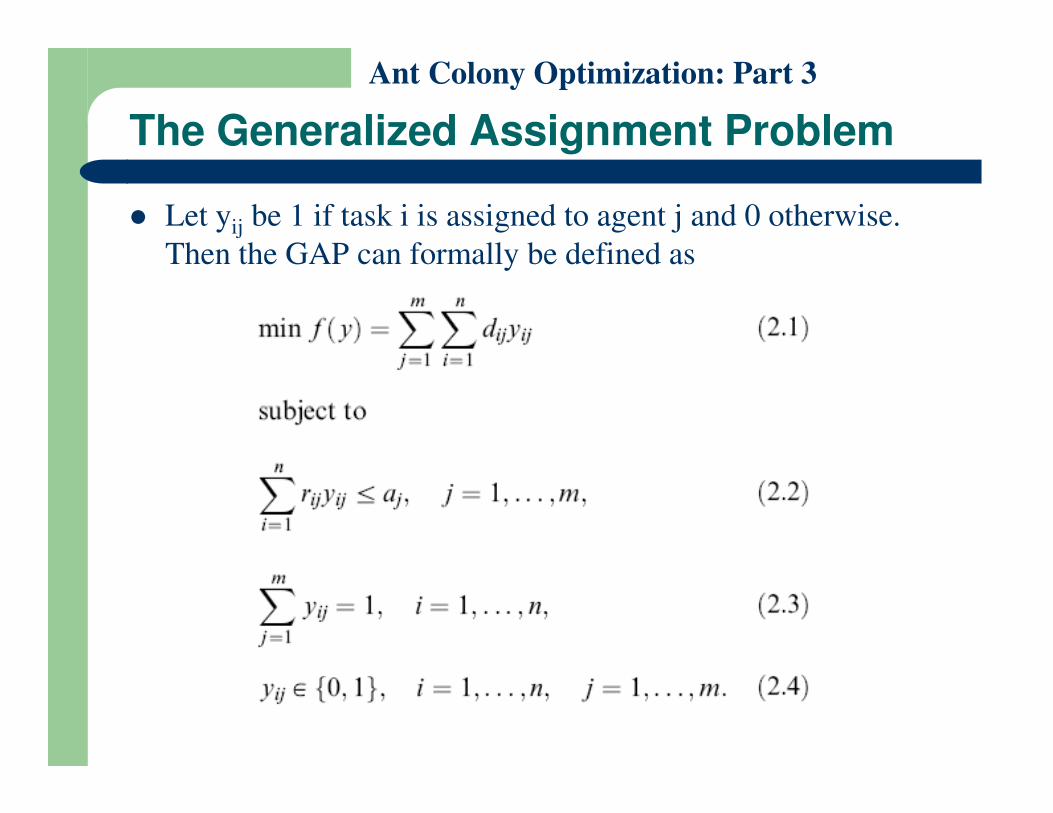
Let yij be 1 if task i is assigned to agent j and 0 otherwise.

Then the GAP can formally be defined as



The constraints in equation (2.2) implement the

limited resource capacity of the agents,

The constraints given by equations (2.3) and (2.4)

impose that each task is assigned to exactly one

agent and that a task cannot be split among several agent and that a task cannot be split among several

agents.


Construction graph

The problem could be represented on the

construction graph GC = (C, L) in which the set of

components comprises the set of tasks and agents,

that is, C = I » J.

Each assignment, which consists of n couplings (i, Each assignment, which consists of n couplings (i,

j) of tasks and agents, corresponds to at least one

ant’s walk on this graph and costs dij are associated

with all possible couplings (i, j) of tasks and agents.


Constraints

Walks on the construction graph GC have to satisfy

the constraints given by equations (2.3) and (2.4) to

obtain a valid assignment.

One particular way of generating such an

assignment is by an ant’s walk which iteratively assignment is by an ant’s walk which iteratively

switches from task nodes (nodes in the set I) to

agent nodes (nodes in the set J) without repeating

any task node but possibly using an agent node

several times (several tasks may be assigned to an

agent).


Constraints

Moreover, the GAP involves resource capacity

constraints that can be enforced by an appropriately

defined neighborhood.

For example, for an ant k, Nik could be defined as

consisting of all those agents to which task i can be consisting of all those agents to which task i can be

assigned without violating the agents’ resource

capacity.


Constraints

If no agent meets the task’s resource requirement,

then the ant is forced to build an infeasible solution

– In this case Nik becomes the set of all agents.

Infeasibilities can then be handled,

– for example, by assigning penalties proportional to the – for example, by assigning penalties proportional to the

amount of resource violations.



During the construction of a solution, ants

repeatedly have to take the following two basic

decisions:

– (1) choose the task to assign next

– (2) choose the agent the task should be assigned to. – (2) choose the agent the task should be assigned to.



Pheromone trail information can be associated with

any of the two decisions

– it can be used to learn an appropriate order for task

assignments, τij represents the desirability of assigning

task j directly after task i

– it can be associated with the desirability of assigning a

task to a specific agent, τij represents the desirability of

assigning agent j to task i.



Similarly, heuristic information can be associated

with any of the two decisions.

– For example, heuristic information could bias task

assignment toward those tasks that use more resources,

and

– Bias the choice of agents in such a way that small

assignment costs are incurred and the agent only needs a

relatively small amount of its available resource to

perform the task.




– can be performed as usual, by choosing the components

to add to the partial solution from among those that, as

explained above,

– satisfy the constraints with a probability biased by the satisfy the constraints with a probability biased by the

pheromone trails and heuristic information.



Given a set of items i œ I with associated a vector of

resource requirements ri and a profit bi

The knapsack problem (KP) is the problem of

selecting a subset of items from I in such a way that

they fit into a knapsack of limited capacity and they fit into a knapsack of limited capacity and

maximize the sum of profits of the chosen items.

The multiple knapsack problem (MKP), also

known as multidimensional KP, extends the single

KP by considering multiple resource constraints.



Let yi be a variable associated with item i, which has

value 1 if i is added to the knapsack, and 0

otherwise.

Also, let rij be the resource requirement of item i

with respect to resource constraint j, aj the capacity with respect to resource constraint j, aj the capacity

of resource j, and m be the number of resource

constraints.

In the MKP, it is typically assumed that all profits bi

and all weights rij take positive values.



The MKP can be formulated as


Construction graph

In the construction graph GC = (C, L), the set of

components C corresponds to the set of items and,

as usual, the set of connections L fully connects the

set of items.

The profit of adding items can be associated with The profit of adding items can be associated with

either the connections or the components.


Constraints

The solution construction has to consider the

resource constraints given by equation (2.6).

During the solution construction process, this can be

easily done by allowing ants to add only those

components that, when added to their current partial components that, when added to their current partial

solution, do not violate any resource constraint.



The MKP has the particularity that pheromone trails

τij are associated only with components and refer to

the desirability of adding an item i to the current

partial solution.

The heuristic information, intuitively, should prefer The heuristic information, intuitively, should prefer

items which have a high profit and low resource

requirements.



One possible choice for the heuristic information is

to calculate the average resource requirement :

for each item and then to define: for each item and then to define:

Yet this choice has the disadvantage that it does not

take into account how tight the single resource

constraints are.



Therefore, more information can be provided if the

heuristic information is also made a function of the

aj.

One such possibility is to calculate:

and to compute the heuristic information as:



Each ant iteratively adds items in a probabilistic

way biased by pheromone trails and heuristic

information

Each item can be added at most once.

An ant’s solution construction ends if no item can An ant’s solution construction ends if no item can

be added anymore without violating any of the

resource constraints.

This leads to one particularity of the ACO

application to the MKP

References


References

M. Dorigo and T. Stützle. Ant Colony

Optimization, MIT Press, Cambridge, 2004.

The End

08 ant colony optimization 03 - webpages.iust.ac.ir

Documents