05-wcdma rf optimization
TRANSCRIPT

Huawei Confidential. All Rights Reserved
WCDMA RF Optimization
ISSUE 1.0

Internal Use 2
This lecture introduces the various stages involved in optimizing a 3G radio network and focuses mainly on the RF Optimization phase.
Step-by-step approach for the analysis of drive survey data collected by Agilent Scanner and test UE is presented. The analysis is carried out using the post processing tool “Actix Analyzer”.
Internal Use 3
RF optimization will be an ongoing activity and will need to be revisited as traffic increases in the network and as new sites are deployed.
In addition, as the network matures, the optimization process should be enhanced to take into account statistical data and key performance indicators collected throughout the network.

Internal Use 4
Chapter 1 Chapter 1 Optimization PhasesOptimization Phases
Chapter 2 RF Optimization
Chapter 3 RF Analysis Approaches
Chapter 4 Antenna Adjustment Example
Chapter 5 Drop Call Analysis Example

Internal Use 5
Network Optimization Phases – Flow ChartNetwork Optimization Phases – Flow Chart
New Site Integrated
Single Site Verification
RF Optimization
Cluster of Sites Ready?
Service Test and Parameter Optimization
Regular Reference Route Testing and Stats Analysis
Re-optimization Needed?
Y
N
N
Y

Internal Use 6
Network Optimization Phases – Step 1Network Optimization Phases – Step 1
Single Site Verification To verify the functionality of every new site.
Objectives To ensure there are no faults related to site installation or
parameter settings.

Internal Use 7
Network Optimization Phases – Step 2Network Optimization Phases – Step 2
RF Optimization Once all the sites in a given area are integrated and
verified, RF (or Cluster) optimization could begin. Objectives
To optimize coverage while in the same time keeping interference and pilot pollution under control over the target area. This phase also includes the verification and optimization of the 3G neighbor lists.
Internal Use 8
Network Optimization Phases – Step 3Network Optimization Phases – Step 3
Services Testing & Parameter Optimization To be conducted in areas of good RF conditions in order
to exclude any coverage issues. Such testing does not need to be performed for each cell but the drive route must include different clutter types and environments.
Objectives To assess the performance and identify any need for
specific parameter optimization.
Internal Use 9
Network Optimization Phases – Step 4Network Optimization Phases – Step 4
Regular Reference Route Testing & Stats Analysis Constant monitoring and evaluation of the network
performance can be based on field testing as well as network stats analysis.
Results of the regular analysis may necessitate re-visits to the RF optimization and/or parameters’ tuning.
Objectives To identify any new issues that could arise, for example,
as a result of increase in traffic or changes in the environment.
Internal Use 10
Chapter 1 Optimization Phases
Chapter 2Chapter 2 RF OptimizationRF Optimization
Chapter 3 RF Analysis Approaches
Chapter 4 Antenna Adjustment Example
Chapter 5 Drop Call Analysis Example
Internal Use 11
RF Optimization - PreparationRF Optimization - Preparation
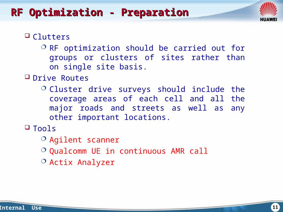
Clutters RF optimization should be carried out for groups or
clusters of sites rather than on single site basis. Drive Routes
Cluster drive surveys should include the coverage areas of each cell and all the major roads and streets as well as any other important locations.
Tools Agilent scanner Qualcomm UE in continuous AMR call Actix Analyzer
Internal Use 12
RF Optimization - RF Optimization - TargetsTargets
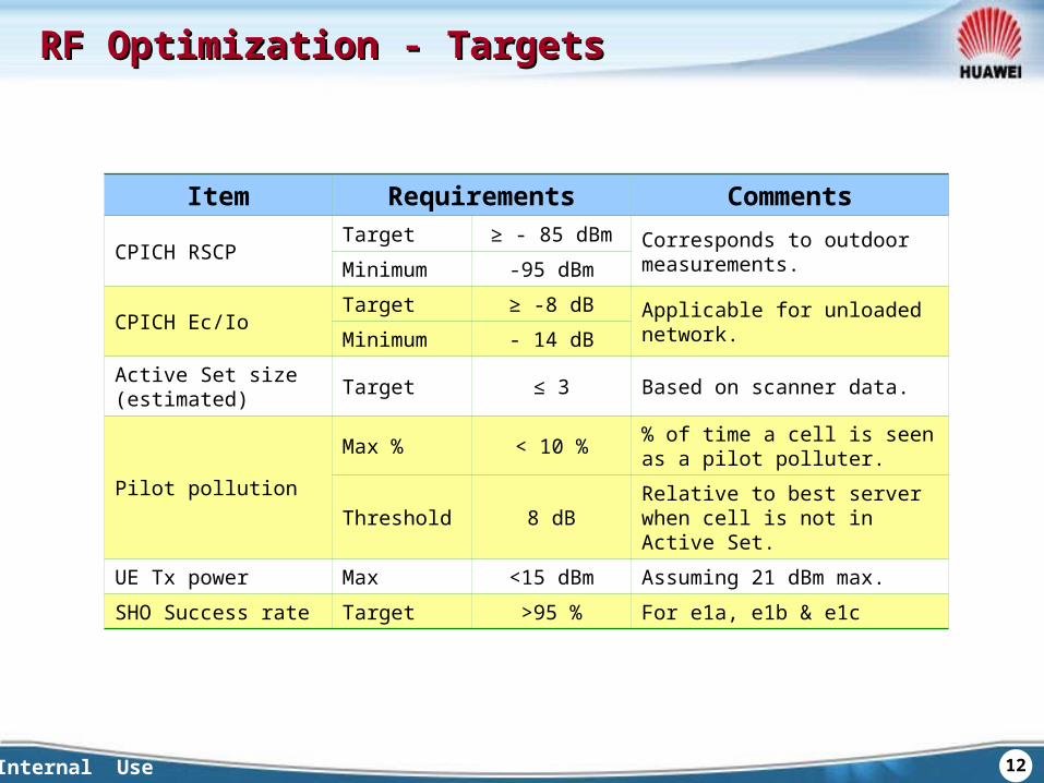
Item Requirements Comments
CPICH RSCPTarget ≥ - 85 dBm Corresponds to outdoor
measurements.Minimum -95 dBm
CPICH Ec/IoTarget ≥ -8 dB
Applicable for unloaded network.Minimum - 14 dB
Active Set size (estimated)
Target ≤ 3 Based on scanner data.
Pilot pollution
Max % < 10 %% of time a cell is seen as a pilot polluter.
Threshold 8 dBRelative to best server when cell is not in Active Set.
UE Tx power Max <15 dBm Assuming 21 dBm max.
SHO Success rate Target >95 % For e1a, e1b & e1c
Internal Use 13
RF Optimization – Flow ChartRF Optimization – Flow Chart
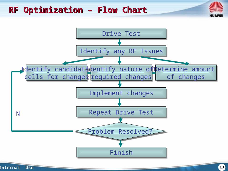
Drive TestDrive Test
Identify any RF IssuesIdentify any RF Issues
Identify candidate cells for changes
Identify candidate cells for changes
Identify nature of required changes
Identify nature of required changes
Determine amount of changes
Determine amount of changes
Implement changesImplement changes
Repeat Drive TestRepeat Drive Test
FinishFinish
N
Problem Resolved?Problem Resolved?
Internal Use 14
RF Optimization - SolutionsRF Optimization - Solutions
Antenna tilt
Antenna azimuth
Antenna location
Antenna height
Antenna type
Site location
New site
Internal Use 15
Chapter 1 Optimization Phases
Chapter 2 RF Optimization
Chapter 3Chapter 3 RF Analysis ApproachesRF Analysis Approaches
Chapter 4 Antenna Adjustment Example
Chapter 5 Drop Call Analysis Example
Internal Use 16
RF Analysis Approaches – Cell DominanceRF Analysis Approaches – Cell Dominance
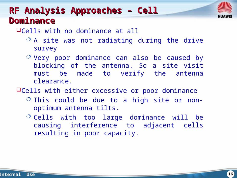
Cells with no dominance at all A site was not radiating during the drive survey Very poor dominance can also be caused by blocking of
the antenna. So a site visit must be made to verify the antenna clearance.
Cells with either excessive or poor dominance This could be due to a high site or non-optimum antenna
tilts. Cells with too large dominance will be causing
interference to adjacent cells resulting in poor capacity.
Internal Use 17
RF Analysis Approaches – Cell DominanceRF Analysis Approaches – Cell Dominance
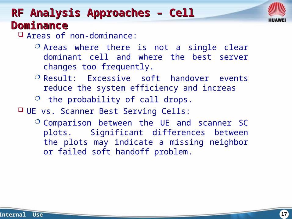
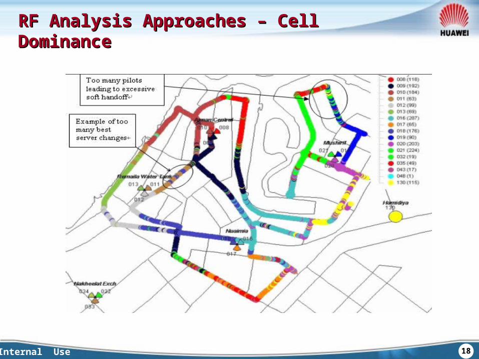
Areas of non-dominance: Areas where there is not a single clear dominant cell and
where the best server changes too frequently. Result: Excessive soft handover events reduce the
system efficiency and increas the probability of call drops.
UE vs. Scanner Best Serving Cells: Comparison between the UE and scanner SC plots.
Significant differences between the plots may indicate a missing neighbor or failed soft handoff problem.
Internal Use 18
RF Analysis Approaches – Cell DominanceRF Analysis Approaches – Cell Dominance
Internal Use 19
RF Analysis Approaches – RF Analysis Approaches – CPICH Coverage CPICH Coverage
Check areas of poor coverage, suggestion value as below: Good: RSCP ≥ -85 dBm Fair: -95 dBm ≤ RSCP < -85 dBm Poor: RSCP < - 95 dBm
Examine the RSCP coverage on per cell bases in order to highlight any cells that have too large a footprint.

Internal Use 20
RF Analysis Approaches – RF Analysis Approaches – CPICH CoverageCPICH Coverage
Internal Use 21
RF Analysis Approaches – RF Analysis Approaches – InterferenceInterference
CPICH Ec/Io Plot Good: Ec/Io ≥ -8 dB Fair: -14 dB ≤ Ec/Io < -8 dB Poor: Ec/Io < - 14 dB
The -8 dB threshold takes into account the expected future interference increase as a result of increased traffic.

Internal Use 22
RF Analysis Approaches – RF Analysis Approaches – InterferenceInterference
Because the RSCP Level is poor, and the fundamental cause of low Ec/Io is poor coverage
Because the RSCP Level is poor, and the fundamental cause of low Ec/Io is poor coverage
-15.5
-104
-20
-19
-18
-17
-16
-15
-14
Ec/Io RSCP-120
-115
-110
-105
-100
-95
-90
What’s the problem?

Internal Use 23
RF Analysis Approaches – RF Analysis Approaches – InterferenceInterference
RSCP level is good, and this will imply strong system interference
RSCP level is good, and this will imply strong system interference
-15.5
-63
-20
-19
-18
-17
-16
-15
-14
Ec/Io RSCP-90
-85
-80
-75
-70
-65
-60 What’s the problem?

Internal Use 24
RF Analysis Approaches – RF Analysis Approaches – InterferenceInterference
Internal Use 25
RF Analysis Approaches – UL CoverageRF Analysis Approaches – UL Coverage
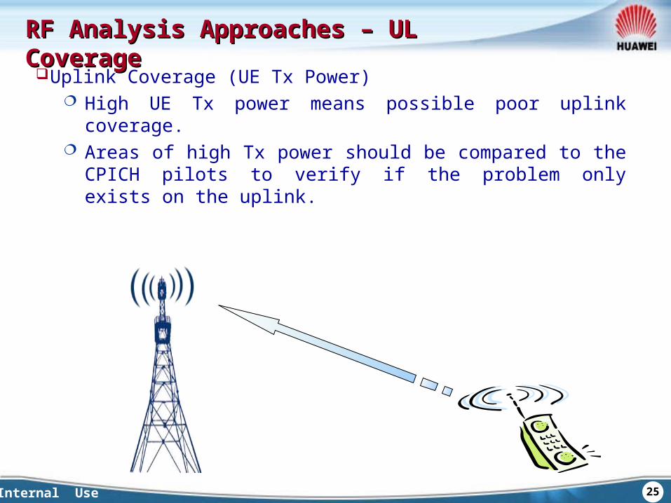
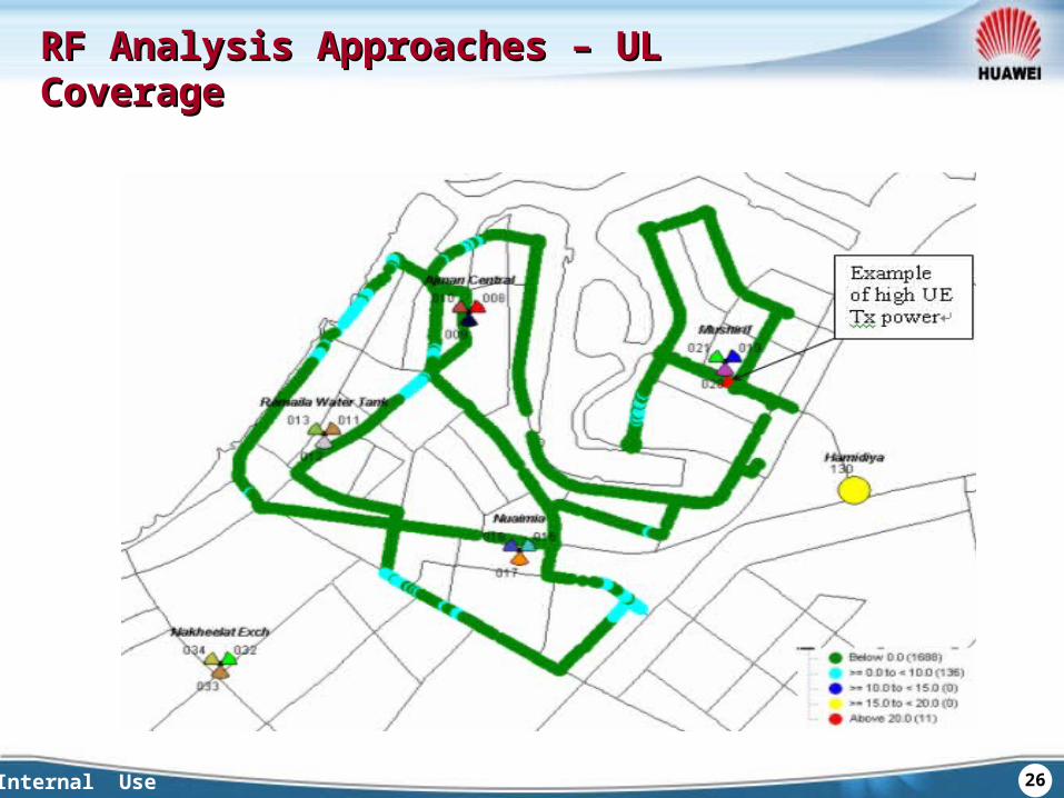
Uplink Coverage (UE Tx Power) High UE Tx power means possible poor uplink coverage. Areas of high Tx power should be compared to the CPICH pilots
to verify if the problem only exists on the uplink.
Internal Use 26
RF Analysis Approaches – UL CoverageRF Analysis Approaches – UL Coverage
Internal Use 27
RF Analysis Approaches – Pilot PollutionRF Analysis Approaches – Pilot Pollution
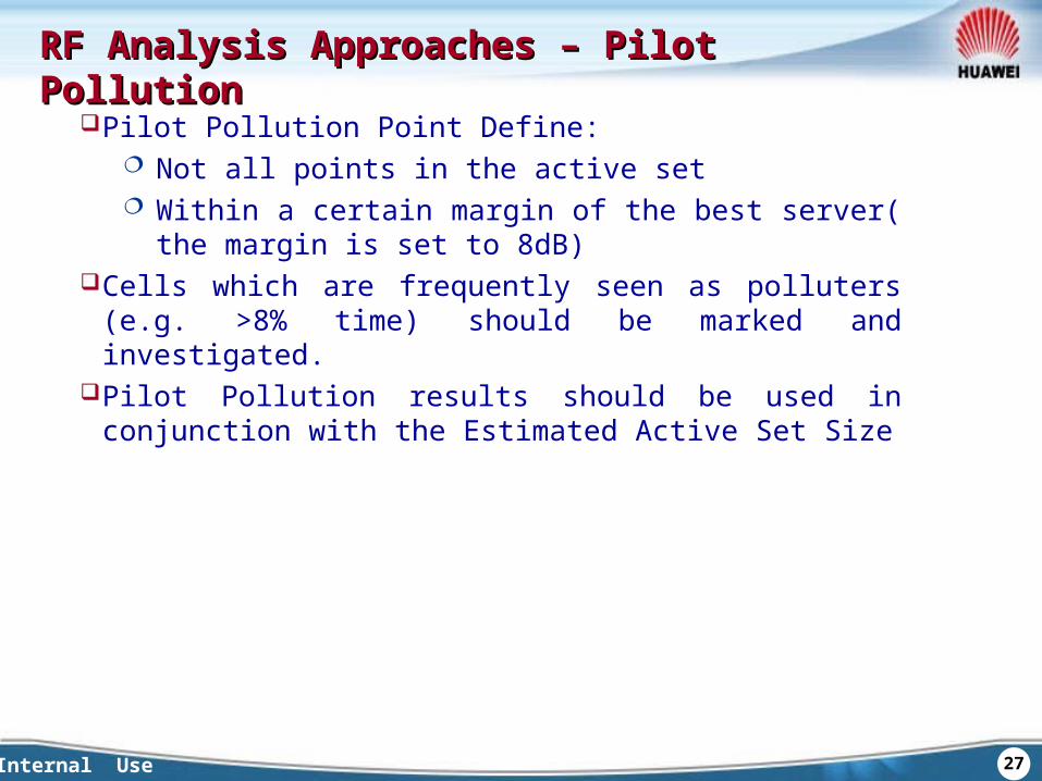
Pilot Pollution Point Define: Not all points in the active set Within a certain margin of the best server( the margin is
set to 8dB)Cells which are frequently seen as polluters (e.g. >8% time)
should be marked and investigated. Pilot Pollution results should be used in conjunction with the
Estimated Active Set Size

Internal Use 28
RF Analysis Approaches – Pilot PollutionRF Analysis Approaches – Pilot Pollution
-62 -64 -66 -68 -69
-81
-90
-85
-80
-75
-70
-65
-60
SC1 SC2 SC3 SC4 SC5 SC6
RSC
P (d
Bm)
Active Set Pilot Pollution
Margin
NotPilot Pollution
Internal Use 29
RF Analysis Approaches – Pilot PollutionRF Analysis Approaches – Pilot Pollution
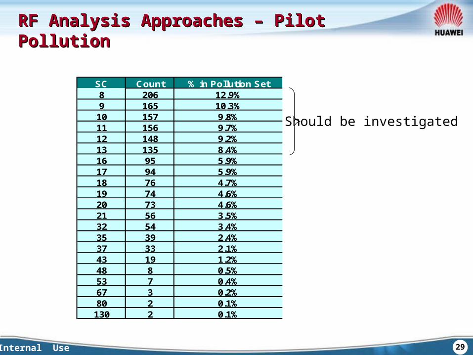
SC Count % in Pollution Set8 206 12.9%9 165 10.3%
10 157 9.8%11 156 9.7%12 148 9.2%13 135 8.4%16 95 5.9%17 94 5.9%18 76 4.7%19 74 4.6%20 73 4.6%21 56 3.5%32 54 3.4%35 39 2.4%37 33 2.1%43 19 1.2%48 8 0.5%53 7 0.4%67 3 0.2%80 2 0.1%
130 2 0.1%
Should be investigated

Internal Use 30
RF Analysis Approaches – Pilot PollutionRF Analysis Approaches – Pilot Pollution
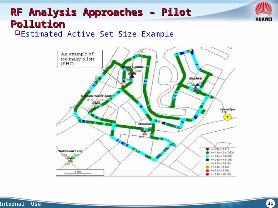
Estimated Active Set Size Another useful measure of pilot pollution is by looking at
the estimated active set based on the scanner data. This plot is obtained by modeling the network soft handoff parameters within Actix.
In order to see areas of excessive SHO candidates, the estimated active set size is allowed to exceed maximum of 3.
This can be done in conjunction with the Pilot pollution analysis.
Internal Use 31
RF Analysis Approaches – Pilot PollutionRF Analysis Approaches – Pilot Pollution
Estimated Active Set Size Example
Internal Use 32
RF Analysis Approaches – Neighbor ListRF Analysis Approaches – Neighbor List
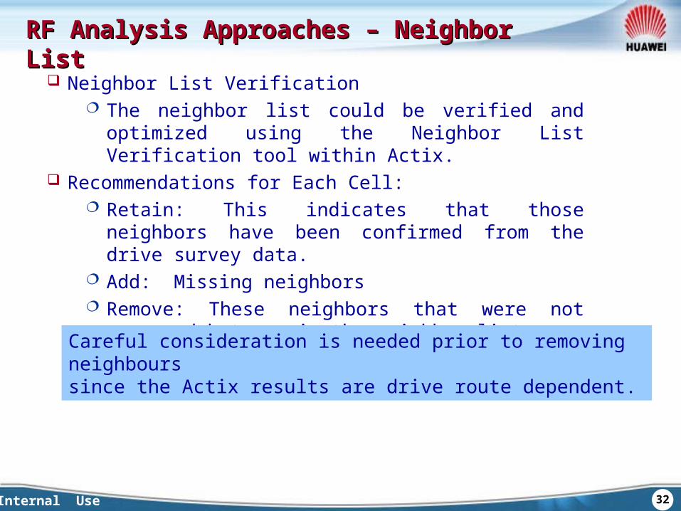
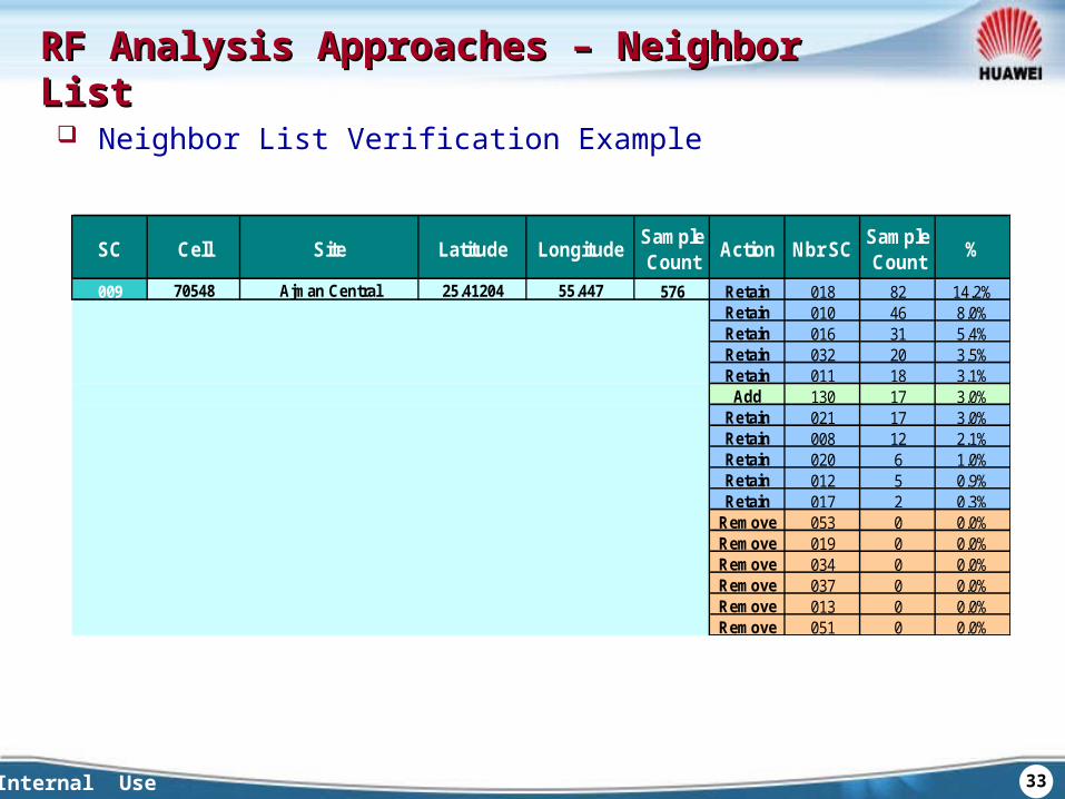
Neighbor List Verification The neighbor list could be verified and optimized using
the Neighbor List Verification tool within Actix. Recommendations for Each Cell:
Retain: This indicates that those neighbors have been confirmed from the drive survey data.
Add: Missing neighbors Remove: These neighbors that were not measured but
are in the neighbor list.
Careful consideration is needed prior to removing neighbours since the Actix results are drive route dependent.
Internal Use 33
RF Analysis Approaches – Neighbor ListRF Analysis Approaches – Neighbor List
Neighbor List Verification Example
009 576 Retain 018 82 14.2%Retain 010 46 8.0%Retain 016 31 5.4%Retain 032 20 3.5%Retain 011 18 3.1%
Add 130 17 3.0%Retain 021 17 3.0%Retain 008 12 2.1%Retain 020 6 1.0%Retain 012 5 0.9%Retain 017 2 0.3%
Remove 053 0 0.0%Remove 019 0 0.0%Remove 034 0 0.0%Remove 037 0 0.0%Remove 013 0 0.0%Remove 051 0 0.0%
70548 Ajman Central 25.41204 55.447
Nbr SCSample Count
%Latitude LongitudeSample Count
ActionSC Cell Site
Internal Use 34
RF Analysis Approaches – SHORF Analysis Approaches – SHO
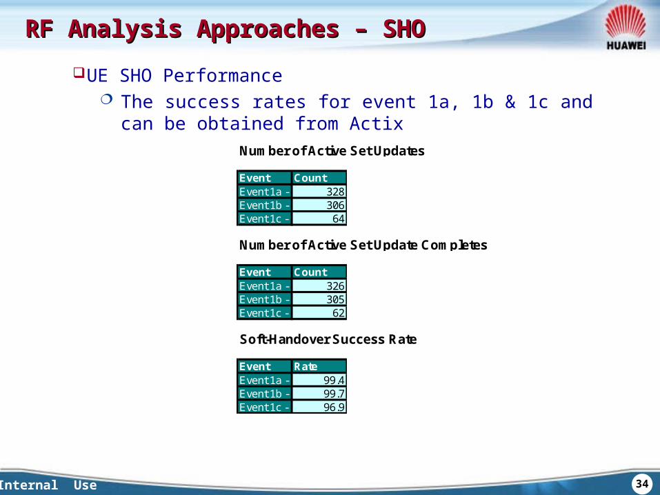
UE SHO Performance The success rates for event 1a, 1b & 1c and can be
obtained from Actix Number of Active Set Updates
Event CountEvent 1a - Cell Addition328Event 1b - Cell Removal306Event 1c - Cell Replacement64
Number of Active Set Update Completes
Event CountEvent 1a - Cell Addition326Event 1b - Cell Removal305Event 1c - Cell Replacement62
Soft-Handover Success Rate
Event RateEvent 1a - Cell Addition99.4Event 1b - Cell Removal99.7Event 1c - Cell Replacement96.9

Internal Use 35
RF Analysis Approaches – Call DropRF Analysis Approaches – Call Drop
Drop Call Analysis - RF related issues : Poor coverage (RSCP & Ec/Io) High interference and hence poor Ec/Io Poor uplink coverage (insufficient UE Tx power) Poor dominance (best cell changes too frequently
resulting in too many SHO events) Pilot pollution (too many cells present) Missing neighbors Fast change of RF conditions (e.g. turning a corner)
Internal Use 36
RF Analysis Approaches – Call DropRF Analysis Approaches – Call Drop
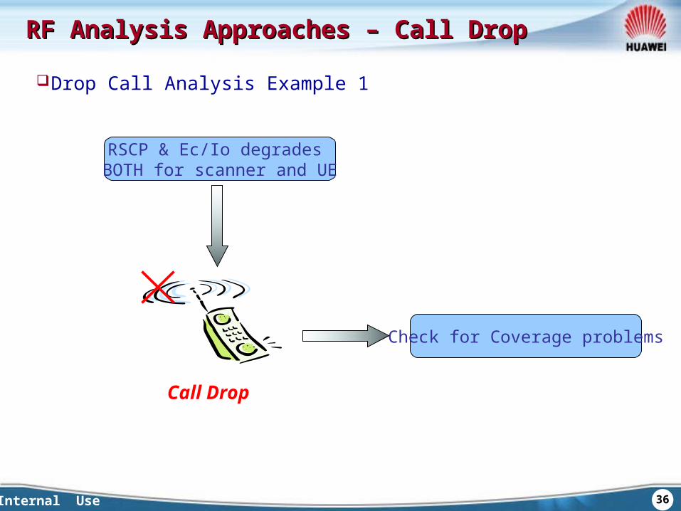
Drop Call Analysis Example 1
Call Drop
RSCP & Ec/Io degrades BOTH for scanner and UE
Check for Coverage problems

Internal Use 37
RF Analysis Approaches – Call DropRF Analysis Approaches – Call Drop
Drop Call Analysis Example 2
Call Drop
Ec/Io (and RSCP) degrades for UE ONLY while scanner shows no degradation
Ec/Io (and RSCP) degrades for UE ONLY while scanner shows no degradation
UE camp on new cell immediately after drop, and UE did not
measure this cell before Drop
UE camp on new cell immediately after drop, and UE did not
measure this cell before Drop
Check the NeighborCheck the Neighbor

Internal Use 38
RF Analysis Approaches – Call DropRF Analysis Approaches – Call Drop
Drop Call Analysis Example 3
Call Drop
Too many and too quick changes of best server
Too many and too quick changes of best server
UE to perform measurements and SHO in time difficultly
UE to perform measurements and SHO in time difficultly
Ping-Pong Handover, need to improve cell dominance
Ping-Pong Handover, need to improve cell dominance

Internal Use 39
Chapter 1 Optimization Phases
Chapter 2 RF Optimization
Chapter 3 RF Analysis Approaches
Chapter 4Chapter 4 Antenna Adjustment ExampleAntenna Adjustment Example
Chapter 5 Drop Call Analysis Example

Internal Use 40
Antenna Adjustment ExampleAntenna Adjustment Example
RSCP Coverage before Adjustment

Internal Use 41
Antenna Adjustment ExampleAntenna Adjustment Example
RSCP Coverage after Adjustment
Internal Use 42
Antenna Adjustment ExampleAntenna Adjustment Example
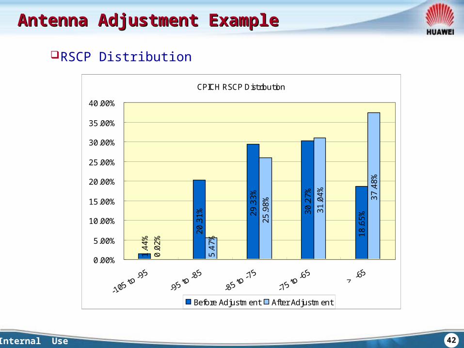
RSCP Distribution
CPICH RSCP Distribution
1.44
%
20.3
1% 29.3
3%
30.2
7%
18.6
5%
0.02
%
5.47
%
25.9
8%
31.0
4% 37.4
8%
0.00%
5.00%
10.00%
15.00%
20.00%
25.00%
30.00%
35.00%
40.00%
Before Adjustment After Adjustment

Internal Use 43
Antenna Adjustment ExampleAntenna Adjustment Example
Down Tilt from 4 to 6 Result
Internal Use 44
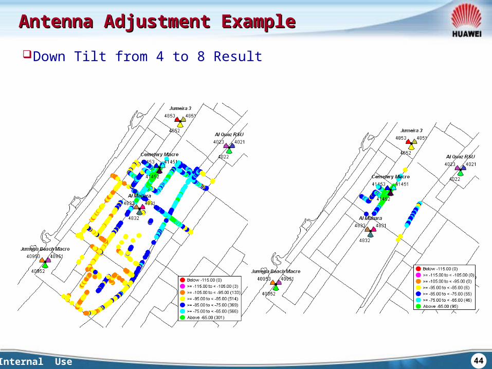
Antenna Adjustment ExampleAntenna Adjustment Example
Down Tilt from 4 to 8 Result
Internal Use 45
Chapter 1 Optimization Phases
Chapter 2 RF Optimization
Chapter 3 RF Analysis Approaches
Chapter 4 Antenna Adjustment Example
Chapter 5Chapter 5 Drop Call Analysis ExampleDrop Call Analysis Example
Internal Use 46
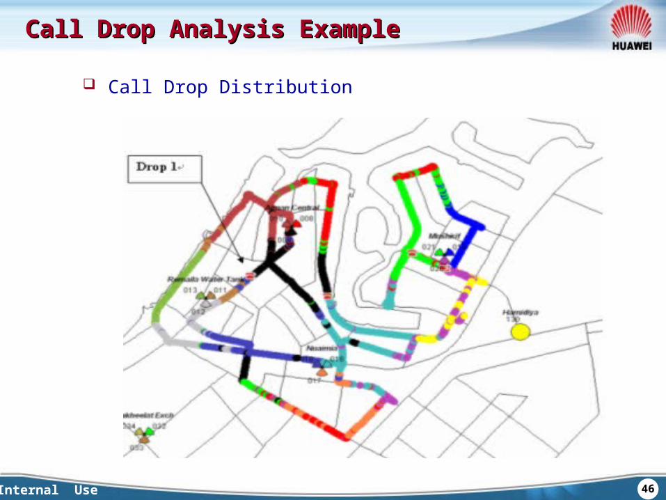
Call Drop Analysis ExampleCall Drop Analysis Example
Call Drop Distribution
Internal Use 47
Call Drop Analysis ExampleCall Drop Analysis Example
There are total 5 drop calls in the plot.
The example of drop call 1 is analyzed to show the process of analysis in the following.
Call drop 1 occurred at an area of frequent change of best server as shown by the scanner scrambling code plot
Internal Use 48
Call Drop Analysis ExampleCall Drop Analysis Example
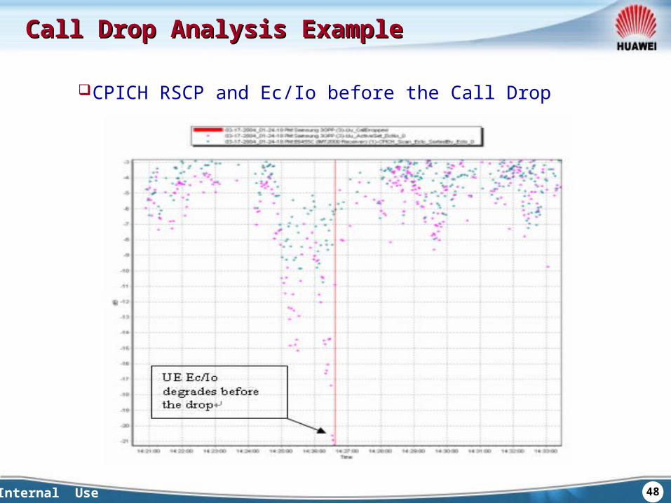
CPICH RSCP and Ec/Io before the Call Drop

Internal Use 49
Call Drop Analysis ExampleCall Drop Analysis Example
Compare Ec/Io from both scanner and UE at the time of the drop as shown in Figure. This clearly shows the UE Ec/Io to drop to < -21 dB while the scanner remained above -11 dB.

Internal Use 50
Call Drop Analysis ExampleCall Drop Analysis Example
Best server before and after the Call Drop
Internal Use 51
Call Drop Analysis ExampleCall Drop Analysis Example
Comparing the best servers from the UE and the scanner at the time of drop:
Call Drop 1 (UE vs. scanner best server) shows that SC008 is the best server before call drop in both UE and scanner. However, about 30 seconds before the drop, the scanner selected SC018 as the best server while the UE continued to have only SC009 in its active set resulting in the drop call. Immediately after the drop, the UE camps on SC018.

Internal Use 52
Call Drop Analysis ExampleCall Drop Analysis Example
UE Active Set and Monitor Set Before and After the Call Drop
Internal Use 53
Call Drop Analysis ExampleCall Drop Analysis Example
Conclusion Examining the UE Active and Monitored set, Figure does not
show SC018 to be measured by the UE prior to the drop. This scenario resembles a missing neighbor problem
Internal Use 54
Call Drop Analysis ExampleCall Drop Analysis Example
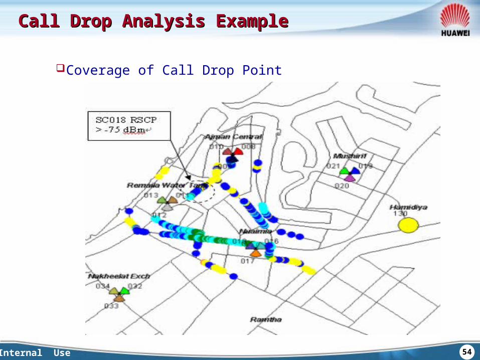
Coverage of Call Drop Point

Internal Use 55
Call Drop Analysis ExampleCall Drop Analysis Example
Solution: Looking at call drop Figure clearly shows that at the
location of the drop, SC018 should not be the best server.
Cell SC018 clearly requires some down tilting to control its interference into the area of Drop 1. To illustrate this, RSCP coverage of SC018 shows clearly that the cell’s is extending into a large area. E.g. around the location of drop call, SC018 RSCP is > -75dBm.
Add the Missing Neighbors

Huawei Confidential. All Rights Reserved