02 demand and supply analysis

8/3/2019 02 Demand and Supply Analysis

http://slidepdf.com/reader/full/02-demand-and-supply-analysis 1/33

1

1. Competitive Markets Defined

2. Market Demand

3. Market Supply

4. Market Equilibrium

5. Characterizing Demand and Supply: Elasticity



2

Definition: Competitive markets are those with sellersand buyers that are small and numerous enoughthat they take the market price as given whenthey decide how much to buy and sell.

as opposed to monopolies and oligopolies (see later)

A market is characterized along 3 dimensions:

• the commodity (what is traded on the market)

• the geography (where is the market)

• the time (when does the trade take place)

1. Competitive Markets



3

Definition: the market demand function tells us howthe total quantity of a good demanded dependson various factors:

Qd = Q(P, Po, I,…)

Definition: the market demand curve plots theaggregate quantity of a good that consumersare willing to buy at different prices, holding constant other demand drivers ( such as pricesof other goods, consumer income, quality,...)

Qd = Q(P)

2. Market Demand



4

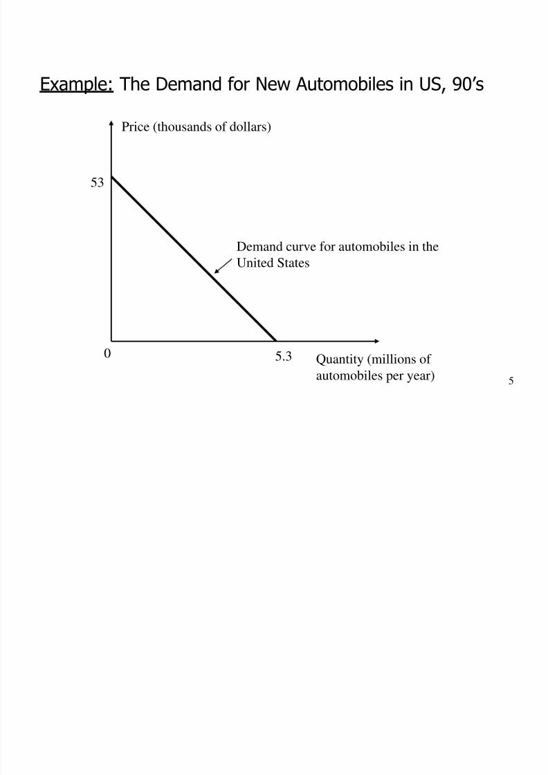
Example:Qd = 100 - 2P

Convention!

Economists always draw the quantity on the X-axis(endogenous variable) and the price on the Y-axis(exogenous variable)

Therefore, we often define the inverse demand curve:P = P(Qd)

P = 50 - Qd /2 (draw!)



5

0 Quantity (millions of

automobiles per year)

Price (thousands of dollars)

Demand curve for automobiles in the

United States

53

5.3

Example: The Demand for New Automobiles in US, 90’s



6

Definition: The law of demand is the empirical regularitythat, all other things being equal , thequantity of a good demanded decreases when

the price of this good increases.

the demand curve is always downward sloping

The Law of Demand



7

Movement along the demand curve means a change in theown price of the good.

If any other factor that affects the demand changes, thedemand curve shifts … • If the change increases the willingness of consumers to acquire the

good, the demand curve shifts to the right (outward shift)• If the change decreases the willingness of consumers to acquire the

good, the demand curve shifts to the left (inward shift)

Demand curve cte.P

Q

Qd1 Qd

2

P

QQd



8

Definition: the market supply function tells us howthe quantity of a good supplied by the sum of all producers in the market depends on variousfactors:

Qs = Q(P, Po, W,…)

Definition: the market supply curve plots the aggregatequantity of a good that will be offered for sale

at different prices, holding constant other supply drivers

Qs = Q(P)

3. Market Supply



9

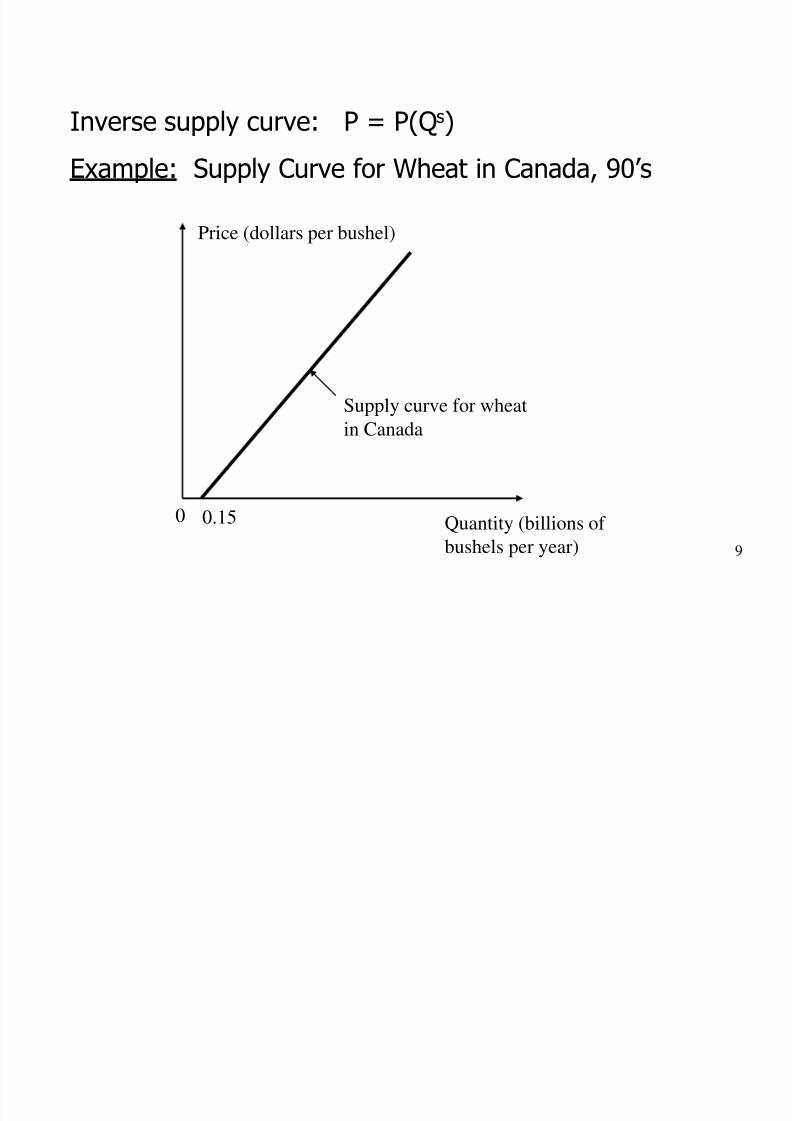
Inverse supply curve: P = P(Qs)

Example: Supply Curve for Wheat in Canada, 90’s

0 Quantity (billions of

bushels per year)

Price (dollars per bushel)

Supply curve for wheatin Canada

0.15



10

Definition: The law of supply is the empirical regularitythat, all other things being equal, the quantityof a good offered increases when the price of

this good increases.

the supply curve is always upward sloping

The Law of Supply



11

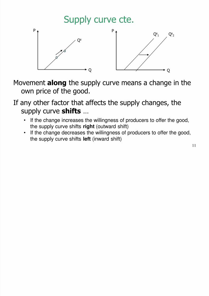
Movement along the supply curve means a change in theown price of the good.

If any other factor that affects the supply changes, the

supply curve shifts … • If the change increases the willingness of producers to offer the good,

the supply curve shifts right (outward shift)

• If the change decreases the willingness of producers to offer the good,

the supply curve shifts left (inward shift)

Supply curve cte.P

Q

Qs

P

Q

Qs

1

Qs

2



12

Definition: A market equilibrium is a price such that, atthis price, the quantities demanded andsupplied are the same.

(Demand and supply curves intersect at equilibrium)

4. Market Equilibrium

P

Q

Qs

Qd

P*

Q*



13

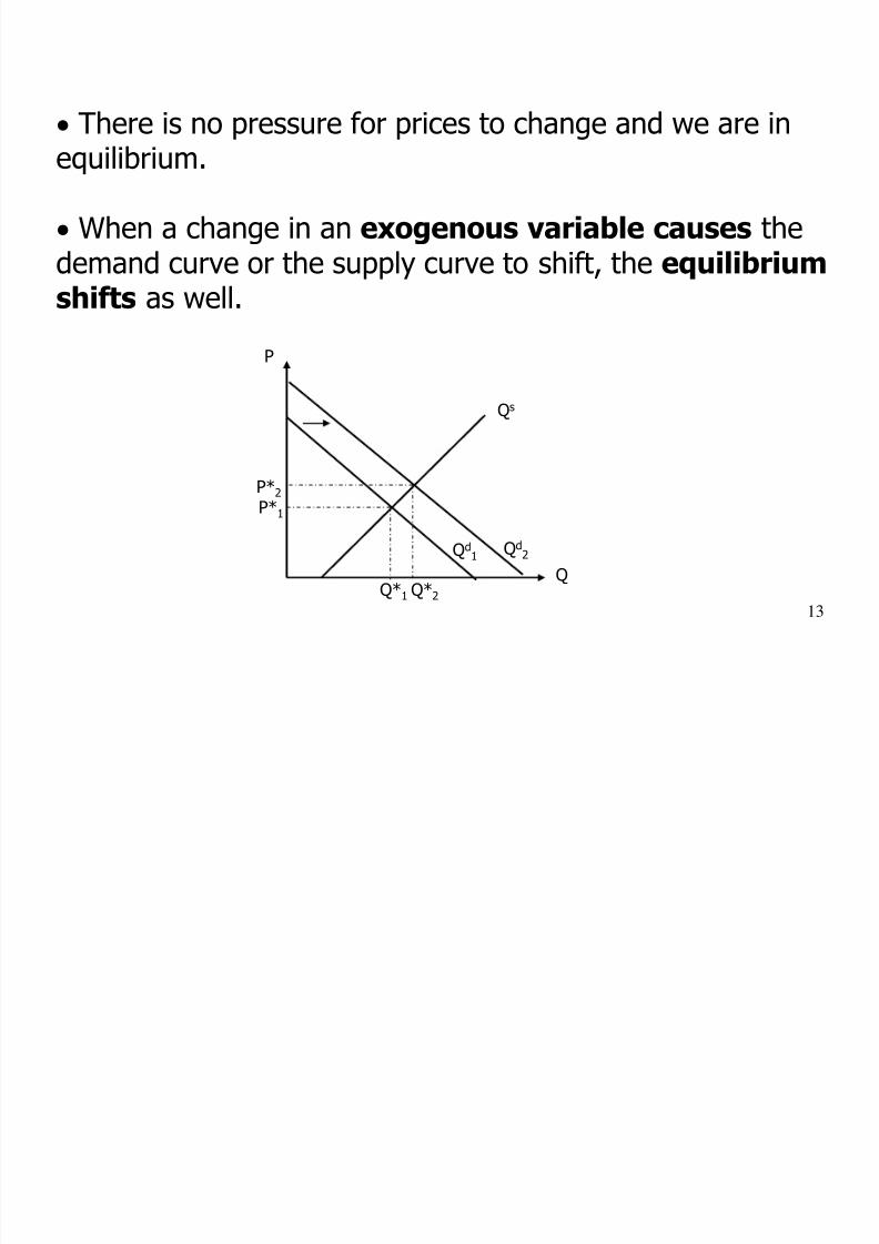
There is no pressure for prices to change and we are in

equilibrium.

When a change in an exogenous variable causes thedemand curve or the supply curve to shift, the equilibrium

shifts as well.P

Q

Qs

Qd1

P*1

Q*1

Qd2

Q*2

P*2



14

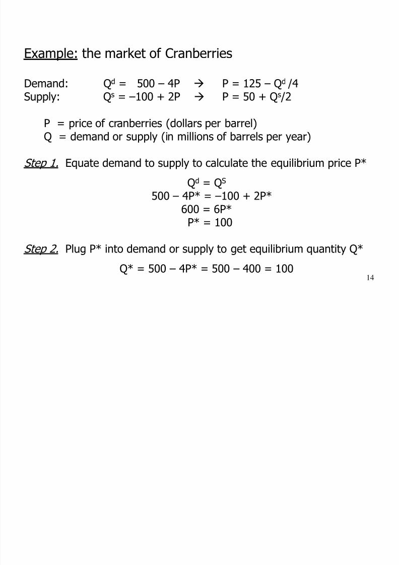
Example: the market of Cranberries

Demand: Qd = 500 – 4P P = 125 – Qd /4Supply: Qs = –100 + 2P P = 50 + Qs /2

P = price of cranberries (dollars per barrel)

Q = demand or supply (in millions of barrels per year)

Step 1. Equate demand to supply to calculate the equilibrium price P*

Qd = QS 500 – 4P* = –100 + 2P*

600 = 6P*P* = 100

Step 2. Plug P* into demand or supply to get equilibrium quantity Q*

Q* = 500 – 4P* = 500 – 400 = 100



15

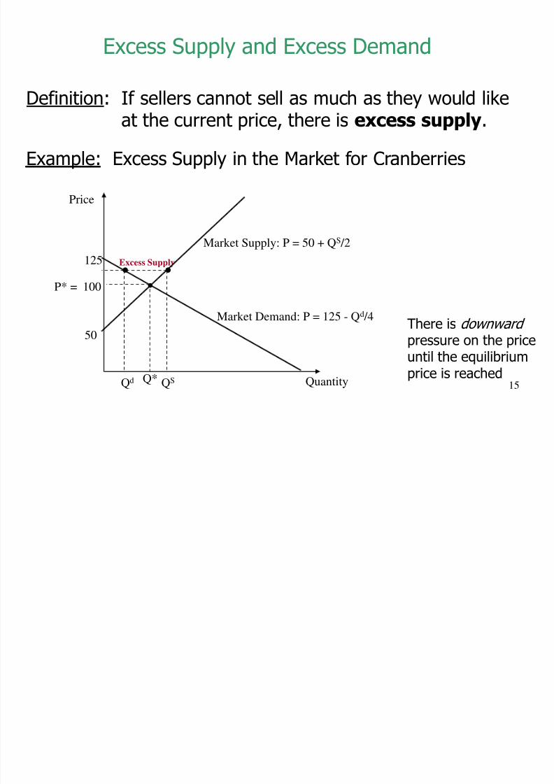
Definition: If sellers cannot sell as much as they would likeat the current price, there is excess supply.

Example: Excess Supply in the Market for Cranberries

Excess Supply and Excess Demand

There is downward pressure on the priceuntil the equilibriumprice is reached

Price

Quantity

Market Demand: P = 125 - Qd /4

Market Supply: P = 50 + QS /2

Q*

50

125 Excess Supply

•

•

QS

Qd

P* = 100

•



16

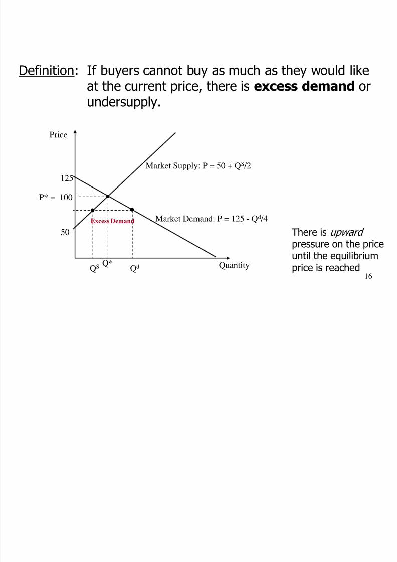
Definition: If buyers cannot buy as much as they would likeat the current price, there is excess demand orundersupply.

Price

Quantity

Market Demand: P = 125 - Qd /4

Market Supply: P = 50 + QS /2

Q*

50

125

Excess Demand

• •

QS Qd

P* = 100

• There is upward pressure on the priceuntil the equilibriumprice is reached



17

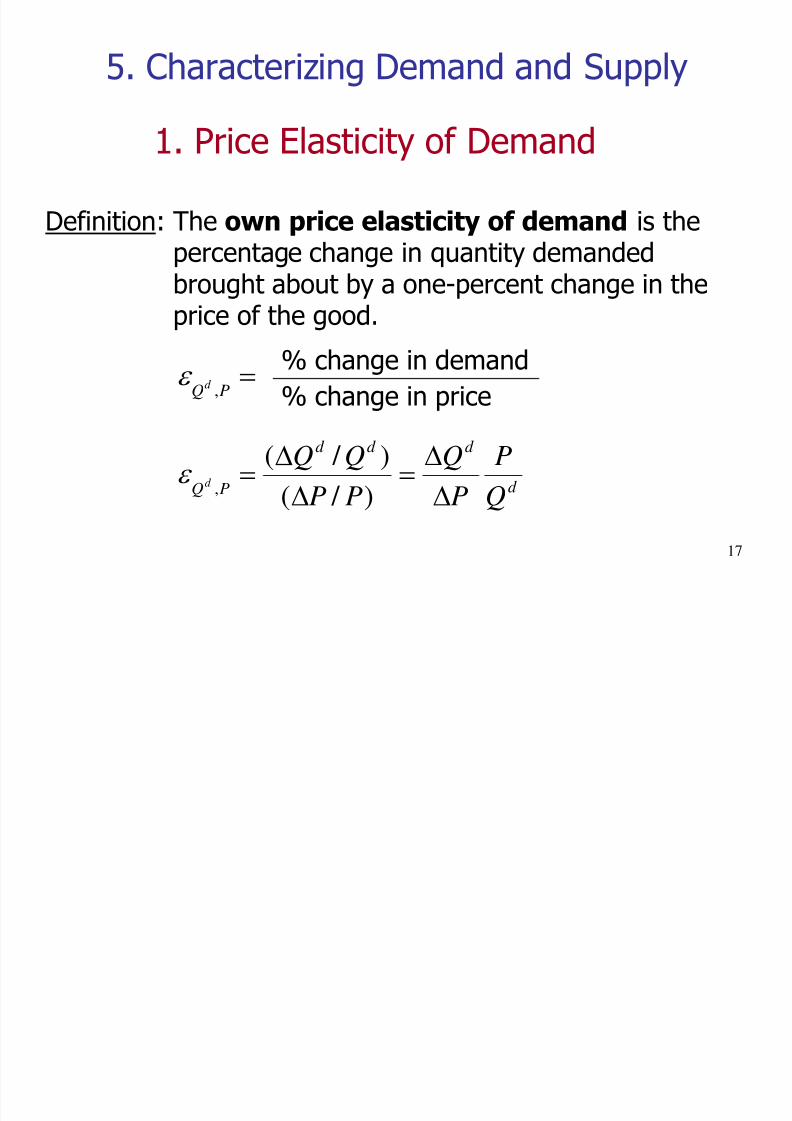
Definition: The own price elasticity of demand is thepercentage change in quantity demanded

brought about by a one-percent change in theprice of the good.

% change in demand

% change in price

5. Characterizing Demand and Supply

1. Price Elasticity of Demand

d

d d d

PQ Q

P

P

Q

PP

QQd

) / (

) / (,

PQ

d ,



18

• The own price elasticity of demand is always negative(or zero)

• The price elasticity of demand plays an important role

in business decisions: it determines the effect on totalrevenue due to a price increase

• Note: Elasticity is not simply equal to slope !

• Slope is the ratio of absolute changes in quantity and price,ie , Qd /P.

• Elasticity is the ratio of relative changes in quantity and price,ie , (Qd /Qd)/(P/P).



19

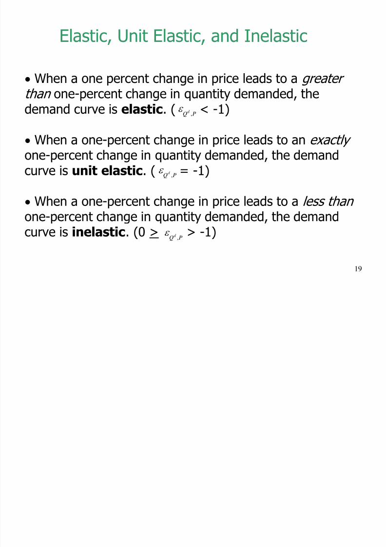
When a one percent change in price leads to a greater than one-percent change in quantity demanded, thedemand curve is elastic. ( < -1)

When a one-percent change in price leads to an exactly one-percent change in quantity demanded, the demandcurve is unit elastic. ( = -1)

When a one-percent change in price leads to a less than one-percent change in quantity demanded, the demandcurve is inelastic. (0 > > -1)

Elastic, Unit Elastic, and Inelastic

PQd ,

PQd ,

PQd ,



20

• In general: the price elasticity of demand depends onthe P and Q we are measuring it in

• Compare 2 functions (take linear demand curves)

P

QQd

A

P1

QdB

P2 P

Bd Q

Ad

Q

The flatter the demand curve,

the more price elastic the demand



21

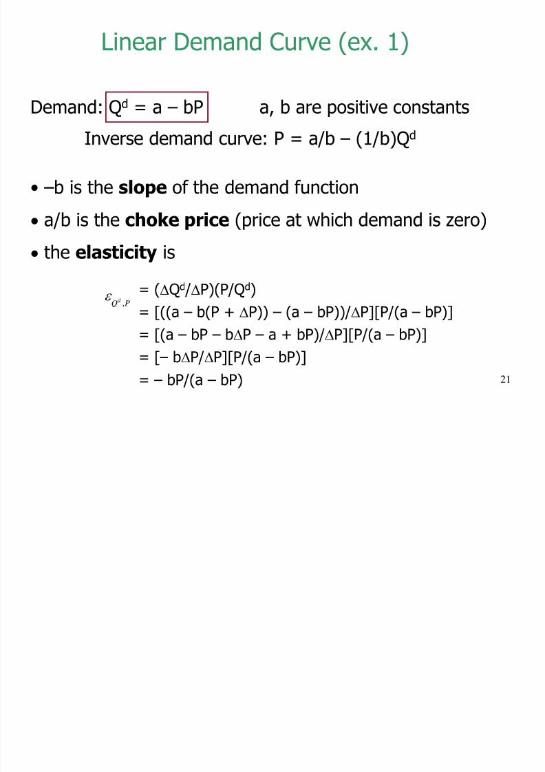
Demand: Qd = a – bP a, b are positive constants

Inverse demand curve: P = a/b – (1/b)Qd

• –b is the slope of the demand function a/b is the choke price (price at which demand is zero)

the elasticity is

= (Qd /P)(P/Qd)= [((a – b(P + P)) – (a – bP))/P][P/(a – bP)]

= [(a – bP – bP – a + bP)/P][P/(a – bP)]

= [ – bP/P][P/(a – bP)]

= – bP/(a – bP)

Linear Demand Curve (ex. 1)

PQd ,



22

0

P

Qa/2 a

a/2b

a/b

• Q,P = -1

Inelastic region

Elastic region

Q,P = -

Q,P = 0

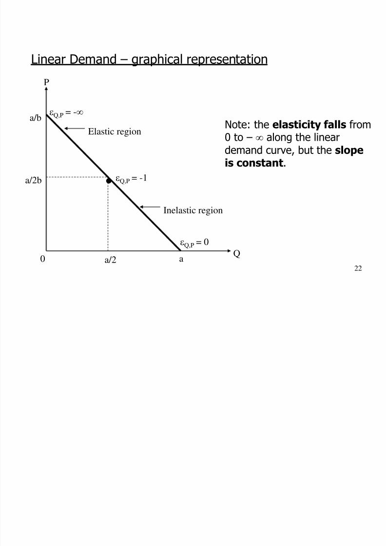
Linear Demand – graphical representation

Note: the elasticity falls from

0 to – along the lineardemand curve, but the slopeis constant.



23

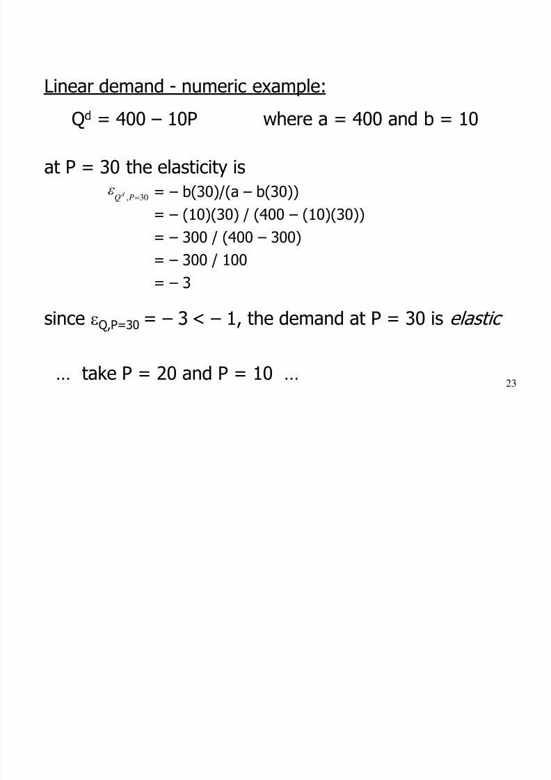
Linear demand - numeric example:

Qd = 400 – 10P where a = 400 and b = 10

at P = 30 the elasticity is

= – b(30)/(a – b(30))= – (10)(30) / (400 – (10)(30))

= – 300 / (400 – 300)

= – 300 / 100

= – 3

since Q,P=30 = – 3 < – 1, the demand at P = 30 is elastic

… take P = 20 and P = 10 …

30, PQd



24

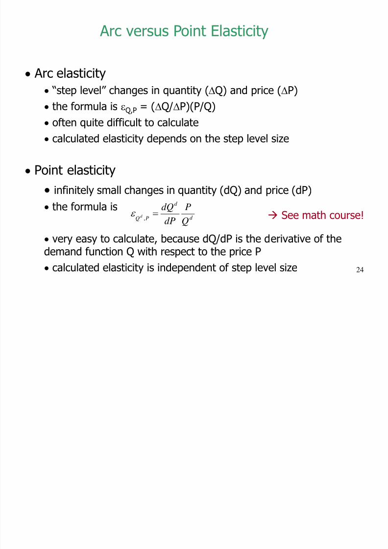
Arc elasticity “step level” changes in quantity (Q) and price (P)

the formula is Q,P = (Q/P)(P/Q)

often quite difficult to calculate

calculated elasticity depends on the step level size

Point elasticity

infinitely small changes in quantity (dQ) and price (dP)

the formula is

very easy to calculate, because dQ/dP is the derivative of thedemand function Q with respect to the price P

calculated elasticity is independent of step level size

Arc versus Point Elasticity

d

d

PQ Q

P

dP

dQd ,

See math course!



25

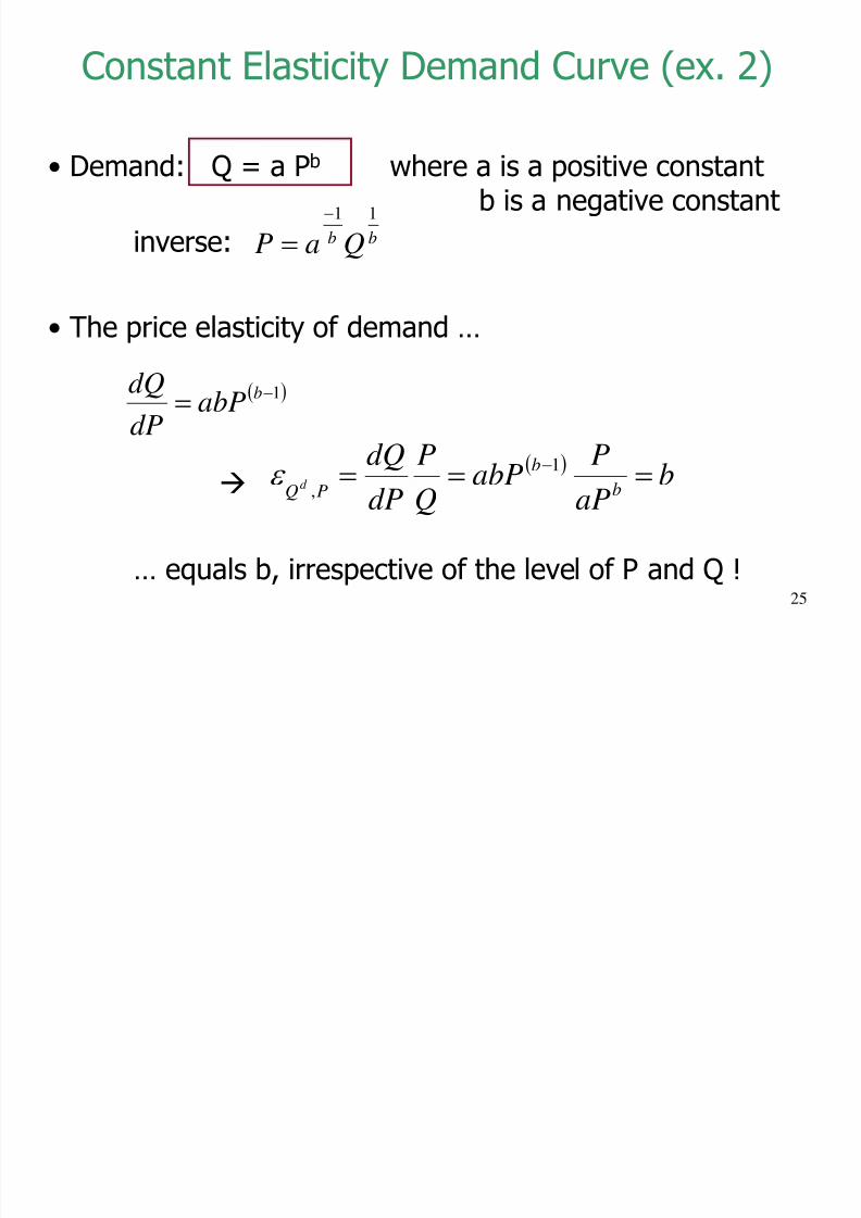
• Demand: Q = a Pb where a is a positive constantb is a negative constant

inverse:

• The price elasticity of demand …

… equals b, irrespective of the level of P and Q !

Constant Elasticity Demand Curve (ex. 2)

bb QaP

11

1

babP

dP

dQ

b

aPPabP

QP

dPdQ

b

b

PQd

1

,



26

Quantity

Price

0 Q

P•

Observed price and quantity

Constant elasticity demand curve

Linear demand curve

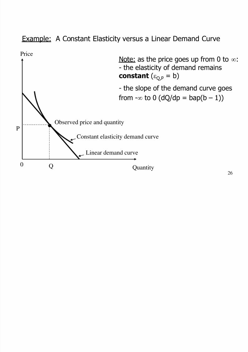
Example: A Constant Elasticity versus a Linear Demand Curve

Note: as the price goes up from 0 to :- the elasticity of demand remainsconstant (Q,P = b)

- the slope of the demand curve goesfrom - to 0 (dQ/dp = bap(b – 1))



27

Examples of factors that can affect own price elasticity:

• substitutability

• switching cost

• product differentiation• example: demand for all soft drinks is less elastic thandemand for Coca-Cola

• durability• definition: a durable good provides valuable services overa long time (usually many years)

• demand for durable goods is relatively elastic in the shortrun, because consumers and firms can delay purchase

What affects the Price Elasticity of Demand?



28

Price ($/airplane)

Quantity (aircraft/yr)

Long run demand curve for commercial airplanes

Short run demand curve for commercial airplanes

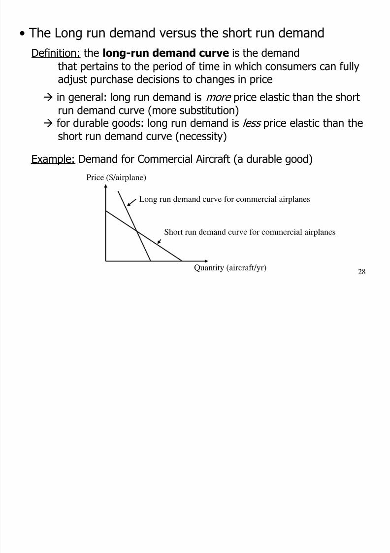
• The Long run demand versus the short run demand

Definition: the long-run demand curve is the demand

that pertains to the period of time in which consumers can fullyadjust purchase decisions to changes in price

in general: long run demand is more price elastic than the shortrun demand curve (more substitution)

for durable goods: long run demand is less price elastic than the

short run demand curve (necessity)

Example: Demand for Commercial Aircraft (a durable good)



29

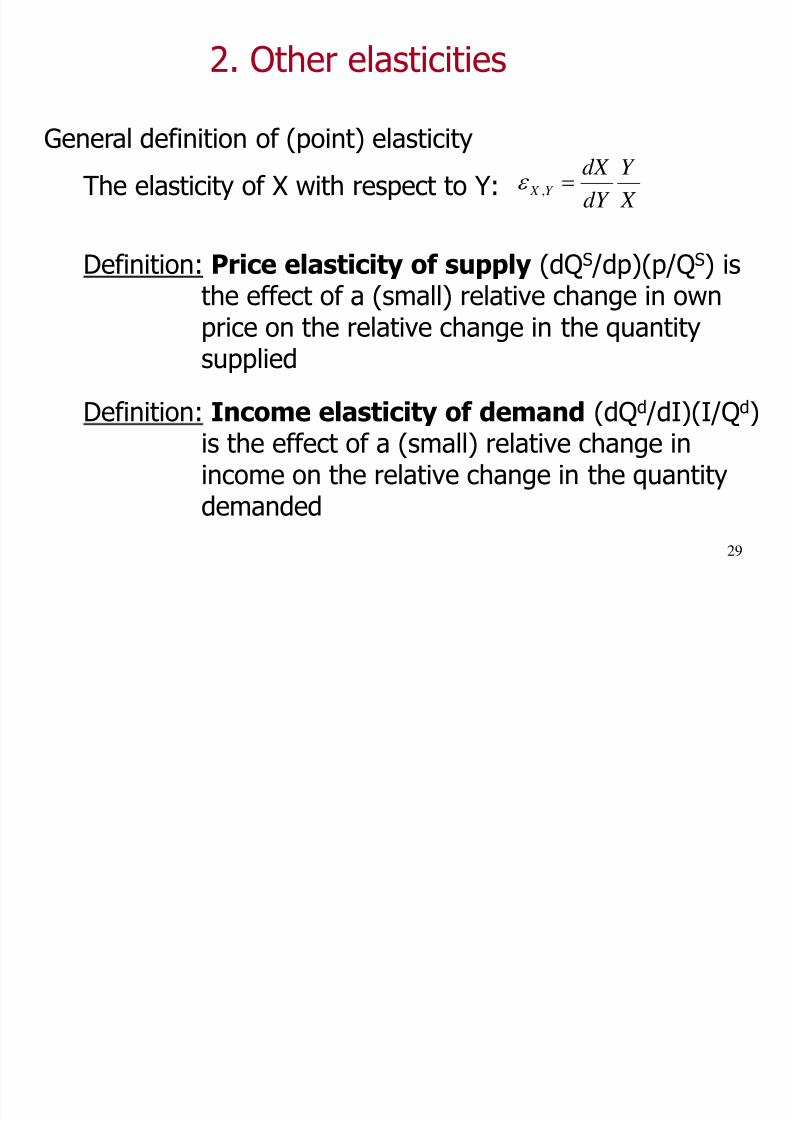
General definition of (point) elasticity

The elasticity of X with respect to Y:

Definition: Price elasticity of supply (dQS /dp)(p/QS) isthe effect of a (small) relative change in ownprice on the relative change in the quantitysupplied

Definition: Income elasticity of demand (dQd

/dI)(I/Qd

)is the effect of a (small) relative change inincome on the relative change in the quantitydemanded

2. Other elasticities

X

Y

dY

dX Y X ,



30

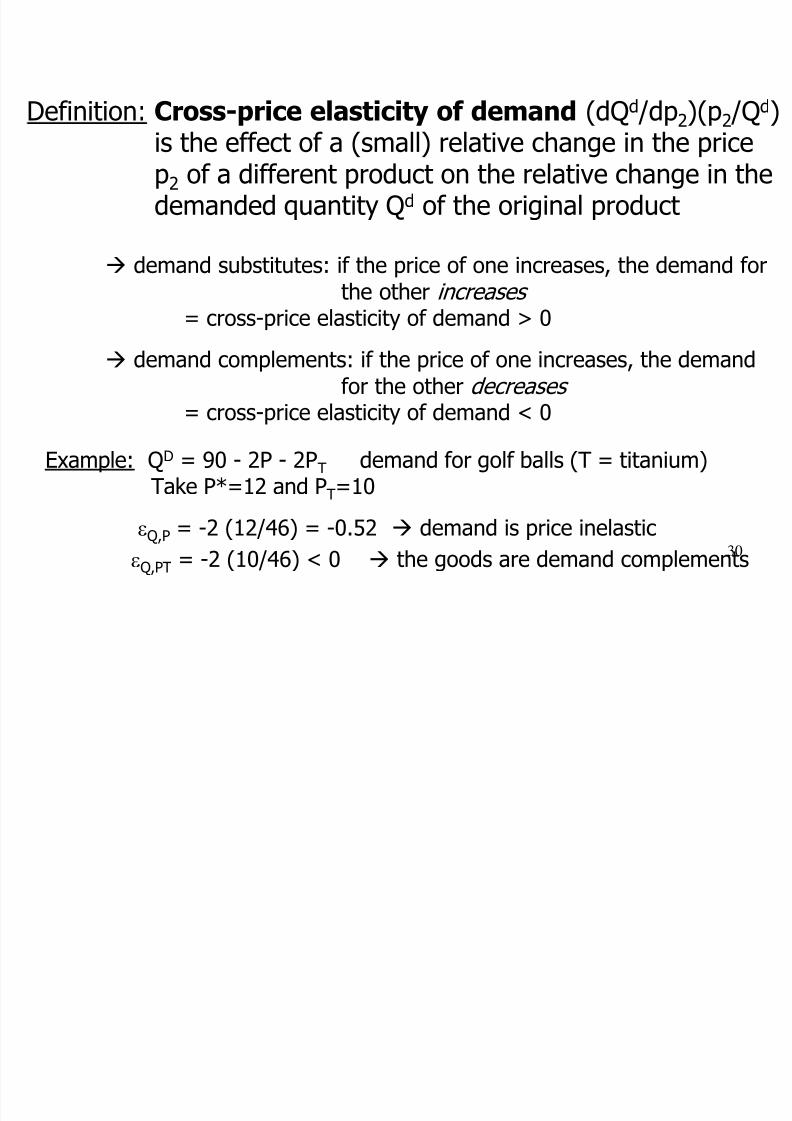
Definition: Cross-price elasticity of demand (dQd /dp2)(p2 /Qd)

is the effect of a (small) relative change in the pricep2 of a different product on the relative change in thedemanded quantity Qd of the original product

demand substitutes: if the price of one increases, the demand for

the other increases = cross-price elasticity of demand > 0

demand complements: if the price of one increases, the demand

for the other decreases

= cross-price elasticity of demand < 0

Example: QD = 90 - 2P - 2PT demand for golf balls (T = titanium)Take P*=12 and PT=10

Q,P = -2 (12/46) = -0.52 demand is price inelastic

Q,PT = -2 (10/46) < 0 the goods are demand complements



31

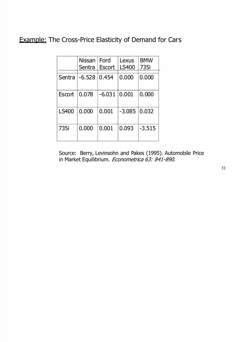
Example: The Cross-Price Elasticity of Demand for Cars

Source: Berry, Levinsohn and Pakes (1995). Automobile Pricein Market Equilibrium. Econometrica 63: 841-890 .

NissanSentra

FordEscort

LexusLS400

BMW735i

Sentra -6.528 0.454 0.000 0.000

Escort 0.078 -6.031 0.001 0.000

LS400 0.000 0.001 -3.085 0.032

735i 0.000 0.001 0.093 -3.515



32

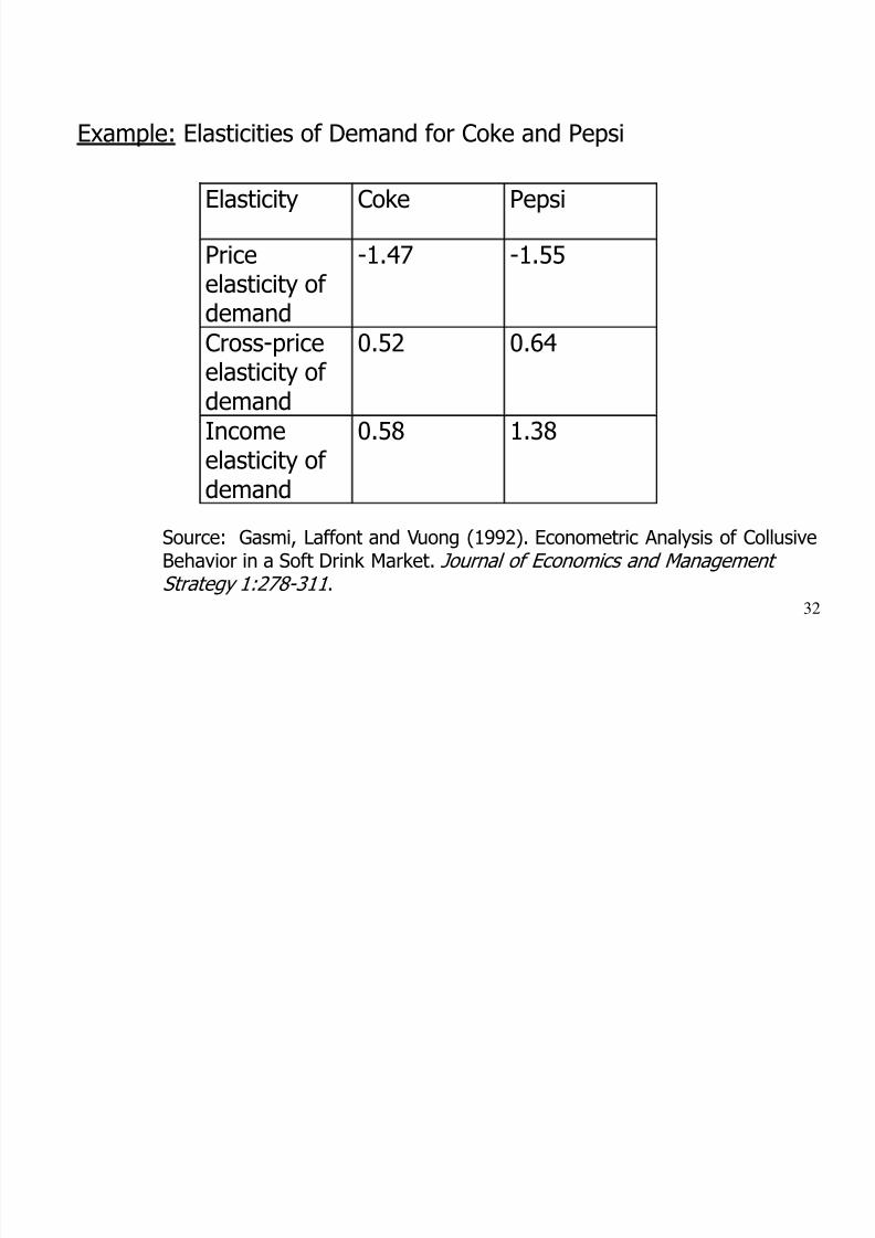
Elasticity Coke Pepsi

Priceelasticity of

demand

-1.47 -1.55

Cross-priceelasticity of demand

0.52 0.64

Income

elasticity of demand

0.58 1.38

Source: Gasmi, Laffont and Vuong (1992). Econometric Analysis of CollusiveBehavior in a Soft Drink Market. Journal of Economics and Management Strategy 1:278-311 .

Example: Elasticities of Demand for Coke and Pepsi



33

1. First example of a simple microeconomic model of supplyand demand (two equations and an equilibrium condition)

2. Elasticity as a way of characterizing demand and supply

3. Elasticity changes as market definition changes(commodity, geography, time)

4. Elasticity a very general concept

02 demand and supply analysis

Documents