0.1 Required Classical Mechanics

The subject of statistical mechanics deals with macroscopic (large sized sys-tems consisting of 1023 particles) systems. As a result, they have a hugenumber of degrees of freedom. These degrees of freedom evolve obeyingnewtons laws of motion, when we are considering a classical statistical me-chanical system. These systems have a very large number of micro-statesdefined by the position coordinates and the momenta of each particle mak-ing up the system. All the micro-states which are consistent to an externallyimposed constraint (like constant energy of the system when its isolated fromthe rest of the universe) actually makes the macro-state of the system. Theequilibrium situation which we will be concerned with in the present courserequires that the probability distribution of the system over these accessible(consistent with the constraint) micro-states is stationary over time.

0.1.1 Hamilton’s equations

Considering a system of N particles (N ∼ 1023), the 3N position coordinatesof the system are denoted by qis, where the suffix i runs over 1-3N, and the 3Nmomenta pis. We consider here the system consisting of particles which donot have other degrees of freedom than translations. These 6N coordinatesat a time t (actually within an interval 4t at the instant t where 4t isarbitrarily small) defines the micro-state of the system at that time t. So, tolook at the evolution of the micro-state we will consider the 6N Hamilton’sequations of the system

pi = −∂H∂qi

(1)

qi =∂H

∂pi(2)

where the dot indicates derivative with respect to time. The Hamiltonian isa function of pi and qi and gives the total energy (T+V) of the system in amicro-state. The existence of the Hamilton’s equations makes the Hamilto-nian stationary in this case i.e. dH

dt= 0.

• Prove that the Hamilton’s equations conserve the Hamiltonian whenits not an explicit function of time i.e. dH

dt= 0.

1

0.1.2 Liouville’s Equation

The micro-state of a system of N particles can be represented by a pointin a 6N dimensional space. The position vector to this phase point X has6N coordinates (in pi and qi) and thus, has all the information about themicro-state under consideration. This space is called the phase space or theΓ-space of the system.

Let us consider the density of the phase points at X in the Γ-space isgiven by f(X, t). This f(X, t) gives a measure of the probability of thesystem to be at the micro-state X, since, having more phase point aroundthe point at X enhances the possibility of the system to visit this point moreoften keeping the system at its neighbourhood for relatively longer time. Thevelocity of the phase points at X is X (remember that the system evolvesaccording to the Hamilton’s equations and one can move along a trajectorypassing through the phase point X given by this dynamics). The elementaryflux through a surface area ds at X is dF = ds · (Xf(X, t)). The total flux(outward by convention) through an arbitrary closed surface S enclosing thevolume V is

F =

∫dF =

∫S

ds · (Xf(X, t)). (3)

This flux has to match the time rate of decrease of the total phase pointsinside the volume V which is ∂

∂t

∫vdvXf(X, t). Equating these tow quantities

and applying the Gauss’s theorem∫Sds · A =

∫VdvO · A for an arbitrary

vector field A ∫V

dvX

(∂f

∂t+ O · Xf

)= 0. (4)

Since, the integration is over arbitrary volume, the integrand must vanish tomake the relationship hold good for all V and that gives

∂f

∂t+ O · Xf = 0. (5)

Now, O · Xf = fO · X + X · Of and it can be shown that O · X = 0when the components of X evolves according to Hamilton’s equations. Thisdivergence less flow is a signature of a Hamiltonian system and it can also beshown from the consideration of a divergence less flow that the phase spacevolume of such a Hamiltonian system remains conserved over time. Imaginethat a phase space volume dvX is evolving in time along the trajectory of thephase points in it towards its later configuration dvfX . The divergence free

2

velocity field of the phase points motion ensures that dvX = dvfX . Contraryto the Hamiltonian systems, in dissipative systems the phase space volumecan change and that is why in dissipative dynamical systems we talk aboutthe attractors in phase space which can be nodes, limit cycles or strangeattractors to which an initial volume of the phase space (basin of attraction)converges to (by getting contracted) at large time.

• Show that O · X = 0 when the system evolves along a Hamiltoniantrajectory.

Thus, the Liouville’s equation for the hamiltonian flow is

∂f

∂t+ X · Of = 0. (6)

0.1.3 Equilibrium and Ensemble

The equilibrium of the system demands no explicit time dependence of thephase space density. Considering ∂f

∂t= 0 modifies eq.6 as X · Of = 0 which

can be rewritten in the form of Poisson’s bracket as f,H = 0. Poisson’sbracket of two functions A and B of pi and qi is the expression

A,B =∑i

(∂A

∂qi

∂B

∂pi− ∂A

∂pi

∂B

∂qi

)(7)

• Prove that X · Of = f,H

The relation f,H = 0 ensures that f = f(H(qi, pi)). So, in the context ofequilibrium statistical mechanics we would always get the probability distri-bution over the micro-states as a function of the hamiltonian. While the prob-ability of the system to be at a micro-state is given by f(H),

∫VdvXf(H) = Z

over the whole accessible phase space is called the partition function and theaverage of any quantity A is given as

< A >=

∫VdvXAf(H)

Z(8)

which indicates that the average would not change even if f(H) = Cf(H)where C is an arbitrary constant.

At equilibrium, the system under consideration generally satisfies certainmacroscopic constraints like the total energy of the system is a constant or the

3

temperature of the system is constant etc. which actually defines the macro-state. The stationarity of the probability distribution over the phase spacef(H) ensures that if we prepare a large number of similar systems, called anensemble, which are subject to the same macroscopic constraint, then, themicro-states of these systems at an instant of time will be distributed over thephase space according to the probability distribution on it. Thus, averagingover these collection of systems at an instant is equivalent to time averagingover a larger period of time, since, given that time the system would visitall the points in phase space where the ensemble is sitting at an instant inaccordance with the same probability distribution.

0.2 Micro-canonical Ensemble

In micro-canonical ensemble we consider an isolated system. The relevantconstraint on the system is its total energy E which is practically a constantdue to lack of interactions and we generally take the energy to remain withina very small range δE at E so that E ≤ H(pi, qi) ≤ (E + δE). Let ushave an estimate of the phase space volume accessible to a system of N noninteracting classical particles. If we consider that all of those N particlesare identical then a transformation that exchanges the positions of any pairof particles will produce a new phase point in the Γ-space (because particleidentifying indices are included in the suffix of ps and qs), but the actualmicro-state will be identical to the previous one. Consequently, we actuallyhave to alter the phase space density f(H) to f(H) = C ′ f(H)

N !to correct the

over counting of the actual micro-states1. Here C ′ is an arbitrary constanttaking care of all other relevant things.

The probability distribution function for micro-canonical ensemble weconsider is in the form f(H) = Cδ(E −H) where δ(E −H) is a Dirac deltafunction and the N! term has been absorbed in the new constant C. We wantto find the partition function of an isolated system of classical particles which

1The N! takes care of so called Gibb’s Paradox (see Pathria)

4

are non interacting (classical ideal gas).

Z = C

∫dvXδ(E −H(p, q))

= C

∫ 3N∏i=1

dqi

3N∏j=1

dpjδ(E −H(pj, qi))

= CV N

∫R=2m

√E

3N−1∏j=1

dp′j. (9)

In the above expression V is the volume of the container and the volumeterm originates from the integration over qis. Since, the constraint here is onthe kinetic energy (potential energy is zero by consideration), the constraintwill actually be felt on the momentum space. The removal of the deltafunction from the integral is justified by adjustment of the integration limitswhich takes care of the energy constancy. To do that we have moved to acoordinate system which is a spherical polar analogue of 3-D in 3N-D and theradial coordinate of such a system R will be given generally as R2 =

∑3Nj=1 p

2j .

But, E =P3Nj=1 pj

2mwhere m is the mass of each particle, readily produces the

radius of the constant energy surface R = 2m√E on which all the momentum

micro-states of the system should fall. A ’′’ to the pj coordinates in the lastline of eq.9 indicates that they are now different coordinates (angle like) thanthose in the previous line. So, the result of the remaining integration in theeq.9 is the surface area of the (3N-1) dimensional sphere. General formula for

the surface area of an n-1 dimensional sphere is An = 2 πn/2

Γ(n/2)R(n−1). So, in the

present case the value of the momentum integral is 2 π3N/2

Γ(3N/2)(2m)3N−1E

3N−12 .

Z = CV N(2m)3N−1E3N−1

2 (10)

where all the constants have now been absorbed in the constant C.Let us look at the calculation of the partition function more closely. It

involved calculating the accessible phase space volume Ω to the system un-der consideration and Z is actually proportional to the Ω. The constant ofproportionality which enters via the presence of C is at most a function ofthe particle number N and not of E and V. So, from the calculation of Zwe can easily conclude that Ω = Ω(E, V,N). A measure of entropy due toBoltzmann is S = kBlog(Ω) where kB is Boltzmann constant which has a

5

value 1.38× 10−16 erg/K. This definition of entropy is a bridge between themicroscopic and the macroscopic domains and using this definition we canactually get to the macroscopic thermodynamic relations from the knowledgeof the microscopic evolution of the system.

Ω being a function of E, N and V makes S a function of the same variablesin the micro-canonical case. Consider a variation of S

dS =

(∂S

∂E

)V,N

δE +

(∂S

∂V

)N,E

δV +

(∂S

∂N

)E,V

δN. (11)

The conservation of energy requires the increase in energy of a system δEbe equal to the amount of heat given to it δQ and the work done on itδW . Thermodynamic definition of entropy gives us δQ = TdS where Tis the temperature of the system. δW = −PδV + µδN , where −PδV isthe work done on the system and µδN is the work done on the system byaddition of particles where µ is the chemical potential of the system. Thus,the conservation of energy expresses the increment in entropy as

dS =

(1

T

)δE +

(P

T

)δV −

(µT

)δN. (12)

Equating the coefficients of Eq.11 and Eq.12 we get the thermodynamic re-lations as (

∂S

∂E

)V,N

=1

T(∂S

∂V

)N,E

=P

T(∂S

∂N

)E,V

= −µT

Its interesting to note that Ω being the phase space volume of the sys-tem in 6N-1 dimensional space (constant energy constraint H = E reducesone dimension) is actually a constant energy surface (spherical since R is afunction of E) in 3N dimensions. Now, consider that E ≤ H ≤ (E +4). Inthis case, the phase volume accessible to the system (spatial part is fixed byfixing the volume of the system) falls within the annular region between thetwo constant-energy surfaces giving us

Ω×4 = Σ(E +4)− Σ(E) (13)

6

where Σ(E) is the phase volume accessible to the system for all energies lessthan equal to E. Now, taking the limit 4→ 0, Ω is recognized as the densityof states at the energy E with an expression Ω = ∂Σ(E)

∂E. Since, log(Ω) differs

from log(Σ(E)) by an additive function of N the definition of the entropy asS = kBlog(Σ) is equivalent to that with respect to Ω. Both of these entropiesgive the same temperature and retains the extensive property of it.

• Show that log(Ω) differs from log(Σ(E)) by an additive function of Nin the case of classical ideal gas.

0.2.1 Micro-canonical derivation of virial theorem

The mathematical statement of the virial theorem states that < xi∂H∂xj

>=

δijkBT . The average here is done on micro-canonical ensemble

< xi∂H

∂xj> =

1

Ω

∫ ∏i

dpidqi

(xi∂H

∂xj

)δ(E −H)

=1

Ω

∂

∂E

∫H<E

∏i

dpidqi

(xi∂H

∂xj

)=

1

Ω

∂

∂E

∫H<E

∏i

dpidqi

(∂xi(H − E)

∂xj− δij(H − E)

)

=1

Ω

∂

∂E

(∫ surface

H∼Edp′idq

′ixi(H − E)−

∫H<E

∏i

dpidqiδij(H − E)

)(14)

In the last line of the above expressions, the first integral is now the onewhich is an integration over the surfce of 6N-1 dimensions. This we get byintegrating over the xj coordinate on a spherical polar frame and the restof the coordinates are now like angles (effectively) which define the constantenergy surface (H − E). The prime on the coordinates pi and qi actuallyindicates of the fact that they are different in nature than those in the pre-vious line2. The first integral (surface one) actually vanishesh since (H=E)

2this is not at all necessary if we keep in mind that from the very beginning we are ona polar frame

7

on it. So,

< xi∂H

∂xj> =

1

Ω

∂

∂E−∫H<E

∏i

dpidqiδij(H − E)

=1

Ωδij

∫H<E

∏i

dpidqi.

Thus,

< xi∂H

∂xj>= δij

Σ(E)

Ω= δij

kBkB∂ln(Σ(E))

∂E

= δijkB∂S∂E

= δijkBT (15)

The measure of average K.E. per degrees of freedom can readily be got fromthe expression < xi

∂H∂xj

>= δijkBT which shows < piqi2>= 1

2kBT which is the

average K.E. per degree of freedom.

0.3 Canonical Ensemble

In canonical ensemble we take into consideration the statistical mechanicsof a system which is in thermal contact with a reservoir of heat. The heatreservoir is much much bigger than the system itself so that exchange of heatto the system does not alter the temperature of the reservoir. The systembeing in thermal equilibrium shares the same temperature with its reservoir.Let the system be denoted by A and the reservoir by A′ and together theymake a micro-canonical system A0 = A + A′. Given the total energy ofthe A0 as E0, the individual energies of the system and its reservoir E andE ′ respectively add up to give E0. When the system is at an energy E, theprobability of the system to be at this state is proportional to the compatiblemicro-states available in its environment to keep it stay at this energy E i.e.Ω(E ′). Expanding ln(Ω(E ′)) = ln(Ω(E0 − E)) about E0 we get

ln(Ω(E0 − E)) = ln(Ω(E0))−(∂Ω(E ′)

∂E

)E = ln(Ω(E0))− E

kBT. (16)

Thus the probability of the system to be at the energy state E, P (E) is pro-portional to e−βE where β = 1/kBT (T is the temperature of the reservoirwhich is also the temperature of the system when it is in thermal equilibriumwith the reservoir). So, from now on we will take P (E) = e−βE/ΣEe

−βE, the

8

constant of proportionality is taken care of by the normalization. The nor-malization constant ΣEe

−βE is generally known as the partition function ofthe system (exactly as in the micro-canonical case). Let us get a few pointscleared in the beginning. The energy E actually contains the kinetic and thepotential parts. But equipartition of energy, where applicable, makes theaverage energy per degrees of freedom a function of temperature only. Tem-perature of a system being in canonical equilibrium (classical) is a constantand as a result gets cancelled by normalization. Its only the potential energyof the system which features in the expression of the probability. Consider thestate of the system at energy E to be degenerate. If there are nE states at theenergy E then the probability of the system to be at energy must get nE foldraised. So the probability will now be P (E) = nEe

−βE/ΣEnEe−βE. In the

continuum, its the density of states Ω(E) that gives you the measure of the nEbecause by definition density of states is the number of states at the energy E.Thus, in continuum, the probability is P (E) = Ω(E)e−βE/

∫dEΩ(E)e−βE.

The relation which is used to bridge the statistical mechanics to thethermodynamics in the canonical ensemble case is the partition functionZ = e−βF where F is the Helmholtz free energy (relevant thermodynamicpotential in the canonical case) and thermodynamically F =< E > −TS.The < E > in the expression of F is canonical average energy defined as

< E >=

∑Ee−βE

Z. (17)

Taking the derivative with respect to β the average energy is given by <E >= −∂ln(Z)

∂β. The dispersion of the system < 4E2 >=< E2 > − < E >2

is given by -∂<E>∂β

indicates that the average energy always increases withtemperature to keep the dispersion positive definite. To get to the expressionof the dispersion let us consider

< E2 >=1

Z

∑ ∂2

∂β2e−βE =

∂

∂β

(1

Z

∑ ∂

∂βe−βE

)+

(∑∂∂βe−βE

)2

z2(18)

So, using the expression of < E >,

< 4E2 >= −∂ < E >

∂β. (19)

The generalized force of a system is negative gradient of energy and fol-lowing this rule, the generalize force corresponding to the thermodynamic

9

coordinate x (also called parameter) is −∂E∂x

. so the work done by the systemunder the action of this force to achieve a displacement of dx is

dw = −∑

∂∂xe−βE

Z× dx =

1

β

∂ln(Z)

∂x× dx. (20)

Now, consider the partition function to be a function of the coordinate x andtemperature β. Given that, an increment of ln(z) is written as

d(ln(Z)) =∂ln(Z)

∂xdx+

∂ln(z)

∂βdβ = βdw − d(< E > β) + βd < E > (21)

or

d(ln(Z) + β < E >) =dS

kB(22)

Thus, we arrive at the relation which combines canonical stat. mech. tothe thermodynamics and the relation is Z = e−βF where F =< E > −TS isthe Helmholtz free energy.

0.3.1 Gaussian form

As we know the probability distribution of a system over an energy scale(continuum) is given by P (E) = Ω(E)e−βE, the Ω(E) part of the probabilityis a very rapidly increasing quantity of energy whereas the e−βE is a rapidlydecreasing function of E. A combination of rapidly increasing and rapidlydecreasing parts make the probability P(E) have a peak at some Em on thescale where Em is the most probable energy of the system. Since Em is themaximum of the distribution the following relation holds.[

∂

∂E

(e−βEΩ(E)

)]E=Em

= 0, (23)

which immediately gives [∂ ln Ω(E)

∂E

]E=Em

= β. (24)

Now, from the Eq.22 and considering the relation s = kb ln Ω(E) we get

1

kB

[∂S

∂E

]E=<E>

= β =

[∂ ln Ω(E)

∂E

]E=<E>

(25)

10

Eq.24 and 25 are the same relations but derived at E = Em and E =< E >,which indicated that Em =< E > and the P (E) is a symmetric distributionabout the most probable value of it which is the same as the average of thedistribution i.e. < E >.

Having know that the P (E) is symmetric, let us try to find its actualshape. To that end, consider the lnP (E) and expand it on a Taylor seriesabout < E >.

ln(Ω(E)e−βE

)= ln

(Ω(< E >)e−β<E>

)+

1

2

[∂2Ω(E)e−βE

∂E2

]E=<E>

(E− < E >)2 + higherorderterms.

(26)

The first derivative does not appear in the above expression due to the factthat < E > coincides with Em and consequently the first derivative is zero atE =< E >. Now, using the thermodynamics relations we have encounteredso far, one can easily show that the first (constant) term on the r.h.s. of theabove equation can be writte as −β(< E > −TS), and, the coefficient ofthe second term in (E− < E >)2 can be expressed as −1/2kBT

2CV . Usingthese thermodynamic expressions one can write the form of P (E) down as

P (E) = e−βF × e−(E−<E>)2

2kBT2CV (27)

• Arrive at Eq.27 starting from Eq.26 using required thermodynamicrelations.

Equation 27 manifests a Gaussian form for the probability distribution func-tion P (E) which has a width or standard deviation σ = T

√kBCV where CV

is the specific heat of the system at constant volume. The CV is an extensivequantity i.e. it scales as the number of particles (molecules) N in the sys-tem. This can easily be understood from the definition of CV which is theamount of heat required to raise the temperature of the system by one de-gree. Since the temperature is a measure of the average K.E. of the particlesin the system CV should scale as N . The energy of the system < E > is alsoan extensive quantity i.e. proportional to N. So, σ/ < E >∼ N

12 . In the

thermodynamic limit, as N → ∞ the distribution becomes infinitely sharpon the scale of < E >.

11

0.3.2 Correspondence between micro-canonical and canon-ical ensembles

At the thermodynamic limit, considering the probability distribution to be adelta function about its average energy, the partition function, which is thearea under the probability distribution curve on energy scale, can be writtenas

Z ' Ω(< E >)e−β<E> × δElnZ = lnΩ(< E >)− β < E > (neglecting ln δE). (28)

The above expression of lnZ when combined to the other expression Z =e−βF immediately leads us to the relation

S = kB ln Ω(< E >). (29)

But, this is the definition of micro-canonical entropy which we have arrivedat from the canonical distribution at thermodynamic limit. This observationimplies the correspondence or equivalence of canonical and micro-canonicalensembles at the thermodynamic limit and one may use either of them de-pending upon the amount of ease it provides in dealing with the mathematics.Generally, using canonical ensemble makes life simple by not putting any re-striction on the integration limits and one can integrate up to the extremelimits of the phase space variables (degrees of freedom) or the energy wherethe canonical distribution function takes care of the irrelevant extensions overthese scales with the help of some useful potential functions (or functionals)of the degrees of freedom.

0.3.3 Alternative expression of entropy

Let us derive an expression of entropy, useful in the context of canonicalensemble, starting from the expression of the canonical partition function

12

lnZ = −β(< E > −TS).

S = kB

[lnZ + β

∑i

PiEi

]

= kB

[lnZ −

∑i

Pi ln (ZPi)

]

= kB

[lnZ − lnZ

∑i

Pi −∑i

Pi lnPi

]Since,

∑i Pi = 1, we get

S = −kB∑i

Pi lnPi (30)

This is the expression of entropy for a canonical ensemble which is positiveon account of the fact that Pi is a fraction.

0.3.4 Canonical distribution by entropy maximization

Let us have a look at an alternative derivation of canonical distribution func-tion to correlate the equilibrium distribution with the maximization of en-tropy of the system. Consider a large number ’a’ of similarly prepared sys-tems which are in contact with a heat reservoir and the average energy overall these systems is ¡E¿ a constant. Thus,∑

i

ai = a = constant∑i

δai = 0 (31)

and ∑i

aiEi =< E >= constant∑i

δaiEi = 0 (32)

Eq.31 and 32 are the two constraints on the variation of number of elementsof the ensemble at an energy Ei. Consider the number Γ(a1, a2, ..., an) in

13

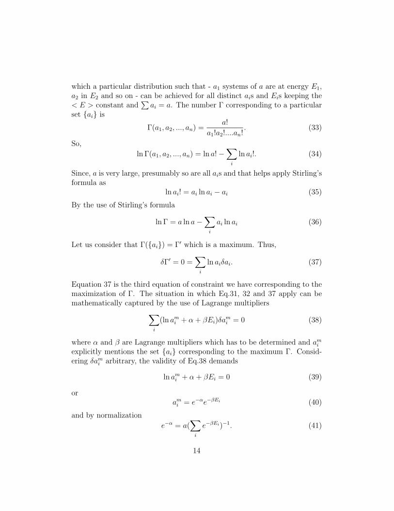
which a particular distribution such that - a1 systems of a are at energy E1,a2 in E2 and so on - can be achieved for all distinct ais and Eis keeping the< E > constant and

∑ai = a. The number Γ corresponding to a particular

set ai is

Γ(a1, a2, ..., an) =a!

a1!a2!....an!. (33)

So,

ln Γ(a1, a2, ..., an) = ln a!−∑i

ln ai!. (34)

Since, a is very large, presumably so are all ais and that helps apply Stirling’sformula as

ln ai! = ai ln ai − ai (35)

By the use of Stirling’s formula

ln Γ = a ln a−∑i

ai ln ai (36)

Let us consider that Γ(ai) = Γ′ which is a maximum. Thus,

δΓ′ = 0 =∑i

ln aiδai. (37)

Equation 37 is the third equation of constraint we have corresponding to themaximization of Γ. The situation in which Eq.31, 32 and 37 apply can bemathematically captured by the use of Lagrange multipliers∑

i

(ln ami + α + βEi)δami = 0 (38)

where α and β are Lagrange multipliers which has to be determined and amiexplicitly mentions the set ai corresponding to the maximum Γ. Consid-ering δami arbitrary, the validity of Eq.38 demands

ln ami + α + βEi = 0 (39)

orami = e−αe−βEi (40)

and by normalization

e−α = a(∑i

e−βEi)−1. (41)

14

Once we know the expression of ami we an readily find out the correspondingprobability distribution function and average energy

Pi =amia

=e−βEi

e−βEi(42)

< E >=

∑i e−βEiEi

e−βEi(43)

Eq.42 is the canonical distribution we have already got. Since, all the el-ements of the ensemble are in contact with the same heat bath the otherLagrange multiplier β is equal to 1/kBT , where T is the temperature of thebath, from analogy. Thus, the canonical distribution function is arrived aton maximization of the number Γ at a constant average energy of a fixedsized ensemble. To relate Γ to the entropy of the system rewrite Eq.36 as

ln Γ = a ln a−∑i

aPi ln aPi

= a ln a− a∑i

Pi(ln a+ lnPi)

= a ln a− a ln a(∑i

Pi)− a∑i

Pi lnPi

ln Γ = −a∑i

Pi lnPi

Thus, ln Γ is proportional to the canonical entropy ln Γ = akBS and maxi-

mization of Γ is equivalent to the maximization of the entropy of the system.So, in canonical equilibrium the entropy of the system is a maximum corre-sponding to a constant average energy and temperature of the system. TheHelmholtz free energy of the system F =< E > −TS would definitely be aminimum when entropy is a maximum at constant < E > and T and theequilibrium thermodynamic relations are subject to these extremum condi-tions. The maximization of entropy can be understood as a consequenceof maximizing the symmetry of the system at the microscopic level wherethe thermal equilibrium would ensure no further evolution of the probabil-ity distribution of the system towards any more symmetric situations. Therequirement of the highest symmetry is a consequence of thermalization ofthe system and corresponding disorder. The level of microscopic disorder issimilar to the level of symmetry of the system at the microscopic level andit comes out that the system tries to remain maximally disordered to fix theprobability distribution to a stationary profile.

15

0.4 Grand canonical ensemble

The grand canonical ensemble represents systems which are in contact withan environment with which it can exchange heat and particles as well. So,unlike canonical ensemble the total number of particles is not a constant forsuch systems, rather the energy and particle numbers both can vary. Follow-ing a similar treatment as the one used to arive at the canonical distributionfunction we can derive the probability distribution function for the grandcanonical system i.e. the probability of the system to be at an energy Eiwith number of particles Nj as

Pij = e−β(Ei−µNj/ZG. (44)

The ZG =∑

ij e−β(Ei−µNj) is grand partition function and is related to the

thermodynamics of the system through the relation

lnZG =PV

kBT(45)

which basically is equation of states. The Gibbs potential G = F + PVis the relevant thermodynamic potential in the grand canonical case. Theuse of it we will come accross at the time of discussing phase co-existence ofsystems. Gibbs potential is a function of temperature, pressure and numberof particles of the system i.e. G=G(T,P,N). Take the definition of G asF + PV . A variation in it is then expressed as

dG = dF + PdV + V dP = d < E > −TdS − SdT + PdV + V dP, (46)

the last equality follows from the definition of the Helmholtz potential F =<E > −TS. Now, consider the conservation of energy as

d < E >= dQ− PdV + µdN (47)

where the change in internal energy of the system is equal to the sum of heatgiven to it, mechanical work done on it, and the rise in energy of it due toaddition of particles to it. This immediately gives

d < E > +PdV − dQ = d < E > +PdV − TdS = µdN. (48)

Using Eq.48 and Eq.46

dG = µdN − SdT + V dP, (49)

which clearly shows that G=G(T,P,N).

16

0.5 Application of Boltzmann statistics: Maxwell

velocity distribution

Consider a classical gas of noninteracting distinguishable particles. Such aclassical gas limit can be achieved at a high temperature and a very diluteconditions. Since the particles are noninteracting, they only have the K.E.which is equal to p2/2m for the particle having momentum p and the massm. In what follows we will consider the all the particles of mass m. From theknowledge of the Boltzmann distribution function for a system of particlesat a constant temperature T, we can say that the probability for the particleunder consideration to remain at a momentum p within the range dp anda position r within a range dr is f(p, r)d~pd~r ∝ e−βp

22md~pd~r. So, the totalnumber of particles at the momentum p and position r within the ranges dpand dr respectively is

n(p, r)d~pd~r = Ce−βp22md~pd~r (50)

where the proportionality constant would be found out from the considerationof the constraint that the system has N number of particles in a volume V.If one integrates either sides of the above equation, one gets N; thus,

N = CV

∫e−βp

22md~p. (51)

Taking into account p2 = m2(v2x + v2

y + v2z), we can make the change of

variables by absorbing some constants into the constant C (which has to bedetermined.

N

V= n = C

∫e−

βm(v2x+v2y+v2z)

2 dvxdvydvz (52)

Utilizing the symmetry along the x, y, and the z directions one can easily show

that the integral in the above equation is actually equal to

(∫e−

βmv2x2 dvx

)3

=(2πβm

) 32

and thus, C = n(βm2π

) 32 . Finally, the Maxwell velocity distribution

for distinguishable non-interacting classical particles i.e. number of particlesat velocity ~v and within a range d~v reads as

f(~v, r)d~rd~v = n

(m

2πkBT

) 32

e−mv2/2kBTd~vd~r (53)

17

Eq.53 gives a Gaussian distribution with zero mean. If one is interestedin the distribution of speed one has to write the d~v as 4πv2dv, becausein spherical polar coordinate we are effectively, in this way, considering allthe velocities of magnitude v irrespective of their directions. Using thisdifferential form of volume element in the spherical polar coordinates weget the speed distribution function

f(v) = N4πv2

(m

2πkBT

) 32

e−mv2/2kBT . (54)

These speed distribution function is clearly not a Gaussian due to the pres-ence of the v2 term in the coefficient of the exponential part. One can calcu-late all the aerage quantities for such systems considering either of the twodistribution functions shown above.

0.5.1 Equation of state for ideal classical gas

The momentum transferred per unit time in positive x-direction cross thearea dA held perpendicular to the x-direction, in a gas is

F+ =

∫vx>0

d~vf(~v)dA(|~v| cos θ)(m~v) (55)

where dA|~v| cos θ is the volume on the left hand side of the area dA fromwhich the particles can impinge on the surface dA within one seconds timewhere |~v| cos θ = vx i.e. x-component of the velocity. Similarly, consideringparticles falling on the area dA moving in the negative x directions (from theright hand side of the surface) would transfer a momentum

F− = −∫vx>0

d~vf(~v)dA(|~v| cos θ)(m~v). (56)

The negative sign comes from the cos θ part. Now the pressure on the surfaceperpendicular to the x-direction is the resultant force per unit area on thissurface and is given by

Px = P = F+ − F− =

∫d~vf(~v)(|~v| cos θ)(m~v) =

∫d~vf(~v)vx(m~v) (57)

where the integration is now on all vx from −∞ to +∞. The Px = Pis there because of the fact that the x-direction is completely arbitrary an

18

that also reflects the scalar nature of the pressure. The above expressionof pressure is a general expression irrespective of the equilibrium or non-equilibrium situations of the system. The problem in the non-equilibriumcase is due to mostly not having known an expression of f(~v) because of thefailing of the symmetry arguments we made for the system in equilibrium.Considering the Maxwell velocity distribution one can readily show that theintegral in Eq.57 is equal to nmv2

x (n is the number density of particles)where the integral consisting of the cross terms like vxvy will vanish due tothe zero mean Gaussian nature of the velocity distribution function whichmeans that there is no resultant tangential force on any surface in the gas.Now, again considering the symmetry along the x, y and z-directions we canwrite vx

2 = vy2 = vz

2 = v2

3which immediately gives

P =1

3mnv2 (58)

From equipartition of energy we know that kBT = 12mv2 and n = N

V(N=total

number of particles in the system and V is the volume), leading to the equa-tion of states of the gas

PV =2

3NkBT (59)

0.6 quantum statistics: Bose-Einstein (BE)

and Fermi-Dirac (FD)

The semi classical treatment of quantum gases is done in such a way that a.particles of a gas are loaded onto the quantum energy levels of a single particlebounded by the potential well of the same size of that binding the wholesystem, b. particles are considered indistinguishable unlike the classical oneswhich obey Maxwell-Boltzmann (MB) distribution, c. symmetry of the manyparticle wave function under the interchange of particle energies are takencare of.

To illustrate the last point (c.), consider the wave function (function inwhich all the dynamical information of the system of particles are contained)representing the particles as ψb = ψ(q1, q2...qN). Here, the suffix b mentions ofthe Bose-particles, that is particles with integral spin quantum numbers suchas 0,1,2....etc. Spin is a degree of freedom of particles of entirely quantumorigin. Thus, its difficult to visualize it as classical rotational motion of a

19

particle, since, particle is structureless. But, its something of similar kindand is measured by a set of quantum numbers. In fact, there are quantumnumbers associated to each degrees of freedom of a quantum particle. Theexistence of spin degrees of freedom and like that many others have actuallybeen discovered from the requirement of existence of new quantum numbersto make the theory consistent. One of the consequences of particles havingintegral spin is that ψb is that interchange of the qi and qj of two particlesdoes not change ψb, where qis are the set of quantum numbers of the i thparticle in the system. Explicitly,

ψb(q1, q2, ...qi, ..qj, ...qN) = ψb(q1, q2, ...qj, ..qi, ...qN). (60)

Fermi particles which are characterized by half integral spin (1/2,3/2,5/2...etc.)have anti-symetric many body wave function. In explicit forms

ψf (q1, q2, ...qi, ..qj, ...qN) = −ψf (q1, q2, ...qj, ..qi, ...qN). (61)

Now, if two fermions are at the same energy and are indistinguishable, inter-changing the set of quantum numbers of them would not be any physicallynoticeable change in the system, but, according to the relation mentionedabove the wave function will change sign. Since, identical physical situa-tions cannot have different theoretical representations, two fermions are notallowed to be in the same energy state. Unlike fermions, bosons can be inan energy state in as many number as allowed by the temperature relatedconstraints of the system, because, the Bosonic wave function is symmetric.

0.6.1 Quantum distribution functions

The expression of the average number of particles in the i th energy level ofa quantum gas is called the quantum distribution function. The expressionof it is

< ni >=1

eβεi+α ± 1, (62)

where the - sign corresponds to the BE case and the + sign corresponds tothe FD statistics. The constant α = −βµ where µ is the chemical potentialgiven by

µ = − 1

β

∂ lnZ

∂N. (63)

20

The µ is negative for large N since Z(N) is a rapidly increasing functionof N. We will utilize this property of µ to derive the quantum distributionfunctions.

The partition function Z(N) =∑i e

−β(Pi niεi), is a rapidly increasing

function of total number of particles N =∑

i ni where ni the number ofparticles at an instant of time at the i th energy level is an integer between0 and N. The expression of N as a sum of individual particle numbers atdifferent energy levels is a constraint on the system which makes generalcalculations difficult and the derivation proceeds by getting rid of this con-straint. Consider a rapidly increasing functional form e−αN

′of N ′ where N ′

is any integral number. Since, Z(N ′) is a rapidly increasing form with N ′ theproduct Z(N ′)e−αN

′will have a sharp peak at some point on the N ′ scale,

lets call this point or number N . Considering the peak to be very sharp, thearea under the graph is approximated as∑

N ′

Z(N ′)e−αN′= Z(N)e−αN∆N, (64)

where ∆N is the width of the peak. Take the grand partition function asZ =

∑N ′ Z(N ′)e−αN

′, and log on both sides of above equations to get

lnZ(N) = αN + Z (65)

Now, the grand partition function can be expanded, keeping in mind that∑i ni = N ′ and N ′ varies from 0 to +∞, as

Z =∑ni

e−(α+βεi)ni

=

(∞∑

n1=0

e−()α+βε1n1

)(∞∑

n2=0

e−()α+βε1n2

).... (66)

BE Case

Due to ∞ being the maximum limit on the number of particles ni that canremain at an energy level εi for Bosons, the sums in each perenthesis can bedone readily and the above expression for Z can be simplified as

Z =

(1

1− e−(βε1+α)n1

)(1

1− e−(βε2+α)n2

)..... (67)

lnZ = −∑i

ln (1− e−(βεi+α)) (68)

21

Thus, one gets

lnZ = αN −∑i

ln (1− e−(βεi+α)). (69)

The average number of particles in the state εi (energy determines the state)is given by

< ni >= − 1

β

∂ lnZ

∂εi=

1

β× βe−(βεi+α)

1− e−(βεi+α)=

1

eβ(εi−µ) − 1(70)

where α = −βµ.

FD Case

In the FD case, since an energy state can only have either 1 or 0 particlesthe Z can be written as

Z =∑ni

e−Pi−(βεi+α)ni (71)

=

(1∑

n1=0

e−()α+βε1n1

)(1∑

n2=0

e−()α+βε1n2

).... (72)

Each sum in the above expression can be easily done, since there are onlytwo terms, and it immediately follow that,

lnZ = αN +∑i

ln (1 + e−(βεi+α)). (73)

Upon applying the usual definition of average number of particles in theenergy level εi as

< ni >= − 1

β

∂ lnZ

∂εi=

1

eβεi+α + 1=

1

eβ(εi−µ) + 1(74)

Maxwell-Boltzmann

In contrast to the BE and FD distributions the MB distribution is obtainedstraightforwardly considering e−βεiP

i e−βεi to be the probability of the system to

be at state ε1 and there are N distinguishable particles in the system as

< ni >= Ne−βεi∑i e−βεi

. (75)

22

0.6.2 Classical limit of the quantum statistics

For very low concentration of a gas or the gas at very high temperature, theα bust be so large that eα+βεi >> 1 for all i, so that the statistics remainsconsistent. So, for eα+βεi >> 1, both the FB and BE statistics reduces to

< ni >=∑i

e−(α+βεi) (76)

Thus,

N = e−α∑i

e−βεi , (77)

replacing the e−α, in the expression of < ni > we get

< ni >= Ne−βεi∑i e−βεi

(78)

which basically is the MB statistics. Thus, very dilute and high temperaturephase of a quantum gas would practically show the classical behavior.

23