01-bayesian network structure learning by recursive autonomy identification
TRANSCRIPT

8/3/2019 01-Bayesian Network Structure Learning by Recursive Autonomy Identification
http://slidepdf.com/reader/full/01-bayesian-network-structure-learning-by-recursive-autonomy-identification 1/44
Journal of Machine Learning Research 10 (2009) 1527-1570 Submitted 7/07; Revised 3/08; Published 7/09
Bayesian Network Structure Learning by Recursive Autonomy
Identification
Raanan Yehezkel∗ RAANAN.YEHEZKEL @GMAIL.CO M
Video Analytics Group
NICE Systems Ltd.
8 Hapnina, POB 690, Raanana, 43107, Israel
Boaz Lerner BOAZ@BG U.AC.IL
Department of Industrial Engineering and Management
Ben-Gurion University of the Negev
Beer-Sheva, 84105, Israel
Editor: Constantin Aliferis
Abstract
We propose the recursive autonomy identification (RAI) algorithm for constraint-based (CB) Bayes-
ian network structure learning. The RAI algorithm learns the structure by sequential application of
conditional independence (CI) tests, edge direction and structure decomposition into autonomous
sub-structures. The sequence of operations is performed recursively for each autonomous sub-
structure while simultaneously increasing the order of the CI test. While other CB algorithms
d-separate structures and then direct the resulted undirected graph, the RAI algorithm combines the
two processes from the outset and along the procedure. By this means and due to structure decom-
position, learning a structure using RAI requires a smaller number of CI tests of high orders. This
reduces the complexity and run-time of the algorithm and increases the accuracy by diminishing the
curse-of-dimensionality. When the RAI algorithm learned structures from databases representing
synthetic problems, known networks and natural problems, it demonstrated superiority with respectto computational complexity, run-time, structural correctness and classification accuracy over the
PC, Three Phase Dependency Analysis, Optimal Reinsertion, greedy search, Greedy Equivalence
Search, Sparse Candidate, and Max-Min Hill-Climbing algorithms.
Keywords: Bayesian networks, constraint-based structure learning
1. Introduction
A Bayesian network (BN) is a graphical model that efficiently encodes the joint probability distri-
bution for a set of variables (Heckerman, 1995; Pearl, 1988). The BN consists of a structure and
a set of parameters. The structure is a directed acyclic graph (DAG) that is composed of nodes
representing domain variables and edges connecting these nodes. An edge manifests dependence
between the nodes connected by the edge, while the absence of an edge demonstrates independence
between the nodes. The parameters of a BN are conditional probabilities (densities) that quantify
the graph edges. Once the BN structure has been learned, the parameters are usually estimated (in
the case of discrete variables) using the relative frequencies of all combinations of variable states as
exemplified in the data. Learning the structure from data by considering all possible structures ex-
∗. This work was done while the author was at the Department of Electrical and Computer Engineering, Ben-Gurion
University of the Negev, Israel.
c2009 Raanan Yehezkel and Boaz Lerner.
8/3/2019 01-Bayesian Network Structure Learning by Recursive Autonomy Identification
http://slidepdf.com/reader/full/01-bayesian-network-structure-learning-by-recursive-autonomy-identification 2/44
YEHEZKEL AND LERNER
haustively is not feasible in most domains, regardless of the size of the data (Chickering et al., 2004),
since the number of possible structures grows exponentially with the number of nodes (Cooper and
Herskovits, 1992). Hence, structure learning requires either sub-optimal heuristic search algorithms
or algorithms that are optimal under certain assumptions.
One approach to structure learning—known as search-and-score (S&S) (Chickering, 2002;Cooper and Herskovits, 1992; Heckerman, 1995; Heckerman et al., 1995)—combines a strategy
for searching through the space of possible structures with a scoring function measuring the fitness
of each structure to the data. The structure achieving the highest score is then selected. Algorithms
of this approach may also require node ordering, in which a parent node precedes a child node
so as to narrow the search space (Cooper and Herskovits, 1992). In a second approach—known
as constraint-based (CB) (Cheng et al., 1997; Pearl, 2000; Spirtes et al., 2000)—each structure
edge is learned if meeting a constraint usually derived from comparing the value of a statistical
or information-theory-based test of conditional independence (CI) to a threshold. Meeting such
constraints enables the formation of an undirected graph, which is then further directed based on
orientation rules (Pearl, 2000; Spirtes et al., 2000). That is, generally in the S&S approach we learn
structures, whereas in the CB approach we learn edges composing a structure.Search-and-score algorithms allow the incorporation of user knowledge through the use of prior
probabilities over the structures and parameters (Heckerman et al., 1995). By considering several
models altogether, the S&S approach may enhance inference and account better for model uncer-
tainty (Heckerman et al., 1999). However, S&S algorithms are heuristic and usually have no proof
of correctness (Cheng et al., 1997) (for a counter-example see Chickering, 2002, providing an S&S
algorithm that identifies the optimal graph in the limit of a large sample and has a proof of correct-
ness). As mentioned above, S&S algorithms may sometimes depend on node ordering (Cooper and
Herskovits, 1992). Recently, it was shown that when applied to classification, a structure having a
higher score does not necessarily provide a higher classification accuracy (Friedman et al., 1997;
Grossman and Domingos, 2004; Kontkanen et al., 1999).
Algorithms of the CB approach are generally asymptotically correct (Cheng et al., 1997; Spirteset al., 2000). They are relatively quick and have a well-defined stopping criterion (Dash and
Druzdzel, 2003). However, they depend on the threshold selected for CI testing (Dash and Druzdzel,
1999) and may be unreliable in performing CI tests using large condition sets and a limited data size
(Cooper and Herskovits, 1992; Heckerman et al., 1999; Spirtes et al., 2000). They can also be un-
stable in the sense that a CI test error may lead to a sequence of errors resulting in an erroneous
graph (Dash and Druzdzel, 1999; Heckerman et al., 1999; Spirtes et al., 2000). Additional infor-
mation on the above two approaches, their advantages and disadvantages, may be found in Cheng
et al. (1997), Cooper and Herskovits (1992), Dash and Druzdzel (1999), Dash and Druzdzel (2003),
Heckerman (1995), Heckerman et al. (1995), Heckerman et al. (1999), Pearl (2000) and Spirtes
et al. (2000). We note that Cowell (2001) showed that for complete data, a given node ordering
and using cross-entropy methods for checking CI and maximizing logarithmic scores to evaluate
structures, the two approaches are equivalent. In addition, hybrid algorithms have been suggested in
which a CB algorithm is employed to create an initial ordering (Singh and Valtorta, 1995), to obtain
a starting graph (Spirtes and Meek, 1995; Tsamardinos et al., 2006a) or to narrow the search space
(Dash and Druzdzel, 1999) for an S&S algorithm.
Most CB algorithms, such as Inductive Causation (IC) (Pearl, 2000), PC (Spirtes et al., 2000)
and Three Phase Dependency Analysis (TPDA) (Cheng et al., 1997), construct a DAG in two con-
secutive stages. The first stage is learning associations between variables for constructing an undi-
1528

8/3/2019 01-Bayesian Network Structure Learning by Recursive Autonomy Identification
http://slidepdf.com/reader/full/01-bayesian-network-structure-learning-by-recursive-autonomy-identification 3/44
BAYESIAN NETWORK STRUCTURE LEARNING BY RECURSIVE AUTONOMY IDENTIFICATION
rected structure. This requires a number of CI tests growing exponentially with the number of nodes.
This complexity is reduced in the PC algorithm to polynomial complexity by fixing the maximal
number of parents a node can have and in the TPDA algorithm by measuring the strengths of the
independences computed while CI testing along with making a strong assumption about the under-
lying graph (Cheng et al., 1997). The TPDA algorithm does not take direct steps to restrict the sizeof the condition set employed in CI testing in order to mitigate the curse-of-dimensionality.
In the second stage, most CB algorithms direct edges by employing orientation rules in two con-
secutive steps: finding and directing V-structures and directing additional edges inductively (Pearl,
2000). Edge direction (orientation) is unstable. This means that small errors in the input to the
stage (i.e., CI testing) yield large errors in the output (Spirtes et al., 2000). Errors in CI testing are
usually the result of large condition sets. These sets, selected based on previous CI test results, are
more likely to be incorrect due to their size, and they also lead, for a small sample size, to poorer
estimation of dependences due to the curse-of-dimensionality. Thus, we usually start learning using
CI tests of low order (i.e., using small condition sets), which are the most reliable tests (Spirtes
et al., 2000). We further note that the division of learning in CB algorithms into two consecutive
stages is mainly for simplicity, since no directionality constraints have to be propagated during thefirst stage. However, errors in CI testing is a main reason for the instability of CB algorithms, which
we set out to tackle in this research.
We propose the recursive autonomy identification (RAI) algorithm, which is a CB model that
learns the structure of a BN by sequential application of CI tests, edge direction and structure de-
composition into autonomous sub-structures that comply with the Markov property (i.e., the sub-
structure includes all its nodes’ parents). This sequence of operations is performed recursively for
each autonomous sub-structure. In each recursive call of the algorithm, the order of the CI test
is increased similarly to the PC algorithm (Spirtes et al., 2000). By performing CI tests of low
order (i.e., tests employing small conditions sets) before those of high order, the RAI algorithm
performs more reliable tests first, and thereby obviates the need to perform less reliable tests later.
By directing edges while testing conditional independence, the RAI algorithm can consider parent-child relations so as to rule out nodes from condition sets and thereby to avoid unnecessary CI
tests and to perform tests using smaller condition sets. CI tests using small condition sets are faster
to implement and more accurate than those using large sets. By decomposing the graph into au-
tonomous sub-structures, further elimination of both the number of CI tests and size of condition
sets is obtained. Graph decomposition also aids in subsequent iterations to direct additional edges.
By recursively repeating both mechanisms for autonomies decomposed from the graph, further re-
duction of computational complexity, database queries and structural errors in subsequent iterations
is achieved. Overall, the RAI algorithm learns faster a more precise structure.
Tested using synthetic databases, nineteen known networks, and nineteen UCI databases, RAI
showed in this study superiority with respect to structural correctness, complexity, run-time and
classification accuracy over PC, Three Phase Dependency Analysis, Optimal Reinsertion, a greedy
hill-climbing search algorithm with a Tabu list, Greedy Equivalence Search, Sparse Candidate, naive
Bayesian, and Max-Min Hill-Climbing algorithms.
After providing some preliminaries and definitions in Section 2, we introduce the RAI algo-
rithm and prove its correctness in Section 3. Section 4 presents experimental evaluation of the RAI
algorithm with respect to structural correctness, complexity, run-time and classification accuracy in
comparison to CB, S&S and hybrid structure learning algorithms. Section 5 concludes the paper
with a discussion.
1529
8/3/2019 01-Bayesian Network Structure Learning by Recursive Autonomy Identification
http://slidepdf.com/reader/full/01-bayesian-network-structure-learning-by-recursive-autonomy-identification 4/44
YEHEZKEL AND LERNER
2. Preliminaries
A BN B(G ,Θ) is a model for representing the joint probability distribution for a set of variables
X = { X 1 . . . X n}. The structure G (V , E) is a DAG composed of V , a set of nodes representing the
domain variables X , and E, a set of directed edges connecting the nodes. A directed edge X i
→ X jconnects a child node X j to its parent node X i. We denote Pa( X ,G ) as the set of parents of node X in
a graph G . The set of parameters Θ holds local conditional probabilities over X , P( X i| Pa( X i,G ))∀i
that quantify the graph edges. The joint probability distribution for X represented by a BN that
is assumed to encode this distribution1 is (Cooper and Herskovits, 1992; Heckerman, 1995; Pearl,
1988)
P( X 1 . . . X n) =n
∏i=1
P( X i| Pa( X i,G )). (1)
Though there is no theoretical restriction on the functional form of the conditional probability dis-
tributions in Equation 1, we restrict ourselves in this study to discrete variables. This implies joint
distributions which are unrestricted discrete distributions and conditional probability distributions
which are independent multinomials for each variable and each parent configuration (Chickering,2002).
We also make use of the term partially directed graph, that is, a graph that may have both
directed and undirected edges and has at most one edge between any pair of nodes (Meek, 1995).
We use this term while learning a graph starting from a complete undirected graph and removing
and directing edges until uncovering a graph representing a family of Markov equivalent structures
(pattern) of the true underlying BN2 (Pearl, 2000; Spirtes et al., 2000). Pa p( X ,G ), Adj( X ,G ) and
Ch( X ,G ) are, respectively, the sets of potential parents, adjacent nodes 3 and children of node X in
a partially directed graph G , Pa p( X ,G ) = Adj( X ,G )\Ch( X ,G ).
We indicate that X and Y are independent conditioned on a set of nodes S (i.e., the condition
set) using X ⊥⊥ Y | S, and make use of the notion of d-separation (Pearl, 1988). Thereafter, we
define d-separation resolution with the aim to evaluate d-separation for different sizes of condition
sets, d-separation resolution of a graph, an exogenous cause to a graph and an autonomous sub-
structure. We concentrate in this section only on terms and definitions that are directly relevant to
the RAI concept and algorithm, where other more general terms and definitions relevant to BNs can
be found in Heckerman (1995), Pearl (1988), Pearl (2000), and Spirtes et al. (2000).
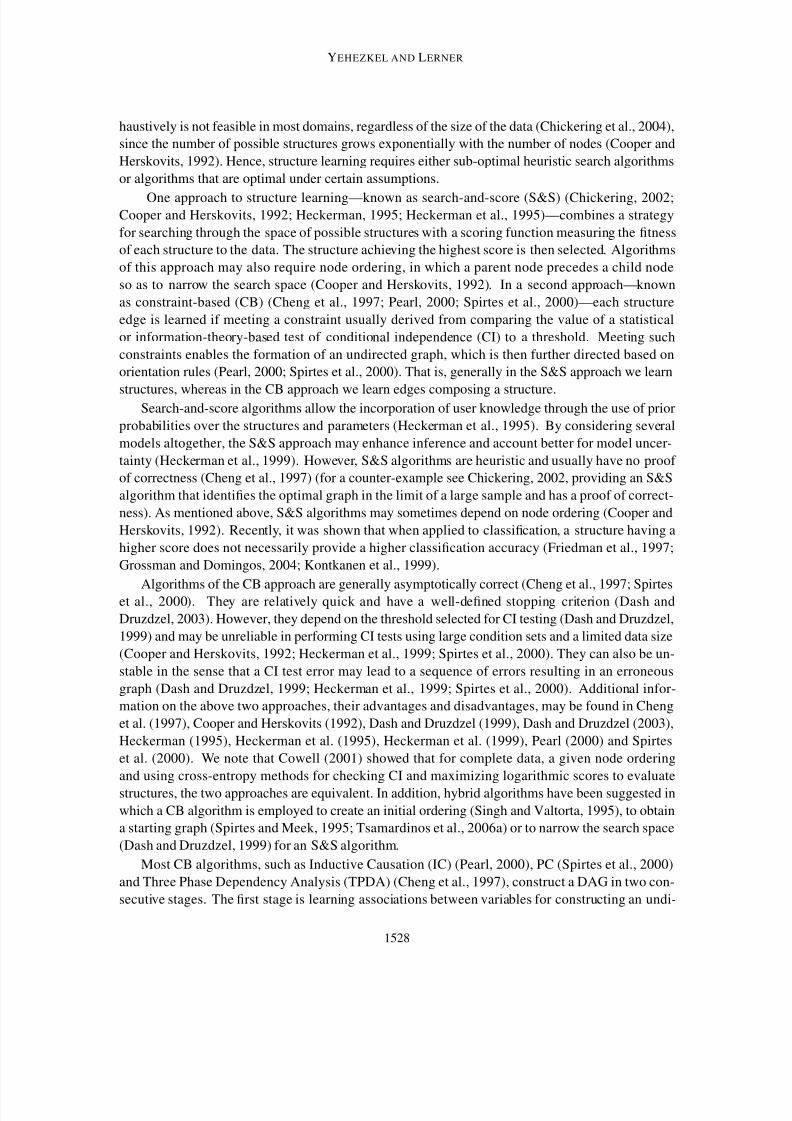
Definition 1 – d-separation resolution: The resolution of a d-separation relation between a pair of
non-adjacent nodes in a graph is the size of the smallest condition set that d-separates the two nodes.
Examples of d-separation resolutions of 0, 1 and 2 between nodes X and Y are given in Figure 1.
Definition 2 – d-separation resolution of a graph: The d-separation resolution of a graph is the
highest d-separation resolution in the graph.
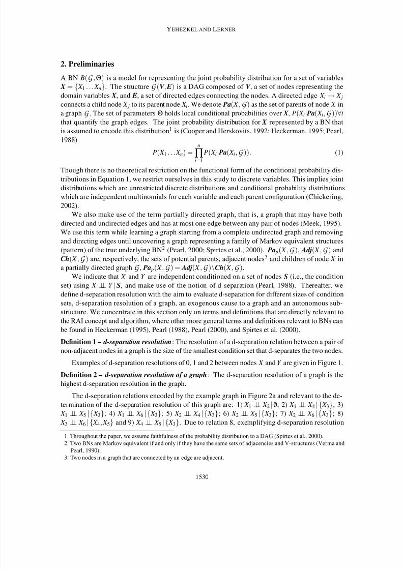
The d-separation relations encoded by the example graph in Figure 2a and relevant to the de-
termination of the d-separation resolution of this graph are: 1) X 1 ⊥⊥ X 2 | /0; 2) X 1 ⊥⊥ X 4 | { X 3}; 3)
X 1 ⊥⊥ X 5 | { X 3}; 4) X 1 ⊥⊥ X 6 | { X 3}; 5) X 2 ⊥⊥ X 4 | { X 3}; 6) X 2 ⊥⊥ X 5 | { X 3}; 7) X 2 ⊥⊥ X 6 | { X 3}; 8)
X 3 ⊥⊥ X 6 | { X 4, X 5} and 9) X 4 ⊥⊥ X 5 | { X 3}. Due to relation 8, exemplifying d-separation resolution
1. Throughout the paper, we assume faithfulness of the probability distribution to a DAG (Spirtes et al., 2000).
2. Two BNs are Markov equivalent if and only if they have the same sets of adjacencies and V-structures (Verma and
Pearl, 1990).
3. Two nodes in a graph that are connected by an edge are adjacent.
1530
8/3/2019 01-Bayesian Network Structure Learning by Recursive Autonomy Identification
http://slidepdf.com/reader/full/01-bayesian-network-structure-learning-by-recursive-autonomy-identification 5/44
BAYESIAN NETWORK STRUCTURE LEARNING BY RECURSIVE AUTONOMY IDENTIFICATION
X Y
Z X Y
ZX
Y
W Z
(a) (b) (c)
Figure 1: Examples of d-separation resolutions of (a) 0, (b) 1 and (c) 2 between nodes X and Y .
of 2, the d-separation resolution of the graph is 2. Eliminating relation 8 by adding the edge X 3 → X 6,
we form a graph having a d-separation resolution of 1 (Figure 2b). By further adding edges to the
graph, eliminating relations of resolution 1, we form a graph having a d-separation resolution of 0
(Figure 2c) that encodes only relation 1.
X X¡
X¢
X £ X ¤
X ¥
X¦
X§
X
X © X
X
X
X
X
X
X
X
(a) (b) (c)
Figure 2: Examples of graph d-separation resolutions of (a) 2, (b) 1 and (c) 0.
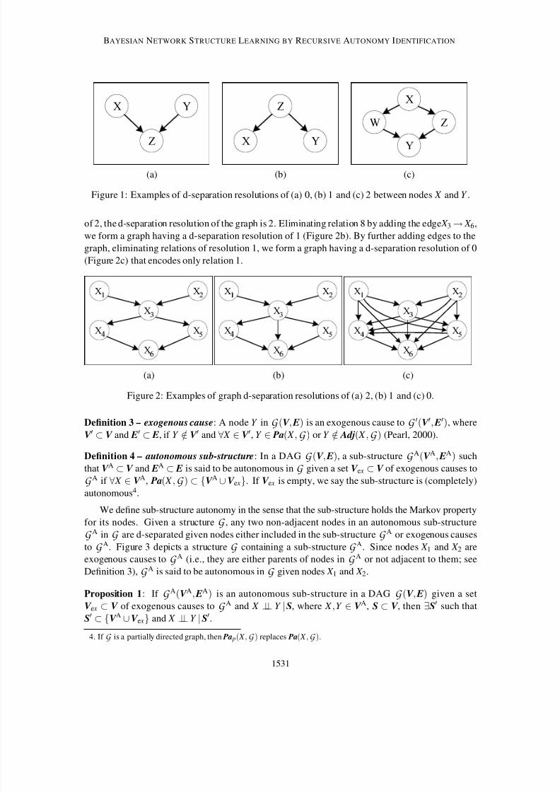
Definition 3 – exogenous cause: A node Y in G (V , E) is an exogenous cause to G ′(V ′, E′), where
V ′ ⊂ V and E′ ⊂ E, if Y /∈ V ′ and ∀ X ∈ V ′, Y ∈ Pa( X ,G ) or Y /∈ Adj( X ,G ) (Pearl, 2000).
Definition 4 – autonomous sub-structure: In a DAG G (V , E), a sub-structure G A(V A, EA) such
that V A ⊂ V and EA ⊂ E is said to be autonomous in G given a set V e x ⊂ V of exogenous causes to
G A if ∀ X ∈ V A, Pa( X ,G ) ⊂ {V A ∪ V e x}. If V e x is empty, we say the sub-structure is (completely)
autonomous4.
We define sub-structure autonomy in the sense that the sub-structure holds the Markov property
for its nodes. Given a structure G , any two non-adjacent nodes in an autonomous sub-structure
G A in G are d-separated given nodes either included in the sub-structure G A or exogenous causes
to G A. Figure 3 depicts a structure G containing a sub-structure G A. Since nodes X 1 and X 2 are
exogenous causes to G A (i.e., they are either parents of nodes in G A or not adjacent to them; see
Definition 3), G A is said to be autonomous in G given nodes X 1 and X 2.
Proposition 1: If G A(V A, EA) is an autonomous sub-structure in a DAG G (V , E) given a set
V e x ⊂ V of exogenous causes to G A and X ⊥⊥ Y | S, where X ,Y ∈ V A, S ⊂ V , then ∃S′ such that
S′ ⊂ {V A ∪ V e x} and X ⊥⊥ Y | S′.
4. If G is a partially directed graph, then Pa p( X ,G ) replaces Pa( X ,G ).
1531

8/3/2019 01-Bayesian Network Structure Learning by Recursive Autonomy Identification
http://slidepdf.com/reader/full/01-bayesian-network-structure-learning-by-recursive-autonomy-identification 6/44
YEHEZKEL AND LERNER
X X
X
X!
X"
G (V ;E )
G A(V A;E A)
Figure 3: An example of an autonomous sub-structure.
Proof : The proof is based on Lemma 1.
Lemma 1: If in a DAG, X and Y are non-adjacent and X is not a descendant of Y ,5 then X and Y
are d-separated given Pa(Y ) (Pearl, 1988; Spirtes et al., 2000).
If in a DAG G (V , E), X ⊥⊥ Y | S for some set S, where X and Y are non-adjacent, and if X is
not a descendant of Y , then, according to Lemma 1, X and Y are d-separated given Pa(Y ). Since X
and Y are contained in the sub-structure G A(V A, EA), which is autonomous given the set of nodes
V e x, then, following the definition of an autonomous sub-structure, all parents of the nodes in V A—
and specifically Pa(Y )—are members in set {V A ∪ V e x}. Then, ∃S′ such that S′ ⊂ {V A ∪ V e x} and
X ⊥⊥ Y | S′, which proves Proposition 1.
3. Recursive Autonomy Identification
Starting from a complete undirected graph and proceeding from low to high graph d-separation res-
olution, the RAI algorithm uncovers the correct pattern6 of a structure by performing the following
sequence of operations: (1) test of CI between nodes, followed by the removal of edges related
to independences, (2) edge direction according to orientation rules, and (3) graph decomposition
into autonomous sub-structures. For each autonomous sub-structure, the RAI algorithm is applied
recursively, while increasing the order of CI testing.
CI testing of order n between nodes X and Y is performed by thresholding the value of a criterion
that measures the dependence between the nodes conditioned on a set of n nodes (i.e., the condition
set) from the parents of X or Y . The set is determined by the Markov property (Pearl, 2000), for
example, if X is directed into Y , then only Y ’s parents are included in the set. Commonly, this
criterion is the χ2 goodness of fit test (Spirtes et al., 2000) or conditional mutual information (CMI)
(Cheng et al., 1997).
5. If X is a descendant of Y , we change the roles of X and Y and replace Pa(Y ) with Pa( X ).
6. In the absence of a topological node ordering, uncovering the correct pattern is the ultimate goal of BN structure
learning algorithms, since a pattern represents the same set of probabilities as that of the true structure (Spirtes et al.,
2000).
1532
8/3/2019 01-Bayesian Network Structure Learning by Recursive Autonomy Identification
http://slidepdf.com/reader/full/01-bayesian-network-structure-learning-by-recursive-autonomy-identification 7/44
BAYESIAN NETWORK STRUCTURE LEARNING BY RECURSIVE AUTONOMY IDENTIFICATION
Directing edges is conducted according to orientation rules (Pearl, 2000; Spirtes et al., 2000).
Given an undirected graph and a set of independences, both being the result of CI testing, the
following two steps are performed consecutively. First, intransitive triplets of nodes (V-structures)
are identified, and the corresponding edges are directed. An intransitive triplet X → Z ← Y is defined
if 1) X and Y are non-adjacent neighbors of Z , and 2) Z is not in the condition set that separated X and Y . In the second step, also known as the inductive stage, edges are continually directed until
no more edges can be directed, while assuring that no new V-structures and no directed cycles are
created.
Decomposition into separated, smaller, autonomous sub-structures reveals the structure hierar-
chy. Decomposition also decreases the number and length of paths between nodes that are CI-tested,
thereby diminishing, respectively, the number of CI tests and the sizes of condition sets used in these
tests. Both reduce computational complexity. Moreover, due to decomposition, additional edges can
be directed, which reduces the complexity of CI testing of the subsequent iterations. Following de-
composition, the RAI algorithm identifies ancestor and descendant sub-structures; the former are
autonomous, and the latter are autonomous given nodes of the former.
3.1 The RAI Algorithm
Similarly to other algorithms of structure learning (Cheng et al., 1997; Cooper and Herskovits, 1992;
Heckerman, 1995), the RAI algorithm7 assumes that all the independences entailed from the given
data can be encoded by a DAG. Similarly to other CB algorithms of structure learning (Cheng et al.,
1997; Spirtes et al., 2000), the RAI algorithm assumes that the data sample size is large enough for
reliable CI tests.
An iteration of the RAI algorithm starts with knowledge produced in the previous iteration and
the current d-separation resolution, n. Previous knowledge includes G start, a structure having a d-
separation resolution of n − 1, and G ex, a set of structures each having possible exogenous causes to
G start. Another input is the graph G all, which contains G start, G ex and edges connecting them. Note
that G all may also contain other nodes and edges, which may not be required for the learning task (e.g., edges directed from nodes in G start into nodes that are not in G start or G ex), and these will be
ignored by the RAI. In the first iteration, n = 0, G ex = /0, G start(V , E) is the complete undirected
graph and the d-separation resolution is not defined, since there are no pairs of d-separated nodes.
Since G ex is empty, G all = G start.
Given a structure G start having d-separation resolution n − 1, the RAI algorithm seeks indepen-
dences between adjacent nodes conditioned on sets of size n and removes the edges corresponding
to these independences. The resulting structure has a d-separation resolution of n. After applying
orientation rules so as to direct the remaining edges, a partial topological order is obtained in which
parent nodes precede their descendants. Childless nodes have the lowest topological order. This
order is partial, since not all the edges can be directed; thus, edges that cannot be directed connect
nodes of equal topological order. Using this partial topological ordering, the algorithm decomposesthe structure into ancestor and descendent autonomous sub-structures so as to reduce the complexity
of the successive stages.
First, descendant sub-structures are established containing the lowest topological order nodes. A
descendant sub-structure may be composed of a single childless node or several adjacent childless
7. The RAI algorithm and a preliminary experimental evaluation of the algorithm were introduced in Yehezkel and
Lerner (2005).
1533

8/3/2019 01-Bayesian Network Structure Learning by Recursive Autonomy Identification
http://slidepdf.com/reader/full/01-bayesian-network-structure-learning-by-recursive-autonomy-identification 8/44
YEHEZKEL AND LERNER
nodes. We will further refer to a single descendent sub-structure, although such a sub-structure
may consist of several non-connected sub-structures. Second, all edges pointing towards nodes of
the descendant sub-structure are temporarily removed (together with the descendant sub-structure
itself), and the remaining clusters of connected nodes are identified as ancestor sub-structures. The
descendent sub-structure is autonomous, given nodes of higher topological order composing theancestor sub-structures. To consider smaller numbers of parents (and thereby smaller condition set
sizes) when CI testing nodes of the descendant sub-structure, the algorithm first learns ancestor
sub-structures, then the connections between ancestor and descendant sub-structures, and finally
the descendant sub-structure itself. Each ancestor or descendent sub-structure is further learned
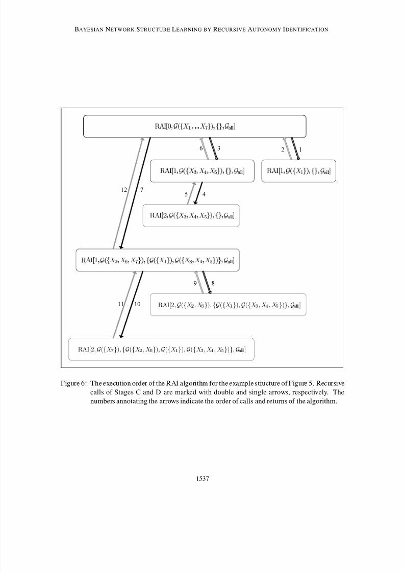
by recursive calls to the algorithm. Figures 4, 5 and 6 show, respectively, the RAI algorithm, a
manifesting example and the algorithm execution order for this example.
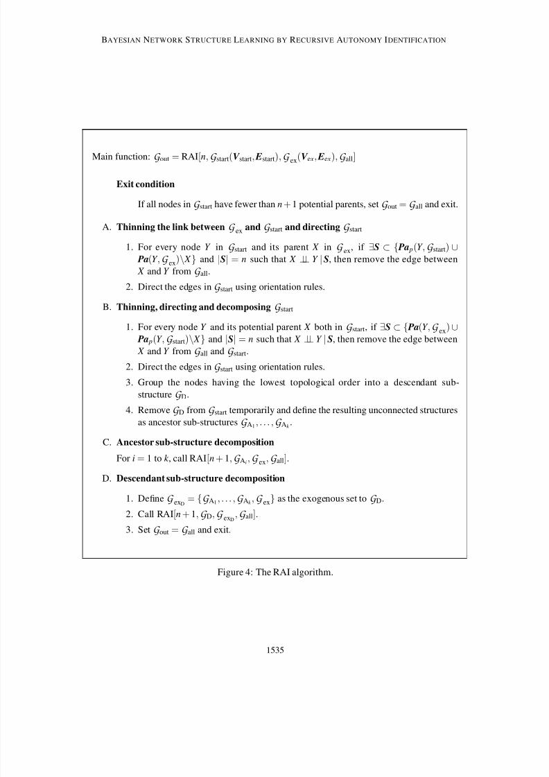
The RAI algorithm is composed of four stages (denoted in Figure 4 as Stages A, B, C and
D) and an exit condition checked before the execution of any of the stages. The purpose of the
exit condition is to assure that a CI test of a required order can indeed be performed, that is, the
number of potential parents required to perform the test is adequate. The purpose of Stage A1 is
to thin the link between G ex and G start, the latter having d-separation resolution of n − 1. This isachieved by removing edges corresponding to independences between nodes in G ex and nodes in
G start conditioned on sets of size n of nodes that are either exogenous to, or within, G start. Similarly,
in Stage B1, the algorithm tests for CI of order n between nodes in G start given sets of size n of nodes
that are either exogenous to, or within, G start, and removes edges corresponding to independences.
The edges removed in Stages A1 and B1 could not have been removed in previous applications of
these stages using condition sets of lower orders. When testing independence between X and Y ,
conditioned on the potential parents of node X , those nodes in the condition set that are exogenous
to G start are X ’s parents whereas those nodes that are in G start are either its parents or adjacents.
In Stages A2 and B2, the algorithm directs every edge from the remaining edges that can be
directed. In Stage B3, the algorithm groups in a descendant sub-structure all the nodes having the
lowest topological order in the derived partially directed structure, and following the temporary re-moval of these nodes, it defines in Stage B4 separate ancestor sub-structures. Due to the topological
order, every edge from a node X in an ancestor sub-structure to a node Z in the descendant sub-
structure is directed as X → Z . In addition, there is no edge connecting one ancestor sub-structure
to another ancestor sub-structure.
Thus, every ancestor sub-structure contains all the potential parents of its nodes, that is, it is au-
tonomous (or if some potential parents are exogenous, then the sub-structure is autonomous given
the set of exogenous nodes). The descendant sub-structure is, by definition, autonomous given
nodes of ancestor sub-structures. Proposition 1 showed that we can identify all the conditional in-
dependences between nodes of an autonomous sub-structure. Hence, every ancestor and descendant
sub-structure can be processed independently in Stages C and D, respectively, so as to identify con-
ditional independences of increasing orders in each recursive call of the algorithm. Stage C is a
recursive call for the RAI algorithm for learning each ancestor sub-structure with order n + 1. Sim-
ilarly, Stage D is a recursive call for the RAI algorithm for learning the descendant sub-structure
with order n + 1, while assuming that the ancestor sub-structures have been fully learned (having
d-separation resolution of n + 1).
Figure 5 and Figure 6, respectively, show diagrammatically the stages in learning an example
graph and the execution order of the algorithm for this example. Figure 5a shows the true structure
that we wish to uncover. Initially, G start is the complete undirected graph (Figure 5b), n = 0, G ex is
1534
8/3/2019 01-Bayesian Network Structure Learning by Recursive Autonomy Identification
http://slidepdf.com/reader/full/01-bayesian-network-structure-learning-by-recursive-autonomy-identification 9/44
BAYESIAN NETWORK STRUCTURE LEARNING BY RECURSIVE AUTONOMY IDENTIFICATION
Main function: G out = RAI[n,G start(V start, Estart),G ex(V e x, Ee x),G all]
Exit condition
If all nodes in G start have fewer than n + 1 potential parents, set G out = G all and exit.
A. Thinning the link between G ex and G start and directing G start
1. For every node Y in G start and its parent X in G ex, if ∃S ⊂ { Pa p(Y ,G start) ∪ Pa(Y ,G ex)\ X } and |S| = n such that X ⊥⊥ Y | S, then remove the edge between
X and Y from G all.2. Direct the edges in G start using orientation rules.
B. Thinning, directing and decomposing G start
1. For every node Y and its potential parent X both in G start, if ∃S ⊂ { Pa(Y ,G ex) ∪ Pa p(Y ,G start)\ X } and |S| = n such that X ⊥⊥ Y | S, then remove the edge between
X and Y from G all and G start.
2. Direct the edges in G start using orientation rules.
3. Group the nodes having the lowest topological order into a descendant sub-
structure G D.
4. Remove G D from G start temporarily and define the resulting unconnected structuresas ancestor sub-structures G A1
, . . . ,G Ak .
C. Ancestor sub-structure decomposition
For i = 1 to k , call RAI[n + 1,G Ai,G ex,G all].
D. Descendant sub-structure decomposition
1. Define G exD= {G A1
, . . . ,G Ak ,G ex} as the exogenous set to G D.
2. Call RAI[n + 1,G D,G exD,G all].
3. Set G out = G all and exit.
Figure 4: The RAI algorithm.
1535

8/3/2019 01-Bayesian Network Structure Learning by Recursive Autonomy Identification
http://slidepdf.com/reader/full/01-bayesian-network-structure-learning-by-recursive-autonomy-identification 10/44
YEHEZKEL AND LERNER
X1
X2
X3
X4
X5
X6
X7
X1
X2
X3
X6
X7
X4
X5
X1
X2
X3
X6
X7
X4
X5
(a) (b) (c)
X1
X2
X3
X6
X7
X4
X5
X1
X2
X3
X6
X7
G A # G A $
G D
X4
X5
X3
X4
X5
(d) (e) (f)
% &
% '
% (
% ) % 0
% 1
% 2
3 4
3 5
3 6
3 7 3 8
3 9
3 @
X1
X2
X3
X4
X5
X6
X7
(g) (h) (i)
Figure 5: Learning an example structure. a) The true structure to learn, b) initial (complete) struc-
ture and structures learned by the RAI algorithm in Stages (see Figure 4) c) B1, d) B2,
e) B3 and B4, f) C, g) D and A1, h) D and A2 and i) D, B1 and B2 (i.e., the resulting
structure).
1536
8/3/2019 01-Bayesian Network Structure Learning by Recursive Autonomy Identification
http://slidepdf.com/reader/full/01-bayesian-network-structure-learning-by-recursive-autonomy-identification 11/44
BAYESIAN NETWORK STRUCTURE LEARNING BY RECURSIVE AUTONOMY IDENTIFICATION
A
B C D
E F G H
I
P Q R R R P S T
U
F
I
T F G
V W W X
Y
a b
c
d e f
g
h i p
q
d
g
p
d e
r s s t
u
v
w x
y
� � �
�
� �
�
� �
�
� � �
�
�
�
�
� �
� � � �
�
� � �
� � �
�
�
j
k
�
j
� �
l m m n
o
z
{ |
}
~ |
}
|
}
|
RAI[2; G (fX
; X g); fG (fX
g); G (fX
; X ; X
� g)g; G � � � ]
RAI[2;G (fX � g);fG (fX
� ; X
� g);G (fX
g); G (fX ; X ; X g)g;G
]
457
89
1011
12
1236
Figure 6: The execution order of the RAI algorithm for the example structure of Figure 5. Recursive
calls of Stages C and D are marked with double and single arrows, respectively. The
numbers annotating the arrows indicate the order of calls and returns of the algorithm.
1537

8/3/2019 01-Bayesian Network Structure Learning by Recursive Autonomy Identification
http://slidepdf.com/reader/full/01-bayesian-network-structure-learning-by-recursive-autonomy-identification 12/44
YEHEZKEL AND LERNER
empty and G all = G start, so Stage A is skipped. In Stage B1, any pair of nodes in G start is CI tested
given an empty condition set (i.e., checking marginal independence), which yields the removal of the
edges between node X 1 and nodes X 3, X 4 and X 5 (Figure 5c). The edge directions inferred in Stage
B2 are shown in Figure 5d. The nodes having the lowest topological order ( X 2, X 6, X 7) are grouped
into a descendant sub-structure G D (Stage B3), while the remaining nodes form two unconnectedancestor sub-structures, G A1
and G A2(Stage B4)(Figure 5e). Note that after decomposition, every
edge between a node, X i, in an ancestor sub-structure, and a node, X j, in a descendant sub-structure
is a directed edge X i → X j. The set of all edges from an ancestor sub-structure to the descendant
sub-structure is illustrated in Figure 5e by a wide arrow connecting the sub-structures. In Stage C,
the algorithm is called recursively for each of the ancestor sub-structures with n = 1, G start = G Ai
(i = 1,2) and G ex = /0. Since sub-structure G A1contains a single node, the exit condition for this
structure is satisfied. While calling G start = G A2, Stage A is skipped, and in Stage B1 the algorithm
identifies that X 4 ⊥⊥ X 5 | X 3, thus removing the edge X 4 – X 5. No orientations are identified (e.g., X 3cannot be a collider, since it separated X 4 and X 5), so the three nodes have equal topological order
and they are grouped to form a descendant sub-structure. The recursive call for this sub-structure
with n = 2 is returned immediately, since the exit condition is satisfied (Figure 5f). Moving toStage D, the RAI is called with n = 1, G start = G D and G ex = {G A1
,G A2}. Then, in Stage A1
relations X 1 ⊥⊥ { X 6, X 7} | X 2, X 4 ⊥⊥ { X 6, X 7} | X 2 and { X 3, X 5} ⊥⊥ { X 2, X 6, X 7} | X 4 are identified, and
the corresponding edges are removed (Figure 5g). In Stage A2, X 6 and X 7 cannot collide at X 2(since X 6 and X 7 are adjacent), and X 2 and X 6 ( X 7) cannot collide at X 7 ( X 6) (since X 2 and X 6 ( X 7)
are adjacent); hence, no additional V-structures are formed. Based on the inductive step and since
X 1 is directed at X 2, X 2 should be directed at X 6 and at X 7. X 6 ( X 7) cannot be directed at X 7 ( X 6),
because no new V-structures are allowed (Figure 5h). Stage B1 of the algorithm identifies the
relation X 2 ⊥⊥ X 7 | X 6 and removes the edge X 2 → X 7. In Stage B2, X 6 cannot be a collider of X 2and X 7, since it has separated them. In the inductive step, X 6 is directed at X 7, X 6 → X 7 (Figure 5i).
In Stages B3 and B4, X 7 and { X 2, X 6} are identified as a descendant sub-structure and an ancestor
sub-structure, respectively. Further recursive calls (8 and 10 in Figure 6) are returned immediately,
and the resulting partially directed structure (Figure 5i) represents a family of Markov equivalent
structures (pattern) of the true structure (Figure 5a).
3.2 Minimality, Stability and Complexity
After describing the RAI algorithm (Section 3.1) and before proving its correctness (Section 3.3), we
analyze in Section 3.2 three essential aspects of the algorithm—minimality, stability and complexity.
3.2.1 MINIMALITY
A structure recovered by the RAI algorithm in iteration m has a higher d-separation resolution and
entails fewer dependences and thus is simpler and preferred 8 to a structure recovered in iteration
m − k where 0 < k ≤ m. By increasing the resolution, the RAI algorithm, similarly to the PCalgorithm, moves from a complete undirected graph having maximal dependence relations between
variables to structures having less (or equal) dependences than previous structures, ending in a
structure having no edges between conditionally independent nodes, that is, a minimal structure.
8. We refer here to structures learned during algorithm execution and do not consider the empty graph that naturally has
the lowest d-separation resolution (i.e., 0). This graph, having all nodes marginally independent of each other, will
be found by the RAI algorithm immediately after the first iteration for graph resolution 0.
1538
8/3/2019 01-Bayesian Network Structure Learning by Recursive Autonomy Identification
http://slidepdf.com/reader/full/01-bayesian-network-structure-learning-by-recursive-autonomy-identification 13/44
BAYESIAN NETWORK STRUCTURE LEARNING BY RECURSIVE AUTONOMY IDENTIFICATION
3.2.2 STABILITY
Similarly to Spirtes et al. (2000), we use the notion of stability informally to measure the number of
errors in the output of a stage of the algorithm due to errors in the input to this stage. Similarly to the
PC algorithm, the main sources of errors of the RAI algorithm are CI-testing and the identificationof V-structures. Removal of an edge due to an erroneous CI test may lead to failure in correctly
removing other edges, which are not in the true graph and also cause to orientation errors. Failure
to remove an edge due to an erroneous CI test may prevent, or wrongly cause, orientation of edges.
Missing or wrongly identifying a V-structure affect the orientation of other edges in the graph during
the inductive stage and subsequent stages.
Many CI test errors (i.e., deciding that (in)dependence exists where it does not) in CB algo-
rithms are the result of unnecessary large condition sets given a limited database size (Spirtes et al.,
2000). Large condition sets are more likely to be inaccurate, since they are more likely to include
unnecessary and erroneous nodes (erroneous due to errors in earlier stages of the algorithm). These
sets may also cause poorer estimation of the criterion that measures dependence (e.g., CMI or χ2)
due to the curse-of-dimensionality, as typically there are only too few instances representing some
of the combinations of node states. Either way, these condition sets are responsible for many wrong
decisions about whether dependence between two nodes exists or not. Consequently, these errors
cause structural inaccuracies and hence also poor inference ability.
Although CI-testing in the PC algorithm is more stable than V-structure identification (Spirtes
et al., 2000), it is difficult to say whether this is also the case in the RAI algorithm. Being recursive,
the RAI algorithm might be more unstable. However, CI test errors are practically less likely to
occur, since by alternating between CI testing and edge direction the algorithm uses knowledge
about parent-child relations before CI testing of higher orders. This knowledge permits avoiding
some of the tests and decreases the size of conditions sets of some other tests (see Lemma 1). In
addition, graph decomposition promotes decisions about well-founded orders of node presentation
for subsequent CI tests, contrary to the common arbitrary order of presentation (see, e.g., the PC
algorithm). Both mechanisms enhance stability and provide some means of error correction, as will
be demonstrated shortly.
Let us now extensively describe examples that support our claim regarding the enhanced sta-
bility of the RAI algorithm. Suppose that following CI tests of some order both the PC and RAI
algorithms identify a triplet of nodes in which two non-adjacent nodes, X and Y , are adjacent to a
third node, Z , that is, X – Z – Y . In the immediate edge direction stage, the RAI algorithm identifies
this triplet as a V-structure, X → Z ← Y . Now, suppose that due to an unreliable CI test of a higher
order the PC algorithm removes X – Z and the RAI algorithm removes X → Z . Eventually, both
algorithms fail to identify the V-structure, but the RAI algorithm has an advantage over the PC algo-
rithm in that the other arm of the V-structure is directed, Z ← Y . This contributes to the possibility to
direct further edges during the inductive stage and subsequent recursive calls for the algorithm. The
directed arm would also contribute to fewer CI tests and tests with smaller condition sets during CI
testing with higher orders (e.g., if we later have to test independence between Y and another node,
then we know that Z should not be included in the condition set, even though it is adjacent to Y ). In
addition, the direction of this edge also contributes to enhanced inference capability.
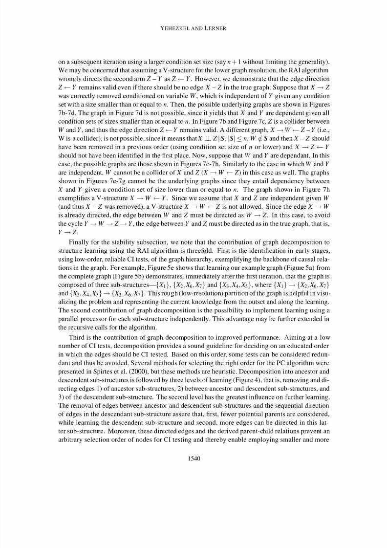
Now, suppose another example in which after removing all edges due to reliable CI tests using
condition set sizes lower than or equal to n, the algorithm identifies the V-structure X → Z ← Y
(Figure 7a). However, let assume that one of the V-structure arms, say X → Z , is correctly removed
1539
8/3/2019 01-Bayesian Network Structure Learning by Recursive Autonomy Identification
http://slidepdf.com/reader/full/01-bayesian-network-structure-learning-by-recursive-autonomy-identification 14/44
YEHEZKEL AND LERNER
on a subsequent iteration using a larger condition set size (say n + 1 without limiting the generality).
We may be concerned that assuming a V-structure for the lower graph resolution, the RAI algorithm
wrongly directs the second arm Z – Y as Z ← Y . However, we demonstrate that the edge direction
Z ← Y remains valid even if there should be no edge X – Z in the true graph. Suppose that X → Z
was correctly removed conditioned on variable W , which is independent of Y given any conditionset with a size smaller than or equal to n. Then, the possible underlying graphs are shown in Figures
7b-7d. The graph in Figure 7d is not possible, since it yields that X and Y are dependent given all
condition sets of sizes smaller than or equal to n. In Figure 7b and Figure 7c, Z is a collider between
W and Y , and thus the edge direction Z ← Y remains valid. A different graph, X → W ← Z – Y (i.e.,
W is a collider), is not possible, since it means that X ⊥⊥ Z | S, |S| ≤ n, W /∈ S and then X – Z should
have been removed in a previous order (using condition set size of n or lower) and X → Z ← Y
should not have been identified in the first place. Now, suppose that W and Y are dependant. In this
case, the possible graphs are those shown in Figures 7e-7h. Similarly to the case in which W and Y
are independent, W cannot be a collider of X and Z ( X → W ← Z ) in this case as well. The graphs
shown in Figures 7e-7g cannot be the underlying graphs since they entail dependency between
X and Y given a condition set of size lower than or equal to n. The graph shown in Figure 7hexemplifies a V-structure X → W ← Y . Since we assume that X and Z are independent given W
(and thus X – Z was removed), a V-structure X → W ← Z is not allowed. Since the edge X → W
is already directed, the edge between W and Z must be directed as W → Z . In this case, to avoid
the cycle Y → W → Z → Y , the edge between Y and Z must be directed as in the true graph, that is,
Y → Z .
Finally for the stability subsection, we note that the contribution of graph decomposition to
structure learning using the RAI algorithm is threefold. First is the identification in early stages,
using low-order, reliable CI tests, of the graph hierarchy, exemplifying the backbone of causal rela-
tions in the graph. For example, Figure 5e shows that learning our example graph (Figure 5a) from
the complete graph (Figure 5b) demonstrates, immediately after the first iteration, that the graph is
composed of three sub-structures—{ X 1}, { X 2, X 6, X 7} and { X 3, X 4, X 5}, where { X 1} → { X 2, X 6, X 7}and { X 3, X 4, X 5} → { X 2, X 6, X 7}. This rough (low-resolution) partition of the graph is helpful in visu-
alizing the problem and representing the current knowledge from the outset and along the learning.
The second contribution of graph decomposition is the possibility to implement learning using a
parallel processor for each sub-structure independently. This advantage may be further extended in
the recursive calls for the algorithm.
Third is the contribution of graph decomposition to improved performance. Aiming at a low
number of CI tests, decomposition provides a sound guideline for deciding on an educated order
in which the edges should be CI tested. Based on this order, some tests can be considered redun-
dant and thus be avoided. Several methods for selecting the right order for the PC algorithm were
presented in Spirtes et al. (2000), but these methods are heuristic. Decomposition into ancestor and
descendent sub-structures is followed by three levels of learning (Figure 4), that is, removing and di-
recting edges 1) of ancestor sub-structures, 2) between ancestor and descendent sub-structures, and
3) of the descendent sub-structure. The second level has the greatest influence on further learning.
The removal of edges between ancestor and descendent sub-structures and the sequential direction
of edges in the descendant sub-structure assure that, first, fewer potential parents are considered,
while learning the descendent sub-structure and second, more edges can be directed in this lat-
ter sub-structure. Moreover, these directed edges and the derived parent-child relations prevent an
arbitrary selection order of nodes for CI testing and thereby enable employing smaller and more
1540

8/3/2019 01-Bayesian Network Structure Learning by Recursive Autonomy Identification
http://slidepdf.com/reader/full/01-bayesian-network-structure-learning-by-recursive-autonomy-identification 15/44
BAYESIAN NETWORK STRUCTURE LEARNING BY RECURSIVE AUTONOMY IDENTIFICATION
X Y
Z
X Y
ZW
X Y
ZW
(a) (b) (c)
X Y
Z
W
X Y
Z
W
X Y
Z
W
(d) (e) (f)
X Y
Z
W
X Y
Z
W
(g) (h)
Figure 7: Graphs used to exemplify the stability of the RAI algorithm (see text).
accurate condition sets. Take, for example, CI testing for the redundant edge between X 2 and X 7in our example graph (Figure 5i) if the RAI algorithm did not use decomposition. Graph decom-
position for n = 0 (Figure 5e) enables the identification of two ancestor sub-structures, G A1and
G A2, as well as a descendent sub-structure G D that are each learned recursively. During Stage D
(Figure 4) and while thinning the links between the ancestor sub-structures and G D (in Stage A1
of the recursion for n = 1), we identify the relations X 1 ⊥⊥ { X 6, X 7} | X 2, X 4 ⊥⊥ { X 6, X 7} | X 2 and
{ X 3, X 5} ⊥⊥ { X 2, X 6, X 7} | X 4 and remove the 10 corresponding edges (Figure 5g). The decision to
test and remove these edges first was enabled by the decomposition of the graph to G A1, G A2
and
G D
. In Stage A2 (Figure 5h), we direct the edge X 2
→ X 6
(as X 1
⊥⊥ X 6
| X 2
and thus X 2
cannot be
a collider between X 1 and X 6) and edge X 2 → X 7 (as X 1 ⊥⊥ X 7 | X 2 and thus X 2 cannot be a collider
between X 1 and X 7), and in Stage B (Figure 5i) we direct the edge X 6 → X 7. The direction of these
edges could not be assured without removing first the above edges, since the (redundant) edges
pointing onto X 6 and X 7 would have allowed wrong edge direction, that is, X 6 → X 2 and X 7 → X 2.
If we had been using the RAI algorithm with no decomposition (Figure 5d) (or the PC algorithm)
and had decided to check the independence between X 2 and X 7, first, we would have had to consider
condition sets containing the nodes X 1, X 3, X 4, X 5 or X 6 (up to 10 CI tests whether we start from
1541
8/3/2019 01-Bayesian Network Structure Learning by Recursive Autonomy Identification
http://slidepdf.com/reader/full/01-bayesian-network-structure-learning-by-recursive-autonomy-identification 16/44
YEHEZKEL AND LERNER
X 2 or X 7). Instead, we perform in Stage B1 only one test, X 2 ⊥⊥ X 7 | X 6. These benefits are the result
of graph decomposition.
3.2.3 COMPLEXITY
CI tests are the major contributors to the (run-time) complexity of CB algorithms (Cheng and
Greiner, 1999). In the worst case, the RAI algorithm will neither direct any edges nor decom-
pose the structure and will thus identify the entire structure as a descendant sub-structure, calling
Stages D and B1 iteratively while skipping all other stages. Then, the execution of the algorithm
will be similar to that of the PC algorithm, and thus the complexity will be bounded by that of the
PC algorithm. Given the maximal number of possible parents k and the number of nodes n, the
number of CI tests is bounded by (Spirtes et al., 2000)
2
n
2
·
k
∑i=0
n − 1
i
≤
n2(n − 1)k −1
(k − 1)!,
which leads to complexity of O(nk ).This bound is loose even in the worst case (Spirtes et al., 2000) especially in real-world ap-
plications requiring graphs having V-structures. This means that in most cases some edges are
directed and the structure is decomposed; hence, the number of CI tests is much smaller than that
of the worst case. For example, by decomposing our example graph (Figure 5) into descendent
and ancestor sub-structures in the first application of Stage B4 (Figure 5e), we avoid checking
X 6 ⊥⊥ X 7 | { X 1, X 3, X 4, X 5}. This is because { X 1, X 3, X 4, X 5} are neither X 6’s nor X 7’s parents and thus
are not included in the (autonomous) descendent sub-structure. By checking only X 6 ⊥⊥ X 7 | { X 2},
the RAI algorithm saves CI tests that are performed by the PC algorithm. We will further elaborate
on the RAI algorithm complexity in our forthcoming study.
3.3 Proof of Correctness
We prove the correctness of the RAI algorithm using Proposition 2. We show that only conditional
independences (of all orders) entailed by the true underlying graph are identified by the RAI al-
gorithm and that all V-structures are correctly identified. We then note on the correctness of edge
direction.
Proposition 2: If the input data to the RAI algorithm are faithful to a DAG, G true, having any
d-separation resolution, then the algorithm yields the correct pattern for G true.
Proof : We use mathematical induction to prove the proposition, where in each induction step, m,
we prove that the RAI algorithm finds (a) all conditional independences of order m and lower, (b)
no false conditional independences, (c) only correct V-structures and (d) all V-structures, that is, noV-structures are missing.
Base step (m = 0): If the input data to the RAI algorithm was generated from a distribution faithful
to a DAG, G true, having d-separation resolution 0, then the algorithm yields the correct pattern for
G true.
Given that the true underlying DAG has a d-separation resolution of 0, the data entail only
marginal independences. In the beginning of learning, G start is a complete graph and m = 0. Since
1542
8/3/2019 01-Bayesian Network Structure Learning by Recursive Autonomy Identification
http://slidepdf.com/reader/full/01-bayesian-network-structure-learning-by-recursive-autonomy-identification 17/44
BAYESIAN NETWORK STRUCTURE LEARNING BY RECURSIVE AUTONOMY IDENTIFICATION
there are no exogenous causes, Stage A is skipped. In Stage B, the algorithm tests for independence
between every pair of nodes with an empty condition set, that is, X ⊥⊥ Y | /0 (marginal independence),
removes the redundant edges and directs the remaining edges as possible. In the resulting structure,
all the edges between independent nodes have been removed and no false conditional independences
are entailed. Thus, all the identified V-structures are correct, as discussed in Section 3.2.2 on stabil-ity, and there are no missing V-structures, since the RAI algorithm has tested independence for all
pair of nodes (edges). At the end of Stage B2 (edge direction), the resulting structure and G true have
the same set of V-structures and the same set of edges. Thus, the correct pattern for G true is identi-
fied. Since the data entail only independences of zero order, further recursive calls with m ≥ 1 will
not find independences with condition sets of size m, and thus no edges will be removed, leaving
the graph unchanged.
Inductive step (m + 1): Suppose that at induction step m, the RAI algorithm discovers all condi-
tional independences of order m and lower, no false conditional independences are entailed, all
V-structures are correct, and no V-structures are missing. Then, if the input data to the RAI al-
gorithm was generated from a distribution faithful to a DAG, G true, having d-separation resolutionm + 1, then the RAI algorithm would yield the correct pattern for that graph.
In step m, the RAI algorithm discovers all conditional independences of order m and lower.
Given input data faithful to a DAG, G true, having d-separation resolution m + 1, there exists at
least one pair of nodes, say { X ,Y }, in the true graph, that has a d-separation resolution of m + 1.9
Since the RAI, by the recursive call m + 1 (i.e., calling RAI[m + 1,G start,G ex,G all]), has identified
only conditional independences of order m and lower, an edge, E XY = ( X – Y ), exists in the input
graph, G start. The smallest condition set required to identify the independence between X and Y is
S XY ( X ⊥⊥ Y | S XY ), such that |S XY | ≥ m + 1. Thus, | Pa p( X )\Y | ≥ m + 1 or | Pa p(Y )\ X | ≥ m + 1,
meaning that either node X or node Y has at least m + 2 potential parents. Such an edge exists
in at least one of the autonomous sub-structures decomposed from the graph yielded at the end of
iteration m. When calling, in Stage C or Stage D, the algorithm recursively for this sub-structurewith m′ = m +1, the exit condition is not satisfied because either node X or node Y has at least m′ +1
parents. Since Step m assured that the sub-structure is autonomous, it contains all the necessary node
parents. Note that decomposition into ancestor, G A, and descendant, G D, sub-structures occurs after
identification of all nodes having the lowest topological order, such that every edge from a node
X in G A to a node Y in G D is directed, X → Y . In the case that the sub-structure is an ancestor
sub-structure, S XY contains nodes of the sub-structure and its exogenous causes. In the case that the
sub-structure is a descendant sub-structure, S XY contains nodes from the ancestor sub-structures and
the descendant sub-structure. Therefore, based on Proposition 1, the RAI algorithm tests all edges
using condition sets of sizes m′ and removes E XY (and all similar edges) in either Stage A or Stage
B, yielding a structure with d-separation resolution of m′ and thereby yields the correct pattern for
the true underlying graph of d-separation resolution m + 1.
Spirtes (2001)—when introducing the anytime fast casual inference (AFCI) algorithm—proved
the correctness of edge direction of AFCI. The AFCI algorithm can be interrupted at any stage
(resolution), and the resultant graph at this stage is correct with probability one in the large sample
9. If the d-separation resolution of { X ,Y } is m′ > m + 1, then the RAI algorithm will not modify the graph until step m′.
1543
8/3/2019 01-Bayesian Network Structure Learning by Recursive Autonomy Identification
http://slidepdf.com/reader/full/01-bayesian-network-structure-learning-by-recursive-autonomy-identification 18/44
YEHEZKEL AND LERNER
limit, although possibly less informative10 than if had been allowed to continue uninterrupted.11
Recall that interrupting learning means that we avoid CI tests of higher orders. This renders the
resultant graph more reliable. We use this proof here for proving the correctness of edge direction
in the RAI algorithm. Completing CI testing with a specific graph resolution n in the RAI algorithm
and interrupting the AFCI at any stage of CI testing are analogous. Furthermore, Spirtes (2001)proves that interrupting the algorithm at any stage is also possible during edge direction, that is,
once an edge is directed, the algorithm never changes that direction. In Section 3.2.2, we showed
that even if a directed edge of a V-structure is removed, the direction of the remaining edge is still
correct. Since directing edges by the AFCI algorithm after interruption yields a correct (although
less informative) graph (Spirtes, 2001), also the direction of edges by the RAI algorithm yields
a correct graph. Having (real) parents in a condition set used for CI testing, instead of potential
parents, which are the result of edge direction for resolutions lower than n, is a virtue, as was
confirmed in Section 3.1. All that is required that all parents, either real or potential, be included
within the corresponding condition set, and this is indeed guaranteed by the autonomy of each sub-
structure, as was proved above.
4. Experiments and Results
We compare the RAI algorithm with other state-of-the-art algorithms with respect to structural cor-
rectness, computational complexity, run-time and classification accuracy when the learned structure
is used in classification. The algorithms learned structures from databases representing synthetic
problems, real decision support systems and natural classification problems. We present the experi-
mental evaluation in four sections. In Section 4.1, the complexity of the RAI algorithm is measured
by the number of CI tests required for learning synthetically generated structures in comparison to
the complexity of the PC algorithm (Spirtes et al., 2000).
The order of presentation of nodes is not an input to the PC algorithm. Nevertheless, CI testing
of orders higher than 0, and therefore also edge directing, which depends on CI testing, may besensitive to that order. This may cause learning different graphs whenever the order is changed.
Dash and Druzdzel (1999) turned this vice of the PC algorithm into a virtue by employing the
partially directed graphs formed by using different orderings for the PC algorithm as the search
space from which the structure having the highest value of the K2 metric (Cooper and Herskovits,
1992) is selected. For the RAI algorithm, sensitivity to the order of presentation of nodes is expected
to be reduced compared to the PC algorithm, since the RAI algorithm, due to edge direction and
graph decomposition, decides on the order of performing most of the CI tests and does not use an
arbitrary order (Section 3.2.2). Nevertheless, to account for the possible sensitivity of the RAI and
PC algorithms to this order, we preliminarily employed 100 different permutations 12 of the order for
each of ten Alarm network (Beinlich et al., 1989) databases. Since the results of these experiments
10. Less informative in the sense that it answers “can’t tell” for a larger number of questions; that is, identifying, for
example, “◦” edge endpoint (placing no restriction on the relation between the pair of nodes making the edge) instead
of “→” endpoint.
11. The AFCI algorithm is also correct if hidden and selection variables exist. A selection variable models the possibility
of an observable variable having some missing data. We focus here on the case where neither hidden nor selection
variables exist.
12. Dash and Druzdzel (1999) examined the relationships between the number of order permutations and the numbers of
variables and instances. We fixed the number of order permutations at 100.
1544
8/3/2019 01-Bayesian Network Structure Learning by Recursive Autonomy Identification
http://slidepdf.com/reader/full/01-bayesian-network-structure-learning-by-recursive-autonomy-identification 19/44
BAYESIAN NETWORK STRUCTURE LEARNING BY RECURSIVE AUTONOMY IDENTIFICATION
had showed that the difference in performance for different permutations is slight, we further limited
the experiments with the PC and RAI algorithms to a single permutation.
In Section 4.2, we present our methodology of selecting a threshold for RAI CI testing. We
propose selecting a threshold for which the learned structure has a maximum of a likelihood-based
score value.In Section 4.3, we use the Alarm network (Beinlich et al., 1989), which is a widely accepted
benchmark for structure learning, to evaluate the structural correctness of graphs learned by the
RAI algorithm. The correctness of the structure recovered by RAI is compared to those of struc-
tures learned using other algorithms—PC, TPDA (Cheng et al., 1997), GES (Chickering, 2002;
Meek, 1997), SC (Friedman et al., 1999) and MMHC (Tsamardinos et al., 2006a). The PC and
TPDA algorithms are the most popular CB algorithms (Cheng et al., 2002; Kennett et al., 2001;
Marengoni et al., 1999; Spirtes et al., 2000); GES and SC are state-of-the-art S&S algorithms
(Tsamardinos et al., 2006a); and MMHC is a hybrid algorithm that has recently been developed and
showed superiority, with respect to different criteria, over all the (non-RAI) algorithms examined
here (Tsamardinos et al., 2006a). In addition to correctness, the complexity of the RAI algorithm,
as measured through the enumeration of CI tests and log operations, is compared to those of theother CB algorithms (PC and TPDA) for the Alarm network.
In Section 4.4, we extend the examination of RAI in structure learning to known networks other
than the Alarm. Although the Alarm is a popular benchmark network, many algorithms perform
well for this network. Hence, it is important to examine RAI performance on other networks for
which the true graph is known. In the comparison of RAI to other algorithms, we included all
the algorithms of Section 4.3, as well as the Optimal Reinsertion (OR) (Moore and Wong, 2003)
algorithm and a greedy hill-climbing search algorithm with a Tabu list (GS) (Friedman et al., 1999).
We compared algorithm performances with respect to structural correctness, run-time, number of
statistical calls and the combination of correctness and run-time.
In Section 4.5, the complexity and run-time of the RAI algorithm are compared to those of the
PC algorithm using nineteen natural databases. In addition, the classification accuracy of the RAIalgorithm for these databases is compared to those of the PC, TPDA, GES, MMHC, SC and naive
Bayesian classifier (NBC) algorithms. No structure learning is required for NBC and all the domain
variables are used. This classifier is included in the study as a reference to a simple, yet accurate,
classifier. Because we are interested in this section in classification, and a likelihood-based score
does not reflect the importance of the class variable in structures used for classification (Friedman
et al., 1997; Kontkanen et al., 1999; Grossman and Domingos, 2004; Yang and Chang, 2002), we
prefer here the classification accuracy score in evaluating structure performance.
In the implementations of all sections, except Section 4.4, we were aided by the Bayes net
toolbox (BNT) (Murphy, 2001), BNT structure learning package (Leray and Francois, 2004) and
PowerConstructor software (Cheng, 1998) and evaluated all algorithms ourselves. In Section 4.4,
we downloaded and used the results reported in Tsamardinos et al. (2006a) for the non-RAI al-
gorithms and used the Causal Explorer algorithm library (Aliferis et al., 2003) (http://www.dsl-
lab.org/causal explorer/index.html). The Causal Explorer algorithm library makes use of meth-
ods and values of parameters for each algorithm as suggested by the authors of each algorithm
(Tsamardinos et al., 2006a). For example, BDeu score (Heckerman et al., 1995) with equivalent
sample size 10 for GS, GES, OR and MMHC; χ2 p-values at the standard 5% for the MMHC’s
and PC’s statistical thresholds; threshold of 1% for the TPDA mutual information test; the Bayesian
scoring heuristic, equivalent sample size of 10 and maximum allowed sizes for the candidate parent
1545

8/3/2019 01-Bayesian Network Structure Learning by Recursive Autonomy Identification
http://slidepdf.com/reader/full/01-bayesian-network-structure-learning-by-recursive-autonomy-identification 20/44
YEHEZKEL AND LERNER
set of 5 and 10 for SC; and maximum number of parents allowed of 5, 10 and 20 and maximum
allowed run time, which is one and two times the time used by MMHC on the corresponding data
set, for OR. The only parameter that requires optimization in the RAI algorithm (similar to the other
CB algorithms - PC and TPDA) is the CI testing threshold. We use no prior knowledge to find this
threshold but a training set for each database (see Section 4.2 for details). Note, however that we donot account for the time required for selecting the threshold when reporting the execution time.
4.1 Experimentation with Synthetic Data
The complexity of the RAI algorithm was evaluated in comparison to that of the PC algorithm by
the number of CI tests required to learn synthetically generated structures. Since the true graph
is known for these structures, we could assume that all CI tests were correct and compare the
numbers of CI tests required by the algorithms to learn the true independence relationships. In
one experiment, all 29,281 possible structures having 5 nodes were learned using the PC and RAI
algorithms. The average number of CI tests employed by each algorithm is shown in Figure 8a for
increasing orders (condition set sizes). Figure 8b depicts the average percentages of CI tests saved
by the RAI algorithm compared to the PC algorithm for increasing orders. These percentages were
calculated for each graph independently and then averaged. It is seen that the advantage of the RAI
algorithm over the PC algorithm is more prominent for high orders.
0 1 2 30
5
10
15
20
25
Condition set size
A v e r a g e
n u m b e r o f C I t e s t s
PCRAI
0 1 2 30
10
20
30
40
50
Condition set size
C I t e s t s r e d u c t i o n ( % )
(a) (b)
Figure 8: Measured for increasing orders, the (a) average number of CI tests required by the RAI
and PC algorithms for learning all possible structures having five nodes and (b) average
over all structures of the reduction percentage in CI tests achieved by the RAI algorithm
compared to the PC algorithm.
In another experiment, we learned graphs of sizes (numbers of nodes) between 6 and 15. We
selected from a large number of randomly generated graphs 3,000 graphs that were restricted by a
maximal fan-in value of 3; that is, every node in such a graph has 3 parents at most and at least
one node in the graph has 3 parents. This renders a practical learning task. Thus, the structures
can theoretically be learned by employing CI tests of order 3 and below and should not use tests
of orders higher than 3. In such a case, the most demanding test, having the highest impact on
1546

8/3/2019 01-Bayesian Network Structure Learning by Recursive Autonomy Identification
http://slidepdf.com/reader/full/01-bayesian-network-structure-learning-by-recursive-autonomy-identification 21/44
BAYESIAN NETWORK STRUCTURE LEARNING BY RECURSIVE AUTONOMY IDENTIFICATION
6 8 10 12 14
100
200
300
400
500
600
700
Number of graph nodes
A v e r a g e n u m b e r o f C I t e s t s
PCRAI
6 8 10 12 14
50
100
150
200
Number of graph nodes
A v e r a g e n u m b e r o f C I t e s t s
PCRAI
(a) (b)
Figure 9: Average number of CI tests required by the PC and RAI algorithms for increasing graph
sizes and orders of (a) 3 and (b) 4.
computational time, is of order 3. Figure 9a shows the average numbers of CI tests performed for
this order by the PC and RAI algorithms for graphs with increasing sizes. Moreover, because the
maximal fan-in is 3, all CI tests of order 4 are a priori redundant, so we can further check how well
each algorithm avoids these unnecessary tests. Figure 9b depicts the average numbers of CI tests
performed by the two algorithms for order 4 and graphs with increasing sizes. Both Figure 9a and
Figure 9b show that the number of CI tests employed by the RAI algorithm increases more slowly
with the graph size compared to that of the PC algorithm and that this advantage is much more
significant for the redundant (and more costly) CI tests of order 4.
We further expanded the examination of the algorithms in CI testing for different graph sizesand CI test orders. Figure 10 shows the average number and percentage of CI tests saved using the
RAI algorithm compared to the PC algorithm for different condition set sizes and graph sizes. The
number of CI tests having an empty condition set employed by each of the algorithms is equal and
is therefore omitted from the comparison. The figure shows that the percentage of CI tests saved
using the RAI algorithm increases with both graph and condition set sizes. For example, the saving
in CI tests when using the RAI algorithm instead of the PC algorithm for learning a graph having
15 nodes and using condition sets of size 4 is above 70% (Figure 10b). In Section 4.4, we will
demonstrate the RAI quality of requiring relatively fewer tests of high orders than of low orders for
graphs of larger sizes for real, rather than synthetic, data.
4.2 Selecting the Threshold for RAI CI Testing
CI testing for the RAI algorithm can be based on the χ2 test as for the PC algorithm or the conditional
mutual information (CMI) as for the TPDA algorithm. The CMI between nodes X and Y conditioned
on a set of nodes Z (i.e., the condition set), is:
CMI( X ,Y | Z) = N X
∑i=1
N Y
∑ j=1
N Z
∑k =1
P( xi, y j, zk ) · log
P( xi, y j| zk )
P( xi| zk ) · P( y j| zk )
, (2)
1547
8/3/2019 01-Bayesian Network Structure Learning by Recursive Autonomy Identification
http://slidepdf.com/reader/full/01-bayesian-network-structure-learning-by-recursive-autonomy-identification 22/44
YEHEZKEL AND LERNER
1 2 3 40
100
200
300
400
Condition set size
A v e r a g e n u m b e r o f C
I t e s t s s a v e d
691215
1 2 3 40
20
40
60
80
Condition set size
C I t e s t s s a v e d ( % )
691215
(a) (b)
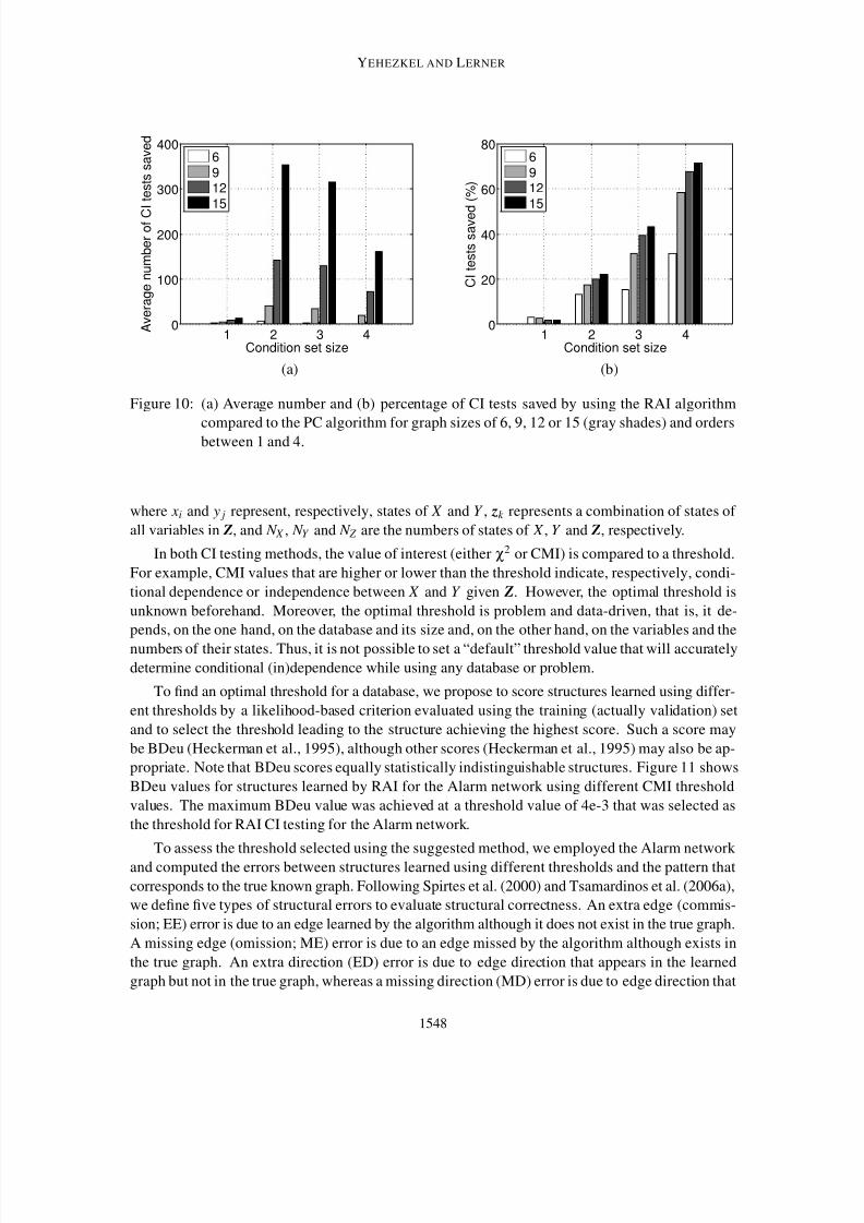
Figure 10: (a) Average number and (b) percentage of CI tests saved by using the RAI algorithm
compared to the PC algorithm for graph sizes of 6, 9, 12 or 15 (gray shades) and ordersbetween 1 and 4.
where xi and y j represent, respectively, states of X and Y , zk represents a combination of states of
all variables in Z, and N X , N Y and N Z are the numbers of states of X , Y and Z, respectively.
In both CI testing methods, the value of interest (either χ2 or CMI) is compared to a threshold.
For example, CMI values that are higher or lower than the threshold indicate, respectively, condi-
tional dependence or independence between X and Y given Z. However, the optimal threshold is
unknown beforehand. Moreover, the optimal threshold is problem and data-driven, that is, it de-
pends, on the one hand, on the database and its size and, on the other hand, on the variables and the
numbers of their states. Thus, it is not possible to set a “default” threshold value that will accurately
determine conditional (in)dependence while using any database or problem.
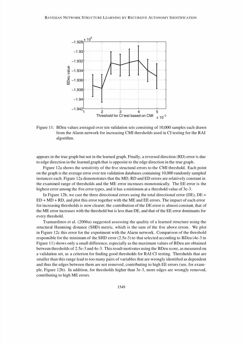
To find an optimal threshold for a database, we propose to score structures learned using differ-
ent thresholds by a likelihood-based criterion evaluated using the training (actually validation) set
and to select the threshold leading to the structure achieving the highest score. Such a score may
be BDeu (Heckerman et al., 1995), although other scores (Heckerman et al., 1995) may also be ap-
propriate. Note that BDeu scores equally statistically indistinguishable structures. Figure 11 shows
BDeu values for structures learned by RAI for the Alarm network using different CMI threshold
values. The maximum BDeu value was achieved at a threshold value of 4e-3 that was selected as
the threshold for RAI CI testing for the Alarm network.
To assess the threshold selected using the suggested method, we employed the Alarm network
and computed the errors between structures learned using different thresholds and the pattern that
corresponds to the true known graph. Following Spirtes et al. (2000) and Tsamardinos et al. (2006a),
we define five types of structural errors to evaluate structural correctness. An extra edge (commis-
sion; EE) error is due to an edge learned by the algorithm although it does not exist in the true graph.
A missing edge (omission; ME) error is due to an edge missed by the algorithm although exists in
the true graph. An extra direction (ED) error is due to edge direction that appears in the learned
graph but not in the true graph, whereas a missing direction (MD) error is due to edge direction that
1548
8/3/2019 01-Bayesian Network Structure Learning by Recursive Autonomy Identification
http://slidepdf.com/reader/full/01-bayesian-network-structure-learning-by-recursive-autonomy-identification 23/44
BAYESIAN NETWORK STRUCTURE LEARNING BY RECURSIVE AUTONOMY IDENTIFICATION
1 2 3 4 5
x 10−3
−1.942
−1.94
−1.938
−1.936
−1.934
−1.932
−1.93
−1.928x 10
5
Threshold for CI test based on CMI
B D e u v a l u e
Figure 11: BDeu values averaged over ten validation sets consisting of 10,000 samples each drawn
from the Alarm network for increasing CMI thresholds used in CI testing for the RAI
algorithm.
appears in the true graph but not in the learned graph. Finally, a reversed direction (RD) error is due
to edge direction in the learned graph that is opposite to the edge direction in the true graph.
Figure 12a shows the sensitivity of the five structural errors to the CMI threshold. Each point
on the graph is the average error over ten validation databases containing 10,000 randomly sampled
instances each. Figure 12a demonstrates that the MD, RD and ED errors are relatively constant inthe examined range of thresholds and the ME error increases monotonically. The EE error is the
highest error among the five error types, and it has a minimum at a threshold value of 3e-3.
In Figure 12b, we cast the three directional errors using the total directional error (DE), DE =
ED + MD + RD, and plot this error together with the ME and EE errors. The impact of each error
for increasing thresholds is now clearer; the contribution of the DE error is almost constant, that of
the ME error increases with the threshold but is less than DE, and that of the EE error dominants for
every threshold.
Tsamardinos et al. (2006a) suggested assessing the quality of a learned structure using the
structural Hamming distance (SHD) metric, which is the sum of the five above errors. We plot
in Figure 12c this error for the experiment with the Alarm network. Comparison of the threshold
responsible for the minimum of the SHD error (2.5e-3) to that selected according to BDeu (4e-3 in
Figure 11) shows only a small difference, especially as the maximum values of BDeu are obtained
between thresholds of 2.5e-3 and 4e-3. This result motivates using the BDeu score, as measured on
a validation set, as a criterion for finding good thresholds for RAI CI testing. Thresholds that are
smaller than this range lead to too many pairs of variables that are wrongly identified as dependent
and thus the edges between them are not removed, contributing to high EE errors (see, for exam-
ple, Figure 12b). In addition, for thresholds higher than 3e-3, more edges are wrongly removed,
contributing to high ME errors.
1549
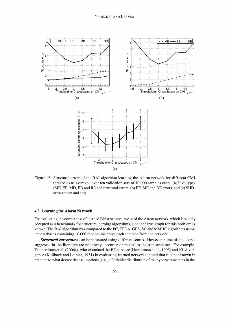
8/3/2019 01-Bayesian Network Structure Learning by Recursive Autonomy Identification
http://slidepdf.com/reader/full/01-bayesian-network-structure-learning-by-recursive-autonomy-identification 24/44
YEHEZKEL AND LERNER
1.5 2 2.5 3 3.5 4 4.5
x 10−3
0
2
4
6
8
Threshold for CI test based on CMI
S t r u c t u r a l e r r o r
ME EE MD ED RD
1.5 2 2.5 3 3.5 4 4.5
x 10−3
1
2
3
4
5
6
7
8
Threshold for CI test based on CMI
S t r u c t u r a l e r r o r
ME EE DE
(a) (b)
1 2 3 4 5
x 10−3
8
10
12
14
16
18
S t r u c t u r a l H a m m i n g d i s t a n c e ( S H D )
Threshold for CI test based on CMI
(c)
Figure 12: Structural errors of the RAI algorithm learning the Alarm network for different CMI
thresholds as averaged over ten validation sets of 10,000 samples each. (a) Five types
(ME, EE, MD, ED and RD) of structural errors, (b) EE, ME and DE errors, and (c) SHD
error (mean and std).
4.3 Learning the Alarm Network
For evaluating the correctness of learned BN structures, we used the Alarm network, which is widely
accepted as a benchmark for structure learning algorithms, since the true graph for this problem is
known. The RAI algorithm was compared to the PC, TPDA, GES, SC and MMHC algorithms using
ten databases containing 10,000 random instances each sampled from the network.
Structural correctness can be measured using different scores. However, some of the scores
suggested in the literature are not always accurate or related to the true structure. For example,
Tsamardinos et al. (2006a), who examined the BDeu score (Heckerman et al., 1995) and KL diver-
gence (Kullback and Leibler, 1951) in evaluating learned networks, noted that it is not known in
practice to what degree the assumptions (e.g., a Dirichlet distribution of the hyperparameters) in the
1550

8/3/2019 01-Bayesian Network Structure Learning by Recursive Autonomy Identification
http://slidepdf.com/reader/full/01-bayesian-network-structure-learning-by-recursive-autonomy-identification 25/44
BAYESIAN NETWORK STRUCTURE LEARNING BY RECURSIVE AUTONOMY IDENTIFICATION
Extra Missing Reversed Directional Extra Missing
Direction Direction Direction Error Edge Edge SHD
(ED) (MD) (RD) (DE) (EE) (ME)
SC 1 9.5 4.6 15.1 4.7 4.5 24.3
MMHC 0.8 3.3 5.7 9.8 2.6 0.7 13.1GES 0.1 0.6 1.2 1.9 2.7 0.8 5.4
TPDA 0 4.2 0 4.2 2.4 2.9 9.5
PC 0 0 0.8 0.8 2.5 1.0 4.3
RAI 0 0 0.3 0.3 1.8 1.4 3.5
Table 1: Structural errors of several algorithms as averaged over 10 databases each containing
10,000 randomly generated instances of the Alarm network. The total directional error
is the sum of three different directional errors, DE=ED+MD+RD, and the SHD error is
DE+EE+ME. Bold font emphasizes the smallest error over all algorithms for each type of
structural error.
basis of the BDeu score hold. Moreover, usually such a score is used in both learning and evaluation
of a structure; hence the score favors algorithms that use it in learning. Tsamardinos et al. (2006a)
also mentioned that both scores do not rely on the true structure. Thus, they suggested the SHD
metric, which is directly related to structural correctness, since it is the sum of the five errors of
Section 4.2. Nevertheless, since SHD can be measured only when the true graph is known, scores
such as BDeu and KL divergence are of great value in practical situations, for example, in classi-
fication problems like those examined in Section 4.5 in which the true graph is not known. These
scores are also beneficial in the determination of algorithm parameters. For example, in Section 4.2
we measured BDeu scores of structures learned using different thresholds in order to select a good
threshold for RAI CI testing.Although SHD sums all five structural errors, we were first interested in examining the contri-
bution of each individual error to the total error. Table 1 summarizes the five structural errors for
each algorithm as averaged over 10 databases of 10,000 instances each sampled from the Alarm
network. These databases are different from those validation databases used for threshold setting.
The table also shows the total directional error, DE, which is the sum of the three directional errors.
Table 1 demonstrates that the lowest EE and DE errors are achieved by the RAI algorithm and the
lowest ME error is accomplished by the MMHC algorithm. Computing SHD shows the advantage
of the RAI (3.5) algorithm over the PC (4.3), TPDA (9.5), GES (5.4), MMHC (13.1) and the SC
(24.3) algorithms. Further, we propose such a table as Table 1 as a useful tool for the identification
of the sources of structural errors of a given structure learning algorithm.
Note that the SHD error weighs each of the five error types equally. We believe that a score
that weighs the five types based on their relative significance to structure learning will be a more
accurate method to evaluate structural correctness; however, deriving such a score is a topic for
future research.
Complexity was evaluated for each of the CB algorithms by measuring the number of CI tests
employed for each order (condition set size) and the total number of log operations. The latter
criterion is proportional to the total number of multiplications, divisions and logarithm evaluations
that is required for calculating the CMI (Equation 2) during CI testing. Figure 13 depicts the average
1551

8/3/2019 01-Bayesian Network Structure Learning by Recursive Autonomy Identification
http://slidepdf.com/reader/full/01-bayesian-network-structure-learning-by-recursive-autonomy-identification 26/44
YEHEZKEL AND LERNER
0 1 2 3 4 50
20
40
60
80
100
Condition set size
C I t e s t r e d u c t i o n ( % )
0%(0)
12%(160)
74%
(422)
97%(243)
100%(64)
100%(4)
0 1 2 3 4 5 6
−100
−50
0
50
100
Condition set size
C I t e s t r e d u c t i o n ( % )
−112%(−587)
54%(170)
94%(112)
100%(28)
100%(1)
100%(6)
0%(0)
(a) (b)
Figure 13: Average percentage (number) of CI tests reduced by using RAI compared to using (a) PC
and (b) TPDA, as a function of the condition set size when learning the Alarm network.
percentage (and number) of CI tests reduced by using the RAI algorithm compared to using the PC
or TPDA algorithms for increasing sizes of the condition sets. The RAI algorithm reduces the
number of CI tests of orders 1 and above required by the PC algorithm and those of orders 2 and
above required by the TPDA algorithm. Moreover, the RAI algorithm completely avoids the use of
CI tests of orders 4 and above and almost completely avoids CI tests of order 3 compared to both
the PC and TPDA algorithms. However, the RAI algorithm performs more CI tests of order 1 than
the TPDA algorithm.
Figure 14 summarizes the total numbers of CI tests and log operations over different condition
set sizes required by each algorithm. The RAI algorithm requires 46% less CI tests than the PCalgorithm and 14% more CI tests (of order 1) than the TPDA algorithm. However, the RAI algorithm
significantly reduces the number of log operations required by the other two algorithms. The PC or
TPDA algorithms require, respectively, an additional 612% or 367% of the number of log operations
required by the RAI algorithm. The reason for this substantial advantage of the RAI algorithm over
both the PC and TPDA algorithms is the saving in CI tests of high orders (see Figure 13). These
tests make use of large condition sets and thus are very expensive computationally.
4.4 Learning Known Networks
In addition to the state-of-art algorithms that were compared in Section 4.3, we include in this
section the OR and GS algorithms. We compare the performance of the RAI algorithm to these
algorithms by learning the structures of known networks employed in real decision support systems
from a wide range of applications. We use known networks described in Tsamardinos et al. (2006a),
which include the Alarm (Beinlich et al., 1989), Barley (Kristensen and Rasmussen, 2002), Child
(Cowell et al., 1999), Hailfinder (Jensen and Jensen, 1996), Insurance (Binder et al., 1997), Mildew
(Jensen and Jensen, 1996) and Munin (Andreassen et al., 1989) networks. All these networks may
be downloaded from the Causal Explorer webpage. The Pigs, Link and Gene networks, which were
also evaluated in Tsamardinos et al. (2006a), are omitted from our experiment due to memory and
1552

8/3/2019 01-Bayesian Network Structure Learning by Recursive Autonomy Identification
http://slidepdf.com/reader/full/01-bayesian-network-structure-learning-by-recursive-autonomy-identification 27/44
BAYESIAN NETWORK STRUCTURE LEARNING BY RECURSIVE AUTONOMY IDENTIFICATION
PC TPDA RAI0
500
1000
1500
2000
2500
3000
N u m b e r o f C I t e s t s
+46%
−14%
Conditionset size
7
6
5
4
3
2
1
0
PC TPDA RAI0
1
2
3
4
x 105
N u m b e r o f l o g o p e
r a t i o n s
+612%
+367%
Condition
set size7
6
5
4
3
2
1
0
(a) (b)
Figure 14: Cumulative numbers of (a) CI tests and (b) log operations required by PC, TPDA, and
RAI for learning the Alarm network. Different gray shades represent different sizes of condition sets. Percentages on tops of the bars are with reference to the RAI algorithm.
run-time limitations of the platform used in our experiment. These limitations are in the computation
of the BDeu scoring function (part of the BNT toolbox) that is used for selecting a threshold for the
RAI CI tests (Section 4.2).
The Casual Explorer webpage also contains larger networks that were created by tiling net-
works, such as the Alarm, Hailfinder, Child and Insurance, 3, 5 and 10 times. In the tiling method
developed by Tsamardinos et al. (2006b), several copies (here 3, 5 and 10) of the same BN are
tiled until reaching a network having a desired number of variables (e.g., Alarm5 has 5 × 37 = 185
variables). The method maintains the structural and probabilistic properties of the original network
but allows the evaluation of the learning algorithm as the number of variables increases without
increasing the complexity of the network. Overall, we downloaded and used nineteen networks, the
most important details of which are shown in Table 2. Further motivation for using these networks
and tiling is given in Tsamardinos et al. (2006a).
Throughout this experiment, we used for each network the same training and test sets as used in
Tsamardinos et al. (2006a), so we could compare the performance of the RAI to all the algorithms
reported in Tsamardinos et al. (2006a). The data in the Causal Explorer webpage are given for each
network using five training sets and five test sets with 500, 1000 and 5,000 samples each. We picked
and downloaded the data sets with the smallest sample size (500), which we believe challenge the
algorithms the most. All the reported results for a network and a learning algorithm in this sub-
section are averages over five experiments in which a different training set was used for training the
learning algorithm and a different test set was used for testing this algorithm.
The RAI algorithm was run by us. CMI thresholds for CI testing corresponded to the maximum
BDeu values were obtained in five runs using five validation sets independent of the training and
test sets, and performances were averaged over the five validation sets. We note that the thresholds
selected according to the maximum BDeu values (Section 4.2) also led to the lowest SHD errors.
The OR algorithm was examined with a maximum number of parents allowed for a node ( k ) of
1553
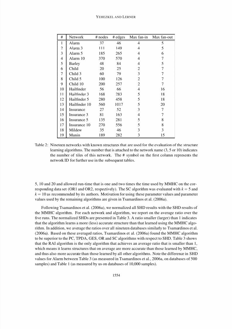
8/3/2019 01-Bayesian Network Structure Learning by Recursive Autonomy Identification
http://slidepdf.com/reader/full/01-bayesian-network-structure-learning-by-recursive-autonomy-identification 28/44
YEHEZKEL AND LERNER
# Network # nodes # edges Max fan-in Max fan-out
1 Alarm 37 46 4 5
2 Alarm 3 111 149 4 5
3 Alarm 5 185 265 4 6
4 Alarm 10 370 570 4 75 Barley 48 84 4 5
6 Child 20 25 2 7
7 Child 3 60 79 3 7
8 Child 5 100 126 2 7
9 Child 10 200 257 2 7
10 Hailfinder 56 66 4 16
11 Hailfinder 3 168 283 5 18
12 Hailfinder 5 280 458 5 18
13 Hailfinder 10 560 1017 5 20
14 Insurance 27 52 3 7
15 Insurance 3 81 163 4 716 Insurance 5 135 281 5 8
17 Insurance 10 270 556 5 8
18 Mildew 35 46 3 3
19 Munin 189 282 3 15
Table 2: Nineteen networks with known structures that are used for the evaluation of the structure
learning algorithms. The number that is attached to the network name (3, 5 or 10) indicates
the number of tiles of this network. The # symbol on the first column represents the
network ID for further use in the subsequent tables.
5, 10 and 20 and allowed run-time that is one and two times the time used by MMHC on the cor-
responding data set (OR1 and OR2, respectively). The SC algorithm was evaluated with k = 5 and
k = 10 as recommended by its authors. Motivation for using these parameter values and parameter
values used by the remaining algorithms are given in Tsamardinos et al. (2006a).
Following Tsamardinos et al. (2006a), we normalized all SHD results with the SHD results of
the MMHC algorithm. For each network and algorithm, we report on the average ratio over the
five runs. The normalized SHDs are presented in Table 3. A ratio smaller (larger) than 1 indicates
that the algorithm learns a more (less) accurate structure than that learned using the MMHC algo-
rithm. In addition, we average the ratios over all nineteen databases similarly to Tsamardinos et al.
(2006a). Based on these averaged ratios, Tsamardinos et al. (2006a) found the MMHC algorithm
to be superior to the PC, TPDA, GES, OR and SC algorithms with respect to SHD. Table 3 shows
that the RAI algorithm is the only algorithm that achieves an average ratio that is smaller than 1,
which means it learns structures that on average are more accurate than those learned by MMHC,
and thus also more accurate than those learned by all other algorithms. Note the difference in SHD
values for Alarm between Table 3 (as measured in Tsamardinos et al., 2006a, on databases of 500
samples) and Table 1 (as measured by us on databases of 10,000 samples).
1554
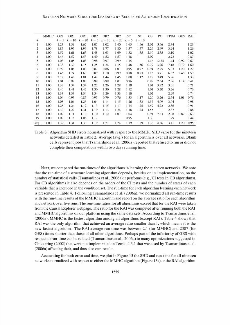
8/3/2019 01-Bayesian Network Structure Learning by Recursive Autonomy Identification
http://slidepdf.com/reader/full/01-bayesian-network-structure-learning-by-recursive-autonomy-identification 29/44
BAYESIAN NETWORK STRUCTURE LEARNING BY RECURSIVE AUTONOMY IDENTIFICATION
MMHC OR1 OR1 OR1 OR2 OR2 OR2 SC SC GS PC TPDA GES RAI
# k = 5 k = 10 k = 20 k = 5 k = 10 k = 20 k = 5 k = 10
1 1.00 1.23 1.39 1.67 1.05 1.02 1.40 1.63 1.66 2.02 3.66 2.34 1.23
2 1.00 1.85 1.95 1.96 1.78 1.77 1.80 1.57 1.57 2.26 2.49 3.94 1.26
3 1.00 1.59 1.61 1.63 1.48 1.63 1.69 1.32 1.35 2.10 2.35 3.10 1.02
4 1.00 1.46 1.52 1.53 1.49 1.52 1.57 1.18 2.09 2.72 0.875 1.00 1.03 1.05 1.08 0.98 0.97 0.99 1.15 1.16 12.34 1.44 0.92 0.67
6 1.00 1.38 1.30 1.15 1.25 1.24 1.15 1.48 1.56 0.79 3.26 7.18 0.79 1.60
7 1.00 0.99 1.06 1.03 0.87 0.86 1.01 0.95 0.97 0.94 2.95 5.03 1.20 1.22
8 1.00 1.45 1.74 1.69 0.89 1.10 0.99 0.88 0.93 1.15 3.71 6.82 2.48 1.59
9 1.00 2.12 1.40 1.81 1.42 1.44 1.45 1.08 1.12 1.19 3.49 5.96 1.33
10 1.00 1.01 0.99 1.03 0.99 0.99 1.01 0.96 0.99 2.64 2.36 1.14 0.41
11 1.00 1.33 1.34 1.34 1.27 1.26 1.28 1.10 1.01 3.92 3.01 0.71
12 1.00 1.40 1.41 1.42 1.30 1.30 1.28 1.12 1.01 5.20 3.26 0.76
13 1.00 1.33 1.33 1.34 1.34 1.29 1.33 1.10 1.02 2.99 0.74
14 1.00 1.04 0.93 0.85 0.95 0.79 0.76 1.33 1.17 1.20 3.26 2.54 1.01 0.76
15 1.00 1.08 1.06 1.25 1.04 1.14 1.15 1.26 1.33 1.57 4.09 3.04 0.98
16 1.00 1.25 1.24 1.12 1.13 1.15 1.17 1.24 1.25 1.59 4.22 2.86 0.91
17 1.00 1.30 1.29 1.31 1.19 1.13 1.24 1.18 1.24 1.55 2.87 0.88
18 1.00 1.09 1.11 1.10 1.10 1.12 1.07 1.04 0.91 7.83 2.08 0.87 0.6319 1.00 1.09 1.16 1.06 1.17 0.95 1.30 1.29 0.44
avg. 1.00 1.32 1.31 1.33 1.19 1.21 1.24 1.19 1.29 1.36 4.36 3.41 1.20 0.95
Table 3: Algorithm SHD errors normalized with respect to the MMHC SHD error for the nineteen
networks detailed in Table 2. Average (avg.) for an algorithm is over all networks. Blank
cells represent jobs that Tsamardinos et al. (2006a) reported that refused to run or did not
complete their computations within two days running time.
Next, we compared the run-times of the algorithms in learning the nineteen networks. We note
that the run-time of a structure learning algorithm depends, besides on its implementation, on the
number of statistical calls (Tsamardinos et al., 2006a) it performs (e.g., CI tests in CB algorithms).
For CB algorithms it also depends on the orders of the CI tests and the number of states of each
variable that is included in the condition set. The run-time for each algorithm learning each network
is presented in Table 4. Following Tsamardinos et al. (2006a), we normalized all run-time results
with the run-time results of the MMHC algorithm and report on the average ratio for each algorithm
and network over five runs. The run-time ratios for all algorithms except that for the RAI were taken
from the Causal Explorer webpage. The ratio for the RAI was computed after running both the RAI
and MMHC algorithms on our platform using the same data sets. According to Tsamardinos et al.
(2006a), MMHC is the fastest algorithm among all algorithms (except RAI). Table 4 shows that
RAI was the only algorithm that achieved an average ratio smaller than 1, which means it is the
new fastest algorithm. The RAI average run-time was between 2.1 (for MMHC) and 2387 (forGES) times shorter than those of all other algorithms. Perhaps part of the inferiority of GES with
respect to run-time can be related (Tsamardinos et al., 2006a) to many optimizations suggested in
Chickering (2002) that were not implemented in Tetrad 4.3.1 that was used by Tsamardinos et al.
(2006a) affecting their, and thus also our, results.
Accounting for both error and time, we plot in Figure 15 the SHD and run-time for all nineteen
networks normalized with respect to either the MMHC algorithm (Figure 15a) or the RAI algorithm
1555

8/3/2019 01-Bayesian Network Structure Learning by Recursive Autonomy Identification
http://slidepdf.com/reader/full/01-bayesian-network-structure-learning-by-recursive-autonomy-identification 30/44
YEHEZKEL AND LERNER
10−2
100
102
10410−1
100
101
102
Runtime divided by the MMHC runtime
S H D d i v i d e d b y t h e M M H C S H D
RAIOther algorithms
(a)
100
102
104
100
101
Runtime divided by the RAI runtime
S H D d i v i d e d b y t h e R A I S H D
(b)
Figure 15: Normalized SHD vs. normalized run-time for all algorithms learning all networks. (a)
Normalization is with respect to the MMHC algorithm (thus MMHC results are at (1,1))and (b) normalization is with respect to the RAI algorithm (thus RAI results are at (1,1)).
The points in the graph correspond to 19 networks (average performance over 5 runs)
and 14 − 1 = 13 algorithms.
1556

8/3/2019 01-Bayesian Network Structure Learning by Recursive Autonomy Identification
http://slidepdf.com/reader/full/01-bayesian-network-structure-learning-by-recursive-autonomy-identification 31/44
BAYESIAN NETWORK STRUCTURE LEARNING BY RECURSIVE AUTONOMY IDENTIFICATION
MMHC OR1 OR1 OR1 OR2 OR2 OR2 SC SC GS PC TPDA GES RAI
# k = 5 k = 10 k = 20 k = 5 k = 10 k = 20 k = 5 k = 10
1 1.00 1.14 1.00 1.07 2.24 2.22 2.33 1.75 16.93 2.17 1.87 3.74 0.69
2 1.00 1.62 1.65 1.64 2.51 2.53 2.63 7.15 9.71 8.16 1.15 12.75 0.52
3 1.00 1.21 1.32 1.33 2.35 2.41 2.48 6.01 6.54 9.80 92.64 9.11 0.59
4 1.00 1.38 1.61 1.43 2.87 2.93 2.77 13.85 71.15 41.81 0.655 1.00 1.26 1.24 1.21 2.29 2.42 2.36 7.36 2.74 89.28 4.10 219.5 0.20
6 1.00 1.61 1.61 1.53 2.39 2.34 3.25 0.64 6.71 1.05 0.82 6.56 31.12 0.25
7 1.00 1.15 1.14 1.06 2.12 2.10 2.18 3.66 8.64 2.44 1.02 10.27 921 0.36
8 1.00 1.12 1.14 1.13 2.10 2.19 2.29 4.16 8.31 5.76 1.05 14.19 3738 0.50
9 1.00 1.34 1.05 1.32 2.20 2.28 2.45 9.97 11.08 12.10 1.36 22.99 0.67
10 1.00 1.20 1.22 1.21 2.31 2.29 2.28 1.58 1.04 1.42 9.31 2690 0.17
11 1.00 1.13 1.15 1.14 2.15 2.21 2.27 4.88 4.96 9.32 32.39 0.65
12 1.00 1.11 1.15 1.17 2.24 2.27 2.19 7.39 10.01 23.14 39.22 0.58
13 1.00 1.18 1.19 1.15 2.94 2.61 2.74 13.77 29.84 99.00 0.85
14 1.00 1.02 1.03 1.03 2.09 2.06 2.05 1.26 15.36 1.02 3.62 10.19 78.06 0.24
15 1.00 1.09 1.13 1.18 2.25 2.38 2.21 2.96 8.50 3.63 59.50 18.87 0.36
16 1.00 1.49 1.48 1.54 2.97 2.95 2.96 5.15 7.88 3.63 173.3 8.67 0.48
17 1.00 1.19 1.12 1.20 2.30 2.35 2.40 10.73 13.95 22.34 32.00 0.64
18 1.00 2.46 2.43 2.55 3.68 3.46 3.68 61.04 5.23 1.76 9.67 343.7 0.7519 1.00 1.05 1.07 1.08 2.09 0.24 0.40 0.27 0.01
avg. 1.00 1.30 1.30 1.31 2.43 2.45 2.53 8.61 10.33 10.39 30.75 20.27 1146 0 .48
Table 4: Algorithm run-times normalized with respect to the MMHC run-time for the nineteen
networks detailed in Table 2. Average (avg.) for an algorithm is over all networks. Blank
cells represent jobs that Tsamardinos et al. (2006a) reported that refused to run or did not
complete their computations within two days running time.
(Figure 15b). Figure 15 demonstrates that the advantage of RAI over all other algorithms is evident
for both the SHD error and the run-time.It is common to consider the statistical calls performed by an algorithm of structure learning as
the major criterion of computational complexity (efficiency) and a major contributor to the algorithm
run-rime. In CB algorithms (e.g., PC, TPDA and RAI), the statistical calls are due to CI tests, and in
S&S algorithms (e.g., GS, GES, SC, OR) the calls are due to the computation of the score. Hybrid
algorithms (e.g., MMHC) have both types of calls. In Table 5, we compare the numbers of calls for
statistical tests performed by the RAI algorithm and computed by us to those of the MMHC, GS, PC
and TPDA, as computed in Tsamardinos et al. (2006a), and downloaded from the Causal Explorer
webpage. We find that for all networks the RAI algorithm performs fewer calls for statistical tests
than all other algorithms. On average over all networks, the RAI algorithm performs only 53% of
the calls for statistical tests performed by the MMHC algorithm, which is the algorithm that required
the fewest calls of all algorithms examined in Tsamardinos et al. (2006a). Figure 16 demonstrates
this advantage of RAI over MMHC graphically using a scatter plot. All points below the x = y line
represent data sets for which the numbers of calls for statistical tests of MMHC are larger than those
of RAI.
Evaluating the statistical significance of the results in Tables 3-5 using Wilcoxon signed-ranks
test (Demsar, 2006) with a confidence level of 0.05, we find the SHD errors of RAI and MMHC to
be not significantly different from each other; however, the RAI run-times and numbers of statistical
calls are significantly shorter than those of the MMHC algorithm.
1557

8/3/2019 01-Bayesian Network Structure Learning by Recursive Autonomy Identification
http://slidepdf.com/reader/full/01-bayesian-network-structure-learning-by-recursive-autonomy-identification 32/44
YEHEZKEL AND LERNER
# MMHC GS PC TPDA RAI
1 1.00 2.42 9.95 1.94 0.81
2 1.00 3.78 2.51 3.34 0.57
3 1.00 4.44 1499.22 3.02 0.67
4 1.00 5.12 2.64 0.755 1.00 1.96 2995.87 1.58 0.34
6 1.00 1.32 3.61 2.92 0.21
7 1.00 2.49 4.61 2.97 0.39
8 1.00 3.25 4.40 3.17 0.51
9 1.00 3.91 5.43 3.13 0.64
10 1.00 1.75 36.54 1.93 0.30
11 1.00 2.57 340.44 1.83 0.72
12 1.00 3.07 1033.86 1.87 0.67
13 1.00 3.40 1.85 0.77
14 1.00 1.32 40.57 2.97 0.27
15 1.00 2.35 1082.45 2.71 0.3916 1.00 3.12 5143.51 2.97 0.49
17 1.00 4.25 3.20 0.63
18 1.00 3.38 10.78 3.49 0.59
19 1.00 1.75 0.91 0.30
avg. 1.00 2.93 814.25 2.55 0.53
Table 5: Number of statistical calls performed by each algorithm normalized by the number of
statistical calls performed by the MMHC algorithm for the nineteen networks detailed
in Table 2. Average (avg.) for an algorithm is over all networks. Blank cells represent
jobs that Tsamardinos et al. (2006a) reported that refused to run or did not complete their
computations within two days running time.
In continuation to Section 4.1, we further analyzed the complexity of RAI (as measured by
the numbers of CI tests performed) according to the CI test orders and the graph size. However,
here we used real rather than synthetic data. We examined the numbers of tests as performed for
different orders for the Child, Insurance, Alarm and Hailfinder networks and their tiled networks.
Using the tiled networks (Tsamardinos et al., 2006b), we could examine the impact of graph size
on the number of tests. Figure 17 shows the cumulative percentage of CI tests for a specific order
out of the total number of CI tests performed for each network. The figure demonstrates that the
percentages of CI tests performed decrease with the CI test order and become small for orders higher
than the max fan-in of the network (see Table 2). These percentages also decrease with the numbers
of nodes in the network (validated on the tiled networks). This is due to a faster increase of the
number of low-order CI tests compared with the number of high-order CI tests as the graph size
increases for all networks except for Hailfinder. For Hailefinder (Figure 17d), the threshold for the
network was different from those of the tiled networks. This led to an increase in the percentage of
high-order CI tests and a decrease in CI tests of order 0 when comparing the Hailfinder network to
its tiled versions. For all the tiled Alarm networks (Figure 17c), CI tests of order 0 nearly sufficed
1558
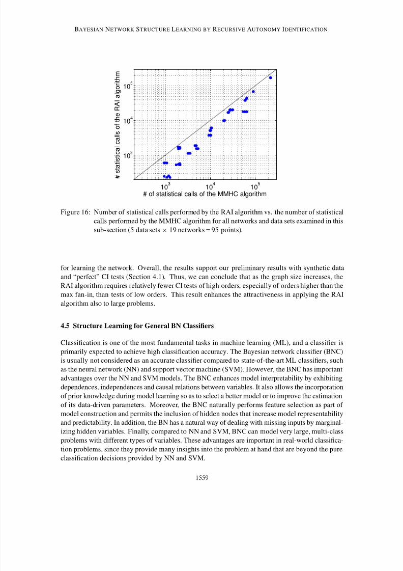
8/3/2019 01-Bayesian Network Structure Learning by Recursive Autonomy Identification
http://slidepdf.com/reader/full/01-bayesian-network-structure-learning-by-recursive-autonomy-identification 33/44
BAYESIAN NETWORK STRUCTURE LEARNING BY RECURSIVE AUTONOMY IDENTIFICATION
103
104
105
103
104
105
# of statistical calls of the MMHC algorithm
# s t a t i s t i c a l c a l l s o f t h e R A I
a l g o r i t h m
Figure 16: Number of statistical calls performed by the RAI algorithm vs. the number of statistical
calls performed by the MMHC algorithm for all networks and data sets examined in this
sub-section (5 data sets × 19 networks = 95 points).
for learning the network. Overall, the results support our preliminary results with synthetic data
and “perfect” CI tests (Section 4.1). Thus, we can conclude that as the graph size increases, the
RAI algorithm requires relatively fewer CI tests of high orders, especially of orders higher than the
max fan-in, than tests of low orders. This result enhances the attractiveness in applying the RAI
algorithm also to large problems.
4.5 Structure Learning for General BN Classifiers
Classification is one of the most fundamental tasks in machine learning (ML), and a classifier is
primarily expected to achieve high classification accuracy. The Bayesian network classifier (BNC)
is usually not considered as an accurate classifier compared to state-of-the-art ML classifiers, such
as the neural network (NN) and support vector machine (SVM). However, the BNC has important
advantages over the NN and SVM models. The BNC enhances model interpretability by exhibiting
dependences, independences and causal relations between variables. It also allows the incorporation
of prior knowledge during model learning so as to select a better model or to improve the estimation
of its data-driven parameters. Moreover, the BNC naturally performs feature selection as part of
model construction and permits the inclusion of hidden nodes that increase model representability
and predictability. In addition, the BN has a natural way of dealing with missing inputs by marginal-
izing hidden variables. Finally, compared to NN and SVM, BNC can model very large, multi-class
problems with different types of variables. These advantages are important in real-world classifica-
tion problems, since they provide many insights into the problem at hand that are beyond the pure
classification decisions provided by NN and SVM.
1559

8/3/2019 01-Bayesian Network Structure Learning by Recursive Autonomy Identification
http://slidepdf.com/reader/full/01-bayesian-network-structure-learning-by-recursive-autonomy-identification 34/44
YEHEZKEL AND LERNER
0 0.5 1 1.5 2 2.5 30.75
0.8
0.85
0.9
0.95
1
CI test order
P e r c e n t a g e f r o m
t h e t o
t a l # C I t e s t s
Child−1Child−3Child−5
Child−10
0 1 2 3
0.65
0.7
0.75
0.8
0.85
0.9
0.95
1
CI test order
P e r c e n t a g e f r o m
t h e t o
t a l # C I t e s t s
Insurance−1Insurance−3Insurance−5
Insurance−10
(a) (b)
0 1 2 3 4 50.4
0.5
0.6
0.7
0.8
0.9
1
CI test order
P e r c e n t a g e f r o m
t h e t o t a l # C I t e s t s
Alarm−1Alarm−3Alarm−5Alarm−10
0 1 2 3 4 5
0.65
0.7
0.75
0.8
0.85
0.9
0.95
1
CI test order
P e r c e n t a g e f r o m
t h e t o t a l # C I t e s t s
Hailfinder−1Hailfinder−3Hailfinder−5
Hailfinder−10
(c) (d)
Figure 17: Cumulative percentages of CI tests out of the total numbers of tests for increasing orders
as performed by the RAI algorithm for the (a) Child, (b) Insurance, (c) Alarm, and (d)
Hailfinder networks including their tiled networks.
We evaluated the RAI complexity, run-time and accuracy when applied to learning a general
BN classifier (Cheng and Greiner, 1999; Friedman et al., 1997) in comparison to other algorithms
of structure learning using nineteen databases of the UCI Repository (Newman et al., 1998) and
Kohavi and John (1997). These databases are detailed in Table 6 with respect to the numbers
of variables, classes and instances in each database. All databases were analyzed using a CV5
experiment, except large databases (e.g., “chess”, “nursery” and “shuttle”), which were analyzed
using the holdout methodology and the common division to training and test sets (Newman et al.,
1998; Friedman et al., 1997; Cheng et al., 1997) as detailed in Table 6. Continuous variables were
discretized using the MLC++ library (Kohavi et al., 1994) and instances with missing values were
removed, as is commonly done.
1560

8/3/2019 01-Bayesian Network Structure Learning by Recursive Autonomy Identification
http://slidepdf.com/reader/full/01-bayesian-network-structure-learning-by-recursive-autonomy-identification 35/44
BAYESIAN NETWORK STRUCTURE LEARNING BY RECURSIVE AUTONOMY IDENTIFICATION
# # # Test # training # testDatabase
variables classes instances methodology instances instances
australian 14 2 690 CV5 552 138
breast 9 2 683 CV5 544 136
car 6 4 1728 CV5 1380 345chess 36 2 3196 holdout 2130 1066
cleve 11 2 296 CV5 236 59
cmc 9 3 1473 CV5 1176 294
corral 6 2 128 CV5 100 25
crx 15 2 653 CV5 520 130
flare C 10 9 1389 CV5 1108 277
iris 4 3 150 CV5 120 30
led7 7 10 3200 CV5 2560 640
mofn 3-7-10 10 2 1324 holdout 300 1024
nursery 8 5 12960 holdout 8640 4320
shuttle (s) 8 7 5800 holdout 3866 1934tic-tac-toe 9 2 958 CV5 764 191
vehicle 18 4 846 CV5 676 169
vote 16 3 435 CV5 348 87
wine 13 3 178 CV5 140 35
zoo 16 7 101 CV5 80 20
Table 6: Databases of the UCI repository (Newman et al., 1998) and of Kohavi and John (1997)
used for evaluating the accuracy of a classifier learned using the RAI algorithm.
Generally for this sub-section, CI tests for RAI and PC were carried out using the χ2 test (Spirtes
et al., 2000) and those for TPDA using the CMI independence test (Equation 2). However, CI tests
for RAI and PC for the “corral”, “nursery” and “vehicle” databases were carried out using the
CMI independence test. In the case of the large “nursery” database, the need to use the CMI test
was due to a Matlab memory limitation in the completion of the χ2 test using the BNT structure
learning package (Leray and Francois, 2004). In the case of the “corral” and “vehicle” databases,
the smallness of the database, together with either the large numbers of classes, variables or states
for each variable, led to low frequencies of instances for many combinations of variable states. In
this case, the implementation of the χ2 test assumes variable dependence (Spirtes et al., 2000) that
prevents the CB (PC, TPDA and RAI) algorithms from removing edges regardless of the order of
the CI test, leading to erroneous decisions. Another test of independence, which is reported to be
more reliable and robust, especially for small databases or large numbers of variables (Dash andDruzdzel, 2003), may constitute another solution in these cases.
Thresholds for the CI tests of the CB algorithms and parameter values for all other algorithms
were chosen for each algorithm and database so as to maximize the classification accuracy on a
validation set selected from the training set or based on the recommendation of the algorithm authors
or of Tsamardinos et al. (2006a). Although using a validation set decreases the size of the training
set, it also eliminates the chance of selecting a threshold or a parameter that causes the model to
1561

8/3/2019 01-Bayesian Network Structure Learning by Recursive Autonomy Identification
http://slidepdf.com/reader/full/01-bayesian-network-structure-learning-by-recursive-autonomy-identification 36/44
YEHEZKEL AND LERNER
overfit the training set at the expense of the test set. If several thresholds/parameters were found
suitable for an algorithm, the threshold/parameter chosen was that leading to the fewest CI tests (in
the case of CB algorithms). For GES and GS there are no parameters to set (except the equivalent
sample size for the BDeu), and for MMHC we used the selections used by the authors in all their
experiments.
Finally, parameter learning was performed by maximum likelihood estimation. Since we were
interested in structure learning, no attempt was made to study estimation methods other than this
simple and most popular generative method (Cooper and Herskovits, 1992; Heckerman, 1995; Yang
and Chang, 2002). Nevertheless, we note that discriminative models for parameter learning have
recently been suggested (Pernkopf and Bilmes, 2005; Roos et al., 2005). These models show an
improvement over generative models when estimating the classification accuracy (Pernkopf and
Bilmes, 2005). We expect that any improvement in classification accuracy gained by using param-
eter learning other than maximum likelihood estimation will be shared by classifiers induced using
any algorithm of structure learning; however, the exact degree of improvement in each case should
be further evaluated.
Complexity of the RAI algorithm was measured by the number of CI tests employed for each
size of the condition set and the cumulative run-time of the CI tests. These two criteria of complexity
were also measured for the PC algorithm, since both the RAI and PC algorithms use the same
implementation of CI testing. Table 7 shows the average number and percentage of CI tests reduced
by the RAI algorithm compared to the PC algorithm for different CI test orders and each database.
An empty entry in the table means that no CI tests of this order are required. A 100% cut in CI tests
for a specific order means that RAI does not need any of the CI tests employed by the PC algorithm
for this order (e.g., orders 2 and above for the “led7” database). It can be seen that for almost all
databases examined, the RAI algorithm avoids most of the CI tests of orders two and above that
are required by the PC algorithm (e.g., the “chess” database). Table 7 also shows the reduction in
the CI test run-time due to the RAI algorithm in comparison to the PC algorithm for all nineteen
databases examined; except for the “australian” database, the cut is measured in tens of percentages
for all databases and for six databases this cut is higher than 70%. Run-time differences between
algorithms may be the result of different implementations. However, since in our case the run-time
is almost entirely based on the number and order of CI tests and RAI has reduced most of the PC CI
tests, especially those of high orders that are expensive in run-time, we consider the above run-time
reduction results to be significant.
Classification accuracy using a BNC has recently been explored extensively in the literature
(Friedman et al., 1997; Grossman and Domingos, 2004; Kontkanen et al., 1999; Pernkopf and
Bilmes, 2005; Roos et al., 2005). By restricting the general inference task of BN to inference
performed on the class variable, we turn a BN into a BNC. First, we use the training data to learn
the structure and then transform the pattern outputted by the algorithm into a DAG (Dor and Tarsi,
1992). Thereafter, we identify the class node Markov blanket and remove from the graph all the
nodes that are not part of this blanket. Now, we could estimate the probabilities comprising the
class node posterior probability, P(C | X ), where X is the set of the Markov blanket variables. Dur-
ing the test, we inferred the state c of the class node C for each test instantiation, X = x, using
the estimated posterior probability. The class c selected was the one that maximized the posterior
probability, meaning that c = argmaxc P(C = c| X = x). By comparing the class maximizing the
posterior probability and the true class, we could compute the classification accuracy.
1562
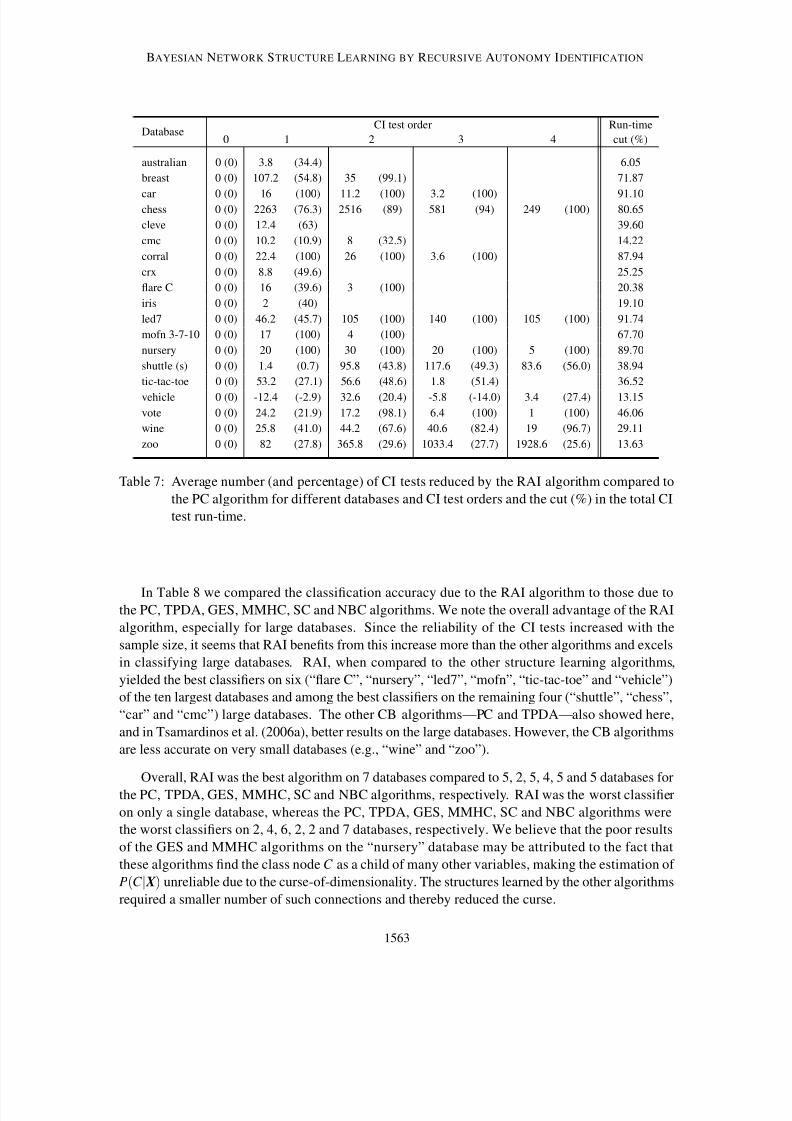
8/3/2019 01-Bayesian Network Structure Learning by Recursive Autonomy Identification
http://slidepdf.com/reader/full/01-bayesian-network-structure-learning-by-recursive-autonomy-identification 37/44
BAYESIAN NETWORK STRUCTURE LEARNING BY RECURSIVE AUTONOMY IDENTIFICATION
CI test order Run-timeDatabase
0 1 2 3 4 cut (%)
australian 0 (0) 3.8 (34.4) 6.05
breast 0 (0) 107.2 (54.8) 35 (99.1) 71.87
car 0 (0) 16 (100) 11.2 (100) 3.2 (100) 91.10chess 0 (0) 2263 (76.3) 2516 (89) 581 (94) 249 (100) 80.65
cleve 0 (0) 12.4 (63) 39.60
cmc 0 (0) 10.2 (10.9) 8 (32.5) 14.22
corral 0 (0) 22.4 (100) 26 (100) 3.6 (100) 87.94
crx 0 (0) 8.8 (49.6) 25.25
flare C 0 (0) 16 (39.6) 3 (100) 20.38
iris 0 (0) 2 (40) 19.10
led7 0 (0) 46.2 (45.7) 105 (100) 140 (100) 105 (100) 91.74
mofn 3-7-10 0 (0) 17 (100) 4 (100) 67.70
nursery 0 (0) 20 (100) 30 (100) 20 (100) 5 (100) 89.70
shuttle (s) 0 (0) 1.4 (0.7) 95.8 (43.8) 117.6 (49.3) 83.6 (56.0) 38.94
tic-tac-toe 0 (0) 53.2 (27.1) 56.6 (48.6) 1.8 (51.4) 36.52
vehicle 0 (0) -12.4 (-2.9) 32.6 (20.4) -5.8 (-14.0) 3.4 (27.4) 13.15
vote 0 (0) 24.2 (21.9) 17.2 (98.1) 6.4 (100) 1 (100) 46.06
wine 0 (0) 25.8 (41.0) 44.2 (67.6) 40.6 (82.4) 19 (96.7) 29.11
zoo 0 (0) 82 (27.8) 365.8 (29.6) 1033.4 (27.7) 1928.6 (25.6) 13.63
Table 7: Average number (and percentage) of CI tests reduced by the RAI algorithm compared to
the PC algorithm for different databases and CI test orders and the cut (%) in the total CI
test run-time.
In Table 8 we compared the classification accuracy due to the RAI algorithm to those due tothe PC, TPDA, GES, MMHC, SC and NBC algorithms. We note the overall advantage of the RAI
algorithm, especially for large databases. Since the reliability of the CI tests increased with the
sample size, it seems that RAI benefits from this increase more than the other algorithms and excels
in classifying large databases. RAI, when compared to the other structure learning algorithms,
yielded the best classifiers on six (“flare C”, “nursery”, “led7”, “mofn”, “tic-tac-toe” and “vehicle”)
of the ten largest databases and among the best classifiers on the remaining four (“shuttle”, “chess”,
“car” and “cmc”) large databases. The other CB algorithms—PC and TPDA—also showed here,
and in Tsamardinos et al. (2006a), better results on the large databases. However, the CB algorithms
are less accurate on very small databases (e.g., “wine” and “zoo”).
Overall, RAI was the best algorithm on 7 databases compared to 5, 2, 5, 4, 5 and 5 databases for
the PC, TPDA, GES, MMHC, SC and NBC algorithms, respectively. RAI was the worst classifier
on only a single database, whereas the PC, TPDA, GES, MMHC, SC and NBC algorithms were
the worst classifiers on 2, 4, 6, 2, 2 and 7 databases, respectively. We believe that the poor results
of the GES and MMHC algorithms on the “nursery” database may be attributed to the fact that
these algorithms find the class node C as a child of many other variables, making the estimation of
P(C | X ) unreliable due to the curse-of-dimensionality. The structures learned by the other algorithms
required a smaller number of such connections and thereby reduced the curse.
1563
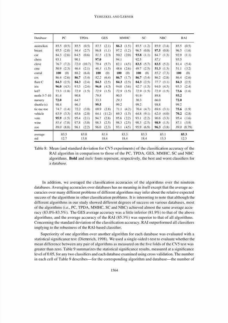
8/3/2019 01-Bayesian Network Structure Learning by Recursive Autonomy Identification
http://slidepdf.com/reader/full/01-bayesian-network-structure-learning-by-recursive-autonomy-identification 38/44
YEHEZKEL AND LERNER
Database PC TPDA GES MMHC SC NBC RAI
australian 85.5 (0.5) 85.5 (0.5) 83.5 (2.1) 86.2 (1.5) 85.5 (1.2) 85.9 (3.4) 85.5 (0.5)
breast 95.5 (2.0) 94.4 (2.7) 96.8 (1.1) 97.2 (1.2) 96.5 (0.8) 97.5 (0.8) 96.5 ( 1.6)
car 84.3 (2.6) 84.5 (0.6) 81.5 (2.3) 90.2 (2.0) 93.8 (1.1) 84.7 (1.3) 92.9 (1.1)chess 93.1 90.1 97.0 94.1 92.5 87.1 93.5
cleve 76.7 (7.2) 72.0 (10.7) 79.4 (5.7) 82.1 (4.5) 83.5 (5.7) 83.5 (5.2) 81.4 ( 5.4)
cmc 50.9 (2.3) 46.4 (2.1) 46.3 (1.5) 48.6 (2.6) 49.7 (2.5) 51.3 (1.3) 51.1 ( 3.2)
corral 100 (0) 88.2 (6.4) 100 (0) 100 (0) 100 (0) 85.2 (7.3) 100 (0)
crx 86.4 (2.6) 86.7 (3.4) 82.2 (6.4) 86.7 (1.7) 86.7 (3.4) 86.2 (2.8) 86.4 (2.6)
flare C 84.3 (2.5) 84.3 (2.4) 84.3 (2.5) 84.3 (2.5) 84.3 (2.5) 77.7 (3.1) 84.3 (2.5)
iris 96.0 (4.3) 93.3 (2.4) 96.0 (4.3) 94.0 (3.6) 92.7 (1.5) 94.0 (4.3) 93.3 (2.4)
led7 73.3 (1.8) 72.9 (1.5) 72.9 (1.5) 72.9 (1.5) 72.9 (1.5) 72.9 (1.5) 73.6 (1.6)
mofn 3-7-10 81.4 90.8 79.8 90.5 91.9 89.8 93.2
nursery 72.0 64.7 33.3 29.3 30.3 66.0 72.0
shuttle (s) 98.4 96.3 99.5 99.2 99.2 98.8 99.2
tic-tac-toe 74.7 (1.4) 72.2 (3.8) 69.9 (2.8) 71.1 (4.2) 70.4 (4.7) 69.6 (3.1) 75.6 (1.9)
vehicle 63.9 (3.3) 65.6 (2.8) 64.1 (11.2) 69.3 (1.5) 64.8 (9.1) 62.0 (4.0) 70.2 (2.8)vote 95.9 (1.5) 95.4 (2.1) 94.7 (2.8) 95.6 ( 2.2) 93.1 (2.2) 90.6 (3.3) 95.4 ( 1.6)
wine 85.4 (7.8) 97.8 (3.0) 98.3 (2.5) 98.3 ( 2.5) 98.3 (2.5) 98.9 (1.5) 87.1 ( 5.9)
zoo 89.0 (8.8) 96.1 (2.2) 96.0 (2.3) 93.1 ( 4.5) 95.9 (6.9) 96.3 (3.8) 89.0 (8.79)
average 83.5 83.0 81.9 83.3 83.3 83.1 85.3
std 12.7 13.8 18.4 18.4 18.4 13.3 12.3
Table 8: Mean (and standard deviation for CV5 experiments) of the classification accuracy of the
RAI algorithm in comparison to those of the PC, TPDA, GES, MMHC, SC and NBC
algorithms. Bold and italic fonts represent, respectively, the best and worst classifiers for
a database.
In addition, we averaged the classification accuracies of the algorithms over the nineteen
databases. Averaging accuracies over databases has no meaning in itself except that the average ac-
curacies over many different problems of different algorithms may infer about the relative expected
success of the algorithms in other classification problems. It is interesting to note that although the
different algorithms in our study showed different degrees of success on various databases, most
of the algorithms (i.e., PC, TPDA, MMHC, SC and NBC) achieved almost the same average accu-
racy (83.0%-83.5%). The GES average accuracy was a little inferior (81.9%) to that of the above
algorithms, and the average accuracy of the RAI (85.3%) was superior to that of all algorithms.
Concerning the standard deviation of the classification accuracy, RAI outperformed all classifiers
implying to the robustness of the RAI-based classifier.
Superiority of one algorithm over another algorithm for each database was evaluated with a
statistical significance test (Dietterich, 1998). We used a single-sided t-test to evaluate whether the
mean difference between any pair of algorithms as measured on the five folds of the CV5 test was
greater than zero. Table 9 summarizes the statistical significance results, measured at a significance
level of 0.05, for any two classifiers and each database examined using cross validation. The number
in each cell of Table 9 describes—for the corresponding algorithm and database—the number of
1564
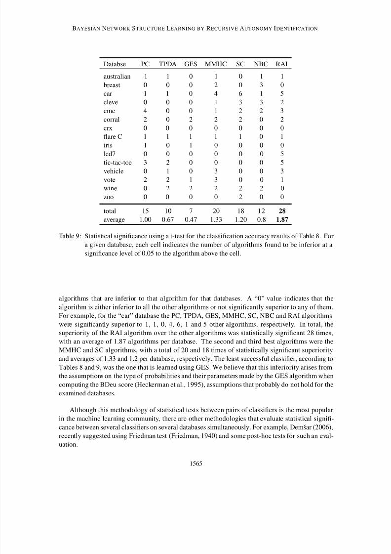
8/3/2019 01-Bayesian Network Structure Learning by Recursive Autonomy Identification
http://slidepdf.com/reader/full/01-bayesian-network-structure-learning-by-recursive-autonomy-identification 39/44
BAYESIAN NETWORK STRUCTURE LEARNING BY RECURSIVE AUTONOMY IDENTIFICATION
Databse PC TPDA GES MMHC SC NBC RAI
australian 1 1 0 1 0 1 1
breast 0 0 0 2 0 3 0
car 1 1 0 4 6 1 5cleve 0 0 0 1 3 3 2
cmc 4 0 0 1 2 2 3
corral 2 0 2 2 2 0 2
crx 0 0 0 0 0 0 0
flare C 1 1 1 1 1 0 1
iris 1 0 1 0 0 0 0
led7 0 0 0 0 0 0 5
tic-tac-toe 3 2 0 0 0 0 5
vehicle 0 1 0 3 0 0 3
vote 2 2 1 3 0 0 1
wine 0 2 2 2 2 2 0
zoo 0 0 0 0 2 0 0
total 15 10 7 20 18 12 28
average 1.00 0.67 0.47 1.33 1.20 0.8 1.87
Table 9: Statistical significance using a t-test for the classification accuracy results of Table 8. For
a given database, each cell indicates the number of algorithms found to be inferior at a
significance level of 0.05 to the algorithm above the cell.
algorithms that are inferior to that algorithm for that databases. A “0” value indicates that the
algorithm is either inferior to all the other algorithms or not significantly superior to any of them.
For example, for the “car” database the PC, TPDA, GES, MMHC, SC, NBC and RAI algorithms
were significantly superior to 1, 1, 0, 4, 6, 1 and 5 other algorithms, respectively. In total, the
superiority of the RAI algorithm over the other algorithms was statistically significant 28 times,
with an average of 1.87 algorithms per database. The second and third best algorithms were the
MMHC and SC algorithms, with a total of 20 and 18 times of statistically significant superiority
and averages of 1.33 and 1.2 per database, respectively. The least successful classifier, according to
Tables 8 and 9, was the one that is learned using GES. We believe that this inferiority arises from
the assumptions on the type of probabilities and their parameters made by the GES algorithm when
computing the BDeu score (Heckerman et al., 1995), assumptions that probably do not hold for the
examined databases.
Although this methodology of statistical tests between pairs of classifiers is the most popular
in the machine learning community, there are other methodologies that evaluate statistical signifi-
cance between several classifiers on several databases simultaneously. For example, Demsar (2006),
recently suggested using Friedman test (Friedman, 1940) and some post-hoc tests for such an eval-
uation.
1565

8/3/2019 01-Bayesian Network Structure Learning by Recursive Autonomy Identification
http://slidepdf.com/reader/full/01-bayesian-network-structure-learning-by-recursive-autonomy-identification 40/44
YEHEZKEL AND LERNER
5. Discussion
The performance of a CB algorithm in BN structure learning depends on the number of conditional
independence tests and the sizes of condition sets involved in these tests. The larger the condition
set, the greater the number of CI tests of high orders that have to be performed and the smaller theiraccuracies.
We propose the CB RAI algorithm that learns a BN structure by performing the following se-
quence of operations: 1) test of CI between nodes and removal of edges related to independences, 2)
edge direction employing orientation rules, and 3) structure decomposition into smaller autonomous
sub-structures. This sequence of operations is performed recursively for each sub-structure, along
with increasing the order of the CI tests. Thereby, the RAI algorithm deals with less potential par-
ents for the nodes on a tested edge and thus uses smaller condition sets that enable the performance
of fewer CI tests of higher orders. This reduces the algorithm run-time and increases its accuracy.
By introducing orientation rules through edge direction in early stages of the algorithm and
following CI tests of lower orders, the graph “backbone” is established using the most reliable
CI tests. Relying on this “backbone” and its directed edges in later stages obviates the need forunnecessary CI tests and enables RAI to be less complex and sensitive to errors.
In this study, we proved the correctness of the RAI algorithm. In addition, we demonstrated
empirically, using synthetically generated networks, samples of nineteen known structures, and
nineteen natural databases used in classification problems, the advantage of the RAI algorithm over
state-of-the-art structure learning algorithms, such as PC, TPDA, GS, GES, OR, SC and MMHC,
with respect to structural correctness, number of statistical calls, run-time and classification accu-
racy. We note that no attempt was made to optimize the parameters of the other algorithms and the
effect of such optimization was not evaluated. This is due to the fact that some of the algorithms
have more than one parameter to optimize and besides, no optimization methods were proposed by
the algorithm inventors. We propose such an optimization method for the RAI algorithm that uses
only the training (validation) data.
We plan to extend our study in several directions. One is the comparison of RAI-based clas-
sifiers to non-BN classifiers, such as the neural network and support vector machine. Second is
the incorporation of different types of prior knowledge (e.g., related to classification) into structure
learning. We also intend to study error correction during learning and to allow the inclusion of
hidden variables to improve representation and facilitate learning with the RAI algorithm.
Acknowledgments
The authors thank the three anonymous reviewers for their thorough reviews and helpful comments
that improved the quality and clarity of the manuscript. The authors also thank the Discovery
Systems Laboratory (DSL) of the Vanderbilt University, TN, for making the Causal Explorer library
of algorithms and the networks tested in Aliferis et al. (2003) freely available. Special thanks due
to Ms. Laura Brown of DSL for the co-operation, helpful discussions and the provision of some
missing results of Aliferis et al. (2003) for comparison. This work was supported, in part, by the
Paul Ivanier Center for Robotics and Production Management, Ben-Gurion University of the Negev,
Beer-Sheva, Israel.
1566
8/3/2019 01-Bayesian Network Structure Learning by Recursive Autonomy Identification
http://slidepdf.com/reader/full/01-bayesian-network-structure-learning-by-recursive-autonomy-identification 41/44
BAYESIAN NETWORK STRUCTURE LEARNING BY RECURSIVE AUTONOMY IDENTIFICATION
References
C. F. Aliferis, I. Tsamardinos, A. Statnikov, and L. E. Brown. Causal Explorer: A causal proba-
bilistic network learning toolkit for biomedical discovery. In Proceedings of the International
Conference on Mathematics and Engineering Techniques in Medicine and Biological Sciences ,
pages 371–376, 2003.
S. Andreassen, F. V. Jensen, S. K. Andersen, B. Falck, U. Kjærulff, M. Woldbye, A. R. Sørensen,
A. Rosenfalck, and F. Jensen. MUNIN—an expert EMG assistant. In John E. Desmedt, editor,
Computer-Aided Electromyography and Expert Systems, chapter 21, pages 255–277. Elsevier
Science Publishers, 1989.
I. A. Beinlich, H. J. Suermondt, R. M. Chavez, and G. F. Cooper. The ALARM monitoring system:
A case study with two probabilistic inference techniques for belief networks. In Proceedings of
the Second European Conference on Artificial Intelligence in Medicine , pages 246–256, 1989.
J. Binder, D. Koller, S. Russell, and K. Kanazawa. Adaptive probabilistic networks with hidden
variables. Machine Learning, 29:213–244, 1997.
J. Cheng. PowerConstructor system. http://www.cs.ualberta.ca/∼jcheng/bnpc.htm, 1998.
J. Cheng and R. Greiner. Comparing Bayesian network classifiers. In Proceedings of the Fifteenth
Conference on Uncertainty in Artificial Intelligence, pages 101–107, 1999.
J. Cheng, D. Bell, and W. Liu. Learning Bayesian networks from data: An efficient approach based
on information theory. In Proceedings of the Sixth ACM International Conference on Information
and Knowledge Management , pages 325–331, 1997.
J. Cheng, C. Hatzis, H. Hayashi, M. Krogel, S. Morishita, D. Page, and J. Sese. KDD cup 2001
report. ACM SIGKDD Explorations Newsletter , 3:47–64, 2002.
D. M. Chickering. Optimal structure identification with greedy search. Journal of Machine Learning
Research, 3:507–554, 2002.
D. M. Chickering, D. Heckerman, and C. Meek. Large-sample learning of Bayesian networks is
NP-hard. Journal of Machine Learning Research, 5:1287–1330, 2004.
G. F. Cooper and E. A. Herskovits. Bayesian method for the induction of probabilistic networks
from data. Machine Learning, 9:309–347, 1992.
R. G. Cowell. Conditions under which conditional independence and scoring methods lead to iden-
tical selection of Bayesian network models. In Proceedings of the Seventeenth Conference on
Uncertainty in Artificial Intelligence, pages 91–97, 2001.
R. G. Cowell, A. P. Dawid, S. L. Lauritzen, and D. J. Spiegelhalter. Probabilistic Networks and
Expert Systems. Springer, 1999.
D. Dash and M. Druzdzel. A hybrid anytime algorithm for the construction of causal models from
sparse sata. In Proceedings of the Fifteenth Conference on Uncertainty in Artificial Intelligence ,
pages 142–149, 1999.
1567

8/3/2019 01-Bayesian Network Structure Learning by Recursive Autonomy Identification
http://slidepdf.com/reader/full/01-bayesian-network-structure-learning-by-recursive-autonomy-identification 42/44
YEHEZKEL AND LERNER
D. Dash and M. Druzdzel. Robust independence testing for constraint-based learning of causal
structure. In Proceedings of the Nineteenth Conference on Uncertainty in Artificial Intelligence,
pages 167–174, 2003.
J. Demsar. Statistical comparisons of classifiers over multiple data sets. Journal of Machine Learn-ing Research, 7:1–30, 2006.
T. G. Dietterich. Approximate statistical tests for comparing supervised classification learning al-
gorithms. Neural Computation, 10:1895–1923, 1998.
D. Dor and M. Tarsi. A simple algorithm to construct a consistent extension of a partially ori-
ented graph. Technical Report R-185, Cognitive Systems Laboratory, UCLA Computer Science
Department, 1992.
M. Friedman. A comparison of alternative tests of significance for the problem of m rankings.
Annals of Mathematical Statistics, 11:86–92, 1940.
N. Friedman, D. Geiger, and M. Goldszmidt. Bayesian network classifiers. Machine Learning, 29:
131–161, 1997.
N. Friedman, I. Nachman, and D. Pe’er. Learning Bayesian network structure from massive datasets:
The “sparse-candidate” algorithm. In Proceedings of the Fifteenth Conference on Uncertainty in
Artificial Intelligence, pages 206–215, 1999.
D. Grossman and P. Domingos. Learning Bayesian network classifiers by maximizing conditional
likelihood. In Proceedings of the Twenty-First International Conference on Machine Learning,
pages 361–368, 2004.
D. Heckerman. A tutorial on learning with Bayesian networks. Technical Report TR-95-06, Mi-crosoft Research, 1995.
D. Heckerman, D. Geiger, and D. M. Chickering. Learning Bayesian networks: The combination
of knowledge and statistical data. Machine Learning, 20:197–243, 1995.
D. Heckerman, C. Meek, and G. F. Cooper. A Bayesian approach to causal discovery. In G. Glymour
and G. Cooper, editors, Computation, Causation and Discovery, pages 141–165. AAAI Press,
1999.
A. Jensen and F. Jensen. MIDAS—an influence diagram for management of mildew in winter
wheat. In Proceedings of the Twelfth Conference on Uncertainty in Artificial Intelligence, pages
349–356, 1996.
R. J. Kennett, K. Korb, and A. E. Nicholson. Seebreeze prediction using Bayesian networks. In
Proceedings of the Fifth Pacific-Asia Conference on Advances in Knowledge Discovery and Data
Mining, pages 148–153, 2001.
R. Kohavi and G. H. John. Wrappers for feature subset selection. Artificial Intelligence, 97:273–
324, 1997.
1568

8/3/2019 01-Bayesian Network Structure Learning by Recursive Autonomy Identification
http://slidepdf.com/reader/full/01-bayesian-network-structure-learning-by-recursive-autonomy-identification 43/44
BAYESIAN NETWORK STRUCTURE LEARNING BY RECURSIVE AUTONOMY IDENTIFICATION
R. Kohavi, G. H. John, R. Long, D. Manley, and K. Pfleger. MLC++: A machine learning library
in C++. In Proceedings of the Sixth International Conference on Tools with AI , pages 740–743,
1994.
P. Kontkanen, P. Myllymaki, T. Sliander, and H. Tirri. On supervised selection of Bayesian net-works. In Proceedings of the Fifteenth Conference on Uncertainty in Artificial Intelligence , pages
334–342, 1999.
K. Kristensen and I. A. Rasmussen. The use of a Bayesian network in the design of a decision
support system for growing malting barley without use of pesticides. Computers and Electronics
in Agriculture, 33:197–217, 2002.
S. Kullback and R. A. Leibler. On information and sufficiency. Annals of Mathematical Statistics,
22:79–86, 1951.
P. Leray and O. Francois. BNT structure learning package: Documentation and experiments. Tech-
nical Report FRE CNRS 2645, Laboratoire PSI, Universite et INSA de Rouen, 2004.
M. Marengoni, C. Jaynes, A. Hanson, and E. Riseman. Ascender II, a visual framework for 3D
reconstruction. In Proceedings of the First International Conference on Computer Vision Systems,
pages 469–488, 1999.
C. Meek. Causal inference and causal explanation with background knowledge. In Proceedings of
the Fifth Conference on Uncertainty in Artificial Intelligence , pages 403–410, 1995.
C. Meek. Graphical Models: Selecting Causal and Statistical Models. PhD thesis, Carnegie Mellon
University, 1997.
A. Moore and W. Wong. Optimal reinsertion: A new search operator for accelerated and more
accurate Bayesian network structure learning. In Twentieth International Conference on Machine
Learning, pages 552–559, 2003.
K. Murphy. The Bayes net toolbox for Matlab. Computing Science and Statistics, 33:331–350,
2001.
D. J. Newman, S. Hettich, C. L. Blake, and C. J. Merz. UCI repository of machine learning
databases, 1998. URL http://www.ics.uci.edu/∼mlearn/MLRepository.html.
J. Pearl. Probabilistic Reasoning in Intelligent Systems: Networks of Plausible Inference. Morgan–
Kaufmann, 1988.
J. Pearl. Causality: Models, Reasoning, and Inference. Cambridge University Press, 2000.
F. Pernkopf and J. Bilmes. Discriminative versus generative parameter and structure learning of
Bayesian network classifiers. In Proceedings of the Twenty-Second International Conference on
Machine Learning, pages 657–664, 2005.
T. Roos, H. Wettig, P. Grunwald, P. Myllymaki, and H. Tirri. On discriminative Bayesian network
classifiers and logistic regression. Machine Learning, 59:267–296, 2005.
1569

8/3/2019 01-Bayesian Network Structure Learning by Recursive Autonomy Identification
http://slidepdf.com/reader/full/01-bayesian-network-structure-learning-by-recursive-autonomy-identification 44/44
YEHEZKEL AND LERNER
M. Singh and M. Valtorta. Construction of Bayesian network structures from data: A brief survey
and an efficient algorithm. International Journal of Approximate Reasoning, 12:111–131, 1995.
P. Spirtes. An anytime algorithm for casual inference. In Proceedings of the Eighth International
Workshop on Artificial Intelligence and Statistics, pages 213–221, 2001.
P. Spirtes and C. Meek. Learning Bayesian networks with discrete variables from data. In Pro-
ceedings of the First International Conference on Knowledge Discovery and Data Mining, pages
294–299, 1995.
P. Spirtes, C. Glymour, and R. Scheines. Causation, Prediction and Search. MIT Press, 2nd edition,
2000.
I. Tsamardinos, L. E. Brown, and C. F. Aliferis. The max-min hill-climbing Bayesian network
structure learning algorithm. Machine Learning, 65:31–78, 2006a.
I. Tsamardinos, A. Statnikov, L. E. Brown, and C. F. Aliferis. Generating realistic large Bayesian
networks by tiling. In Proceedings of the Nineteenth International Florida Artificial Intelligence Research Society Conference, 2006b.
T. Verma and J. Pearl. Equivalence and synthesis of causal models. In Proceedings of the Sixth
Conference on Uncertainty in Artificial Intelligence, pages 220–227, 1990.
S. Yang and K. C. Chang. Comparison of score metrics for Bayesian network learning. IEEE
Transactions on Systems, Man and Cybernetics A, 32:419–428, 2002.
R. Yehezkel and B. Lerner. Recursive autonomy identification for Bayesian network structure learn-
ing. In Proceedings of the Tenth International Workshop on Artificial Intelligence and Statistics ,
pages 429–436, 2005.