001 - international civil aviation organization archive/9689_cons... · 3 no. 1 30/8/02 chapter 1...
TRANSCRIPT


AMENDMENTS
The issue of amendments is announced regularly in the ICAO Journal and in themonthly Supplement to the Catalogue of ICAO Publications and Audio-visualTraining Aids, which holders of this publication should consult. The space belowis provided to keep a record of such amendments.
RECORD OF AMENDMENTS AND CORRIGENDA
AMENDMENTS CORRIGENDA
No. Date Entered by No. Date Entered by
1 30/8/02 ICAO
(ii)
iii
Foreword
Purpose of the manual
In September 1991, the Tenth Air Navigation Conferenceconsidered and endorsed a concept for a future air navi-gation system that would meet the needs of internationalcivil aviation over the next century. The concept, which wasdeveloped by the ICAO Future Air Navigation Systems(FANS) Committee, came to be known as the communica-tions, navigation, and surveillance/air traffic management(CNS/ATM) systems concept and involves a complex andinterrelated set of technologies, dependent, to a largedegree, on satellites.
In follow-up of the work of the FANS Committee andthe Tenth Air Navigation Conference, several activities havetaken or are taking place within and through ICAO asfollows:
— the Council of ICAO has acted on the recom-endations of the Tenth Air Navigation Conferenceto speed up the implementation of CNS/ATM;
— the global coordinated plan for transition to theCNS/ATM systems has been developed;
— the Air Navigation Commission is coordinatingtechnical activities leading to the development ofinternational Standards and RecommendedPractices (SARPs);
— several panels of the Air Navigation Commissionare developing the operational requirements andtechnical specifications necessary for implemen-tation of CNS/ATM systems;
— institutional issues are being addressed by theCouncil of ICAO, the Legal Bureau and con-cerned States; and
— regional planning groups are working on stra-tegies and analyses for their regions.
The CNS/ATM systems concept has reached a highlevel of understanding and acceptance, and efforts are nowbeing directed at the implementation of a seamless, global
air traffic management system. In light of this, the globalplan mentioned above is being revised in a way that willpresent information of a practical nature to guide and assistStates, the ICAO Regional Offices, regional planninggroups, the avionics industry, and operators in planning forthe carriage of airborne equipment required for use withCNS/ATM systems.
The primary objective of this manual is to guideairspace planners, ICAO Regional Offices and the regionalplanning groups and to assist them with implementation ofCNS/ATM systems, particularly in relation to airspaceplanning, implementation of the required navigationperformance (RNP) concept and area navigation techniques.This is in line with the objectives laid out by the Council ofICAO. It is envisioned that the airspace planning method-ology will become a part of a larger document dealing withimplementation issues.
The methodology presented in this document providesa framework by which airspace characteristics, aircraftcapability and traffic demand can be assessed for thepurpose of determining safe separation minima for en-routeoperations. The methodology has been designed to ensurethat the intended safety level for a proposed airspace meetsthe required standard. Airspace planners will be able toassess different scenarios for airspace development.Administrations may use the methodology as a tool to assistthem in determining the sequence and nature of decisionsrequired to establish safe separation minima. However, it isrecognized that, in some cases, application of the method-ology may require risk analysis expertise which may not beavailable in all administrations. In these cases, furthertechnical advice and support should be obtained fromICAO.
Relationship to otherICAO documents
Existing ICAO documents do not indicate methods forquantifying the effect a change of separation minima mayhave on air traffic safety. This document is intended for useby airspace planners as a basis for changing separationminima. It should be read in conjunction with the

iv Manual on Airspace Planning Methodology for the Determination of Separation Minima
No. 130/8/02
International Standards and Recommended Practices, AirTraffic Services (Annex 11 to the Convention on Inter-national Civil Aviation), Attachment A — Material relatingto a method of establishing ATS routes defined by VOR,paragraph 3.1, and Attachment B — Method of establishingATS routes for use by RNAV-equipped aircraft, and the
Procedures for Air Navigation Services — Air TrafficManagement (PANS-ATM, Doc 4444), Chapter 5,Separation Methods and Minima. The Air Traffic ServicesPlanning Manual (Doc 9426) provides guidance on howStates should determine required levels of air trafficservices for their airspace.
v No. 1
30/8/02
TABLE OF CONTENTS
Page
Glossary of Abbreviations . . . . . . . . . . . . . . . . . . . . . 1
Chapter 1. Factors affecting the developmentof an airspace planning methodology . . . . . . . . . . . . 3
Separation considerations . . . . . . . . . . . . . . . . . . . 3Forms of air traffic control service . . . . . . . . . . . . 3Effect of forms of control on separation minima . 4Responsibility for navigation . . . . . . . . . . . . . . . . . 4Determination of separation . . . . . . . . . . . . . . . . . 5Maintenance of separation minima . . . . . . . . . . . . 5Global harmonization of separationminima . . . . . . . . . . . . . . . . . . . . . . . . . . . . . . . . . . 5Required elements of an airspace planningmethodology . . . . . . . . . . . . . . . . . . . . . . . . . . . . . . 5
Chapter 2. Considerations in identifying theneed for change . . . . . . . . . . . . . . . . . . . . . . . . . . . . . 13
Factors affecting the need for change . . . . . . . . . 13Meeting the need for change . . . . . . . . . . . . . . . . 13Cost-benefit analysis . . . . . . . . . . . . . . . . . . . . . . 13
Chapter 3. Description of the current airspaceand the CNS/ATM systems . . . . . . . . . . . . . . . . . . . . 14
Determining separation minima . . . . . . . . . . . . . 14
Chapter 4. Determining the proposed airspaceand CNS/ATM systems . . . . . . . . . . . . . . . . . . . . . . . 16
Factors to be considered in defining theproposed system . . . . . . . . . . . . . . . . . . . . . . . . . . 16Forecasting traffic growth, characteristicsand distribution . . . . . . . . . . . . . . . . . . . . . . . . . . 16
Page
Chapter 5. Identifying the method of safetyassessment for a proposed system . . . . . . . . . . . . . . 17
Safety assessment . . . . . . . . . . . . . . . . . . . . . . . . 17
Chapter 6. Methods of evaluating safety . . . . . . . . 19
Comparison with a reference system . . . . . . . . . . 19Evaluation of system risk against athreshold . . . . . . . . . . . . . . . . . . . . . . . . . . . . . . . . 20
Chapter 7. Modifying the proposed system . . . . . . 27
Risk reduction . . . . . . . . . . . . . . . . . . . . . . . . . . . 27
Chapter 8. Implementation and monitoring . . . . . 29
General . . . . . . . . . . . . . . . . . . . . . . . . . . . . . . . . . 29The need for system performance criteria . . . . . . 29The need for changes in air trafficmanagement procedures . . . . . . . . . . . . . . . . . . . 29The need for approval . . . . . . . . . . . . . . . . . . . . . 29The need for monitoring . . . . . . . . . . . . . . . . . . . 29Air traffic control implementation issues . . . . . . 30Time-scales for implementation . . . . . . . . . . . . . 30The decision to implement . . . . . . . . . . . . . . . . . 31
Appendix 1. A general collision risk model fordistance-based separation on intersecting andcoincident tracks . . . . . . . . . . . . . . . . . . . . . . . . . . . . . 32
Appendix 2. Route structure planning . . . . . . . . . . . 36
Appendix 3. Cost-benefit analysis studies . . . . . . . . 42
Appendix 4. The introduction of a reduced lateralseparation into the NAT Airspace . . . . . . . . . . . . . . . . 46

�� � � � � � �� � � ��� � � � �� �� � � �� � �� � �� � � � � �� ���� � �� � �� �� �� � �� � � ��� � � �� �� � �� �� �� �
No. 130/8/02
Page
Appendix 5. Assessment of longitudinal separationin the Asia/Pacific regions . . . . . . . . . . . . . . . . . . . . . 52
Appendix 6. Example of comparative safetyassessment . . . . . . . . . . . . . . . . . . . . . . . . . . . . . . . . . . 63
Appendix 7. Example of how to trade off variousfactors when comparing a proposed system with areference system . . . . . . . . . . . . . . . . . . . . . . . . . . . . . 66
Appendix 8. A collision risk model fordetermining lateral separation minima forADS-based air traffic control . . . . . . . . . . . . . . . . . . . 69
Appendix 9. The EUROCONTROL hazard/riskanalysis methodology . . . . . . . . . . . . . . . . . . . . . . . . . 85
Appendix 10. Application of risk analysis toairspace planning in Australia . . . . . . . . . . . . . . . . . . . 92
Appendix 11. Air navigation systems analysisand planning methodology . . . . . . . . . . . . . . . . . . . . 104
Page
Appendix 12. Regional airspace planningmethodology . . . . . . . . . . . . . . . . . . . . . . . . . . . . . . . 109
Appendix 13. Analysis to derive lateral navigationperformance requirements for the North Pacific(NOPAC) route system for 50 NM spacingbetween parallel routes . . . . . . . . . . . . . . . . . . . . . . . 113
Appendix 14. Estimating occupancy and therate of accidents due to the loss of plannedlateral separation for the individual componentsof a system of parallel routes . . . . . . . . . . . . . . . . . . 116
Appendix 15. Navigation performancerequirements for the introduction of 30 NMlateral separation in oceanic and remote airspace . . 148
Appendix 16. A method of deriving performancestandards for automatic dependent surveillance(ADS) systems . . . . . . . . . . . . . . . . . . . . . . . . . . . . . . 160
Bibliography . . . . . . . . . . . . . . . . . . . . . . . . . . . . . . . . . .
1 No. 1
30/8/02
Glossary
AACS Australian Airspace Classification SchemeAAIM aircraft autonomous integrity monitoring ACARS ARINC communications addressing and
reporting systemACAS airborne collision avoidance systemADS automatic dependent surveillanceAFTN aeronautical fixed telecommunication
networkAGL above ground levelAIP aeronautical information publication AIRAC aeronautical information regulation and
controlALARP as low as reasonably practicalANT airspace and navigation teamAPANPIRG Asia/Pacific Air Navigation Planning and
Implementation Regional GroupARINC Aeronautical Radio, Inc.ARM airspace risk modelARSR air route surveillance radarATC air traffic controlATCO air traffic controllerATFM air traffic flow managementATM air traffic managementATS air traffic servicesBASI Australian Bureau of Air Safety
InvestigationCAA Civil Aviation AuthorityCAP close approach probabilityCASA Civil Aviation Safety AuthorityCBA cost-benefit analysisCMA Central Monitoring AgencyCMF common mode failuresCNS communications, navigation and
surveillanceCPA circular protected areaCPDLC controller/pilot data link communicationsCTA control areaCTAF common traffic advisory frequencyDDE double double exponentialDME distance measuring equipmentEATCHIP European Air Traffic Control
Harmonization and Integration ProgrammeECAC European Civil Aviation Conference
EURO-CONTROL European Organization for the Safety
of Air NavigationFAA Federal Aviation AdministrationFANS future air navigation systemsFCS flight control systemFDPS flight data processing systemFIR flight information regionFL flight levelFMCS flight management computer systemFMS flight management systemFOM figure of meritGNE gross navigation errorGNSS global navigation satellite system GPS global positioning systemHAZOP formal hazard identification and analysis
sessionsHF high frequencyICAO International Civil Aviation OrganizationIEC International Electrotechnical CommissionIFR instrument flight rulesIMC instrument meteorological conditionsIOACG Indian Ocean Air Traffic Services Co-
ordinating GroupIRR internal rate of returnISPACG Informal South Pacific Air Traffic Services
Co-ordinating GroupLORAN long-range air navigation (system)LSSR long-range secondary surveillance radarMAPT missed approach pointMASPS minimum aircraft system performance
standardsMBZ mandatory broadcast zoneMNPS minimum navigation performance
specificationsMOPS minimum operational performance
specificationMWG Mathematicians Working GroupNAT North AtlanticNAT SPG North Atlantic Systems Planning GroupNM nautical milesNOPAC North PacificNOTAM notice to airmen
2 Manual on Airspace Planning Methodology for the Determination of Separation Minima
No. 130/8/02
NPV net present valueNSW New South WalesNWPIE non-waypoint-insertion gross errorOACC oceanic area control centreOH&S occupational health and safetyOR operational requirementOTS organized track systemPANS-ATM Procedures for Air Navigation Services —
Air Traffic ManagementR&D research and developmentRAIM receiver autonomous integrity monitoringRDPS radar data processing systemRGCSP Review of the General Concept of
Separation PanelRLRS reduced lateral route spacingRNAV area navigationRNDSG route network development sub-groupRNP required navigation performanceRPT regular public transportRTCA Radio Technical Commission for
Aeronautics
RVSM reduced vertical separation minimumSARPs Standards and Recommended PracticesSATCOM satellite communicationSID standard instrument departureSRD standard radar departureSSR secondary surveillance radarSTAR standard instrument arrival routeSUPPS Supplementary ProceduresTCAS traffic alert and collision avoidance systemTLS target level of safetyTMA terminal control areaUTC coordinated universal timeVFR visual flight rulesVHF very high frequencyVMC visual meteorological conditionsVOR VHF omnidirectional radio range WG working groupWP working paperWPIE waypoint-insertion gross error

3 No. 130/8/02
Chapter 1FACTORS AFFECTING THE DEVELOPMENT OF
AN AIRSPACE PLANNING METHODOLOGY
SEPARATION CONSIDERATIONS
1.1 Separation is the generic term used to describeaction on the part of air traffic services (ATS) to keepaircraft operating in the same general area at such distancesfrom each other that the risk of collision is maintainedbelow an acceptable safe level. Such separation can beapplied horizontally and vertically. Separation in thehorizontal plane can be achieved either longitudinally (byspacing aircraft behind each other at a specified distance,which may be expressed in flying time) or laterally (byspacing aircraft side by side at a specified distance fromeach other, or by specifying the width of the protectedairspace on either side of an air route centre line). Verticalseparation is achieved by requiring aircraft using prescribedaltimeter setting procedures to operate at different levelsexpressed in terms of flight levels or altitudes.
Note.— Guidance material on reduced vertical separa-tion minima (RVSM) is available in (Doc 9574) Manual onImplementation of a 300 m (1 000 ft) Vertical SeparationMinimum Between FL 290 and FL 410 Inclusive.
1.2 The required separation between aircraft isgenerally expressed in terms of minimum distances in eachdimension which should not be simultaneously infringed.In the case of horizontal separation, the minimum distancecan be expressed in either nautical miles (NM), degrees ofangular displacement or, in the longitudinal dimension, asvalues of either time-based or distance-based minima, byuse of distance measuring equipment (DME), areanavigation (RNAV), radar or automatic dependent surveil-lance (ADS) respectively (Doc 4444, Procedures for AirNavigation Services — Air Traffic Management, PANS-ATM). Vertically, the minimum is expressed in eithermetres, feet or flight levels.
1.3 Under some circumstances, in specified airspacesand subject to regional agreement, composite separation
consisting of an element of horizontal separation combinedwith an element of vertical separation may be appliedbetween aircraft (Doc 9426, Air Traffic Services PlanningManual, Part II, Section 2, Chapter 3 refers).
1.4 When planning airspace and air routes that are notprovided with an air traffic control (ATC) service (onlyflight information service or air traffic advisory service),safe separation of aircraft can also be assured by the use ofstandard separation minima. In the event that an ATCservice is subsequently introduced, the use of the sameprocess will facilitate implementation and integration withadjacent airspace systems.
FORMS OF AIR TRAFFICCONTROL SERVICE
1.5 To provide separation, ATC uses two forms ofcontrol: procedural and radar. Procedural control isgenerally understood to be the application of separationbased solely on position information received from theaircraft via air-ground communications. It is envisaged thattechnologies utilizing ADS, where airborne navigationaldata are made available to ATC by data link techniques, willprovide enhancements to procedural control. The intro-duction of ADS into the procedural ATC environmentoffers the potential for more frequent position updates aswell as information on the future intent of the aircraft. In anenvironment where position reports are communicateddirectly from the aircraft to ATC, and where ATC isautomatically kept up to date on the intentions of theaircraft, significant reductions in separation minima shouldbe possible.
1.6 Radar control is based on radar-displayed positioninformation. Horizontal separation is achieved by main-taining a specified horizontal distance between radar returnsfrom different aircraft. Vertical separation may also be

4 Manual on Airspace Planning Methodology for the Determination of Separation Minima
No. 130/8/02
applied between radar returns. This may be enhanced inareas where secondary surveillance radar (SSR) is used (itshould be noted that the information on height provided ina radar environment using SSR and Mode C is a form ofdependent surveillance whereby the aircraft’s height isderived from the altimetry systems on individual aircraft).
EFFECT OF FORMSOF CONTROL ON
SEPARATION MINIMA
1.7 There is a significant difference between theseparation minima used when applying strictly proceduralcontrol methods and those used under radar control. Theseparation minima used under procedural control takes intoaccount that ATC decisions are based on a “snap-shot”picture of the situation and the controller ensures that allaircraft under control are suitably separated from eachother. Pilots’ estimates of their flight progress mustindicate that the separation established will continue untilsuch time as ATC is in a position to again review the trafficsituation. The separation minima used in this case musttherefore ensure that, even in the worst case conditions (i.e.between successive snap-shots), the required minima canbe maintained, or re-established should they becomedegraded. It should be understood, however, that the use ofthe procedural control method does not relieve controllersfrom their obligations to monitor the traffic situationcontinuously.
1.8 In the case of radar control, ATC is provided withfrequently updated real-time information on the position ofaircraft, making it possible when required to use signi-ficantly smaller separation minima. However, the minimaused under these conditions must also take into account thefact that little information is provided from radar data aloneon the future intent of aircraft. Further information on thedetermination of appropriate radar separation is providedin Annex 11 and the PANS-ATM.
1.9 Effect of tactical radar control. In a radarenvironment, when appropriate lateral spacing existsbetween adjacent routes, such routes may be operated bythe controller as separate entities. In this case, when anaircraft is cleared and established on an ATS route:
a) the pilot is responsible for adhering to the centreline;
b) aircraft established on adjacent routes are separatedby the appropriate spacing between the routes; and
c) the controller’s role is primarily one of monitoringthe progress of cleared aircraft.
1.10 In a radar environment, when appropriate lateralspacing does not exist between routes, aircraft may beseparated from those on adjacent routes, by the controllerapplying the minimum radar separation, specified by theATS authority. In such cases, the use of automated warningtools, such as deviation alert and short-term conflict alert(STCA), may allow the controller to operate the routes witha degree of independence. Thereby, the controller’s primaryrole may also become that of monitoring the progress ofcleared aircraft on each route, thus allowing for more activecontrol when required, as in the case of climbing anddescending traffic. The time required, therefore, to detectand resolve a deviation and/or potential conflict will dependon a number of factors which include:
a) controller workload;
b) availability of automated warning tools, e.g.deviation alert, STCA;
c) pilot/controller reaction time to initiate and executecorrective action;
d) delays in pilot/controller communications;
e) the resolution and accuracy of the system; and
f) aircraft manoeuvre response time (dependent onaircraft speed and height).
1.11 The introduction of ADS into the proceduralATC environment offers the potential for more frequentposition updates as well as information on the future intentof the aircraft. In an ADS environment where positionreports are communicated directly from the aircraft to ATC,and where ATC is automatically kept up to date on theintentions of the aircraft, significant reductions in separationminima should be possible. The extent of separationreductions need to be determined by either collision riskmodelling or the other techniques detailed in the method-ology in this manual.
RESPONSIBILITY FOR NAVIGATION
1.12 The ATC system is based on the principle thatthe responsibility for navigation is vested with the pilot. The
Chapter 1. Factors affecting the development of an airspace planning methodology 5
No. 130/8/02
ATC system does not normally assume responsibility forthe navigation of aircraft except in certain prescribedinstances (e.g. radar vectoring) when the air trafficcontroller is in a better position to obtain information on anaircraft’s position relative to other aircraft, or when the airtraffic controller determines the need to resolve a potentialhazard.
DETERMINATION OF SEPARATION
1.13 The determination of vertical separation or time-and distance-based longitudinal separation minima shouldbe based on the quality of information available to ATCand the pilot. Decision, coordination and transmissiontimes may have an influence on the application oflongitudinal separation minima, particularly where directpilot-controller communications are not available. Thedetermination of lateral separation in a procedural environ-ment should be based primarily on the accuracy with whichpilots can adhere to an assigned track. When an ATCintervention capability is available, its influence on lateralseparation minima should be assessed.
MAINTENANCE OFSEPARATION MINIMA
1.14 Determination of the appropriate prescribedseparation minima is a complex process and it is necessaryto take into account the factors listed in 1.16, 1.17 and1.18. Once the responsible authority establishes separationminima, it is incumbent upon ATC to ensure that these arenot compromised. In addition, when evaluating airspacesafety and efficiency, it is not only the minima that areimportant, but also how frequently separations close to theminima are applied in practice.
GLOBAL HARMONIZATION OFSEPARATION MINIMA
1.15 From the early days of ICAO, it was agreed thatto facilitate global harmonization, separation minimashould be established internationally and that such minimashould only be changed through international agreement.Annex 11 specifies that the minima established by ICAOare published in the PANS-ATM and minima establishedby Regional Agreement are published in Doc 7030,Regional Supplementary Procedures (SUPPS). This material
forms the initial source of reference material from whichairspace planners may directly derive appropriate minima.
REQUIRED ELEMENTS OF ANAIRSPACE PLANNING METHODOLOGY
1.16 The primary aim of airspace system design is toprovide safe aircraft operations for the intended phases offlight. This includes navigation along the intended flightpath, obstacle avoidance and support of separation stan-dards that accommodate required system capacity andsafety.
1.17 Three of the main interdependent parameters thataffect the achievement of such a predetermined level ofairspace system safety (target level of safety — TLS) for agiven traffic density are:
a) aircraft navigation performance;
b) ground and airborne communications performance;and
c) surveillance performance.
1.18 These performance capabilities are used todetermine airspace design (separation minima/route spacing/sectorization), instrument procedures and air traffic controlintervention capability. An increase or decrease in anysingle parameter may result in a corresponding increase ordecrease in some or all of the other parameters. As aircraftand system capabilities improve, it is expected that corres-ponding improvements in system safety will be realized.The methodology for determination of en-route separationminima allows a trade-off between the system aspects ofseparation, navigation and intervention to ensure that anagreed TLS is satisfied.
1.19 In recent years, most of the work on separationminima between aircraft has been based on mathematical/statistical analyses. Such work has been extremely useful inassessing the probable safety of proposed separationminima and is intended to support informed decisions basedon sound operational judgement. This document includespossible methodologies to assess traffic safety in relation toseparation minima. The methodology for determiningseparation minima is based on special mathematical models,which determine the correlation between elements such ascollision risk, separation minima, airspace design, air routenetwork characteristics, flow parameters, interventioncapability and communication, navigation and surveillance
6 Manual on Airspace Planning Methodology for the Determination of Separation Minima
No. 130/8/02
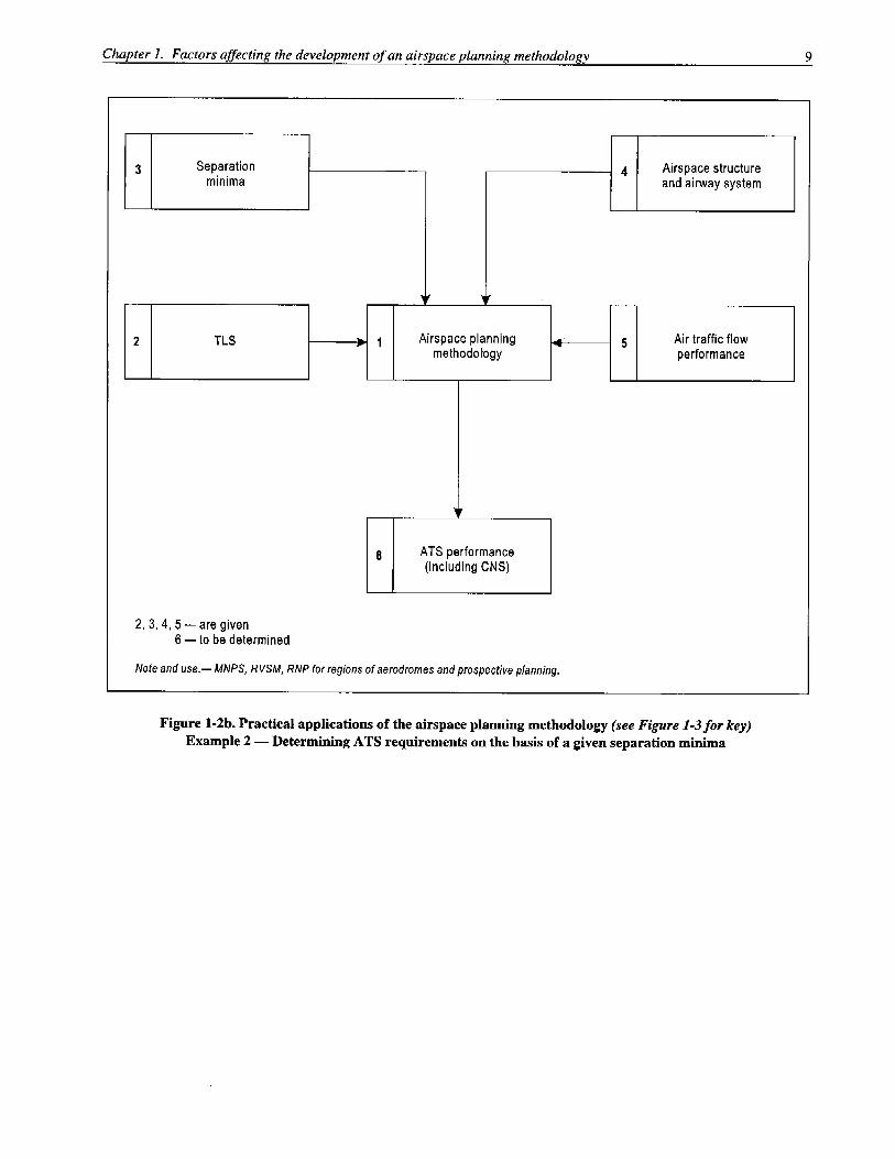
equipment performance. The airspace planning method-ology is sufficiently universal to be used not only fordetermining separation minima, but also for safely imple-menting ATS upgrades in situations where separationminima are intended to remain unchanged, for example:determination of communications, navigation, and surveil-lance (CNS) requirements for a given TLS and separationminimum; estimation of the influence of airspace structurechanges on system safety; and determination of air trafficsystem capacity limits.
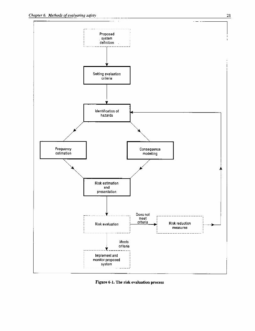
1.20 In this document the methodology described fordetermining safe separation minima is an iterative method.The flow diagram in Figure 1-1 shows the relationshipbetween the following fundamental elements of themethodology:
a) identification of the need for change;
b) determination of the proposed system;
c) identification of the method of safety assessment;
d) evaluation of the risk;
e) satisfaction of safety criteria;
f) modification of the proposed system; and
g) implementation and monitoring of the proposedsystem.
1.21 Airspace planners may use the flow diagram asa tool to assist them in determining the sequence and natureof the decisions required to derive safe separation minimaor for safely implementing ATS upgrades in their airspace,described in 1.19 above. Some practical applications of howthe airspace planning methodology can be used to derive airtraffic system solutions are shown in Figures 1-2a to 1-2d.Detailed guidance on each of the elements of themethodology is given in the remaining chapters.


Chapter 6. Methods of evaluating safety 23
No. 130/8/02
Lateral navigation performance
The lateral navigation performance of the aircraftpopulation determines the lateral overlapprobability. This is a measure of the likelihood thattwo aircraft, which are nominally separated, are infact in lateral overlap. This parameter is a keyelement in determining the lateral collision risk. Thelateral collision risk is directly proportional to thelateral overlap probability for two aircraft nominallyseparated by the lateral separation minimum.
In a procedural airspace with a parallel track systemand dependent surveillance, the lateral overlap prob-ability is affected by both the typical andnon-typical navigation performance. Typicalperformance is used here to describe the usual smallerrors in position which occur when navigationsystems are operating correctly; the non-typicalperformance arises either due to navigation systemfailures or human error and can result in very largedeviations from the correct position. The non-typicalperformance can be measured in terms of theproportion of flight time spent at a distance greaterthan half the lateral separation minimum from thecorrect track and by the proportion of aircraft flighttime spent near to the centre line of another route.
The relative effect of these two sources of error onthe lateral overlap probability may vary from airspaceto airspace. For example, in the North Atlanticminimum navigation performance specifications(NAT MNPS) airspace, the lateral separation mini-mum is so large that the non-typical performancecontributes, by far, the largest part to the lateraloverlap probability and hence to the collision risk.When planning a parallel track system, great careshould be exercised in establishing separations largeenough to eliminate virtually all risk due to typicalerrors, and characterizing and then controlling thelevel of non-typical navigational performance.
Lateral navigation is also important when assessingthe collision risk in the longitudinal dimension,although in this case it is the nominal performancethat is most important. This is because iflongitudinal separation is eroded between twoaircraft nominally flying on the same track, acollision can occur only if the two aircraft are inlateral overlap. The longitudinal collision risk isdirectly proportional to the lateral overlap probabilitybetween two aircraft nominally on the same track.The effect of changing the standard deviation of thepopulation (approximately half of the RNP value if
it is assumed that the core distribution is a Gaussiandistribution) is shown in Table 6-1. It should benoted that improving lateral navigation actuallyincreases the longitudinal collision risk.
Table 6-1. Lateral overlap probabilities RNP value
RNP value Standarddeviation of the
population(NM)
Lateral overlapprobability
1 0.51 0.0301
4 2.04 0.0075
5* 2.55 0.0060
10* 5.10 0l.0030
12.6 6.43 0.0024
20 10.20 0.0015
* Example of a regional application
Longitudinal navigation performance
The longitudinal collision risk is also dependenton the typical along-track navigational performance,which determines the likelihood that longitudinalseparation will be lost. Therefore, it is important toconstrain the along-track performance of the aircraftpopulation. In a typical oceanic airspace, wherepilot reports at waypoints are used, the maintenanceof longitudinal separation is dependent not only onthe ability of the pilots to determine the aircraft’slongitudinal position, but also on the accuracy withwhich all flights in the system measure time. Theaccuracy of position measurement can be controlledby selecting an RNP value. The accuracy of timemeasurement can be controlled by specifying indivi-dual aircraft time-keeping accuracy. When boththese factors are controlled, they combine to limitthe variation in inter-aircraft spacing, thus alsoreducing the risk.
In procedural airspace the minimum longitudinalseparation is often specified in terms of theminimum time between consecutive aircraft on thesame track. The longitudinal separation measured innautical miles then depends upon the speed of theaircraft concerned. Maintaining the correctlongitudinal separation on long en-route tracks canbe simplified by the application of speed controls,
24 Manual on Airspace Planning Methodology for the Determination of Separation Minima
No. 130/8/02
e.g. Mach number technique, which requires allaircraft in the system to maintain constant speeds,(Doc 9426, Part II, Section 2, Chapter 2 refers). Theinitial longitudinal separation on entry to a tracksystem is then based on the relative speed betweeneach consecutive pair of aircraft and is set in orderto ensure that the minimum separation on the trackwill not be infringed throughout the flight. Theapplication of Mach number technique reduces thevariability of spacing between aircraft and reducesthe requirement for ATC intervention to correct thisspacing.
Vertical navigation performance
Vertical navigation performance is determined bythe altitude-maintenance capability of the aircraftpopulation. Vertical navigation performance is notonly important for setting vertical separationrequirements (Doc 9574 refers), but the nominalperformance also affects the risk in the lateral andlongitudinal dimensions. If separation is lost in bothof these dimensions between aircraft nominally atthe same level, a collision will only result if bothaircraft are also in vertical overlap. The collisionrisk in the longitudinal or lateral dimensions istherefore directly proportional to the verticaloverlap probability between two aircraft nominallyat the same altitude.
3) Effects of surveillance and communications
The collision risk in a given airspace is directlyaffected by the capability of ATC to detect aircrafton conflicting tracks and to correct the situationbefore a collision can occur. This interventioncapability is determined by the efficiency of thesurveillance and communication systems availableto the air traffic controller. Safe separation minimain an airspace are closely linked to the means ofsurveillance and communication available to ATC.As airspaces change from strictly proceduralsystems, improvements in surveillance, com-munications and ground-based automation combineto form an enhanced decision-support system for thecontroller and allow progressively smallerseparations to be used safely.
A principal feature of the communication linksbetween pilot and controller, which affects the mini-mum separation that can be safely maintained, is thedelay in transferring the desired information. Thereliability, availability and integrity of the com-munication subsystem must also be assessed to
understand its function in the overall decision-support system. In the case where the communica-tions link carries traffic for dependent surveillanceactivities, the communications performance para-meters are directly related to the surveillance func-tion, e.g. where ADS is used as a primary surveil-lance tool, the performance of the applied data linkhas a direct influence on the surveillance andintervention capability and thus on the achievablesafe separation minima. Appendix 8 summarizes amethod for determining lateral separation minima inan ADS-based ATC system.
Information on the status and position of aircraft isessential for ATC. The provision of this informationcan range from pilot reports at intervals of 30 minutesor more, to radar data updated every 4-6 seconds.Whatever the system being used, its reliability,integrity and availability must be assessed, as wellas the accuracy of the information and any delays inthe presentation of the information to ATC.
The delay in presenting information to the controlleris related to the update rate of the surveillancesystem and in some cases may be produced byautomation (for instance in resolving the non-synchronization of the timing of reports fromdifferent surveillance systems). In addition topresentation to the controller, some systems employconformance checking for individual aircraft orconflict prediction for pairs of aircraft. The selec-tion of the threshold for these decision aids andtheir associated alarm levels will have an effect onthe system safety.
The additional margin of safety provided by con-troller intervention can be assessed in part byestimating the delay from the time that the controllerperceives that a collision hazard exists until instruc-tions are communicated and the aircraft responds.
Setting evaluation criteria
6.13 In order to evaluate the estimate of collision risk,this should be compared to a maximum tolerable collisionrisk for the system. Determining this level of risk is anindependent process involving decision makers whorepresent State authorities, regional authorities or ICAOtechnical panels. The maximum tolerable risk is normallyexpressed in terms of a TLS. In the past, when applied toen-route collision risk, the TLS had been expressed in termsof the number of fatal accidents per flight hour, which couldresult from collisions between aircraft (where a collision


Appendix 1A GENERAL COLLISION RISK MODELFOR DISTANCE-BASED SEPARATION
ON INTERSECTING AND COINCIDENT TRACKS
1. INTRODUCTION
This appendix presents a new model for the analysis of collision risk applicable to distance-based separationof aircraft on both intersecting tracks as well as identical tracks. The model is based on the well-establishedReich Model (see references 19, 20, 21), but the derivation presented here is new and indicates the generalapplicability of the method.
2. METHODOLOGY
2.1 Suppose that a randomly chosen pair of aircraft, not necessarily at the same level, is crossing an oceanon either the same identical track or on tracks that intersect. We denote by TC the average flying time tocomplete the crossing. Let the notation Prob{X} mean the probability of X occurring, and define
Cp = Prob{the pair collides during the oceanic crossing}. (1)
2.2 As in the Reich model, we represent the aircraft by simple geometric shapes. In this appendix we willassume the aircraft are circular cylinders of diameter �xy and height �z. Again, as in the Reich model, we usean equivalent geometry where one aircraft, aircraft 1 in this explanation, is a cylinder of �xy radius and height2�z, which we denote C, and the other aircraft, aircraft 2, is a point particle, which we denote P. It is clear thatfor a collision to occur P must enter C through its vertical side or through the top or bottom. It is also clear thata horizontal overlap of the two aircraft occurs when P enters the infinite cylinder of radius �xy obtained byextending upwards and downwards the cylinder representing aircraft 1. Thus,
Cp = Prob{P enters C | P enters infinite cylinder} × HOP(TC) (2)
where HOP(TC) denotes the probability the pair of aircraft will have a horizontal overlap during the oceaniccrossing.
2.3 Now to calculate Prob{P enters C | P enters infinite cylinder}, note that xy, the average horizontal path�
length through a cylinder of radius �xy, is given by
(3).2xyxy λπ=�
No. 1 3230/8/02
Appendix 1. A general collision risk model for distance-based separationon intersecting and coincident tracks 33
No. 1
30/8/02
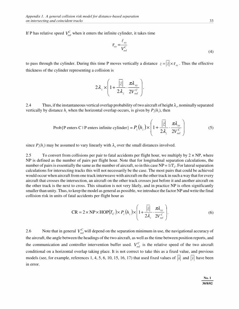
If P has relative speed when it enters the infinite cylinder, it takes timeCrelV
(4)Crel
xyxy V
�=τ
to pass through the cylinder. During this time P moves vertically a distance . Thus the effectivexyzz τ×= �thickness of the cylinder representing a collision is
.22
12 ��
�
�
��
�
�⋅+×
Crel
xy
zz
V
z πλλ
λ�
2.4 Thus, if the instantaneous vertical overlap probability of two aircraft of height �z, nominally separatedvertically by distance hz when the horizontal overlap occurs, is given by Pz(hz), then
Prob{P enters C | P enters infinite cylinder} = (5)( )��
�
�
��
�
�⋅+× C
rel
xy
zzz V
zhP
221
πλλ�
since Pz(hz) may be assumed to vary linearly with �z over the small distances involved.
2.5 To convert from collisions per pair to fatal accidents per flight hour, we multiply by 2 × NP, whereNP is defined as the number of pairs per flight hour. Note that for longitudinal separation calculations, thenumber of pairs is essentially the same as the number of aircraft, so in this case NP = 1/TC. For lateral separationcalculations for intersecting tracks this will not necessarily be the case. The most pairs that could be achievedwould occur when aircraft from one track interweave with aircraft on the other track in such a way that for everyaircraft that crosses the intersection, an aircraft on the other track crosses just before it and another aircraft onthe other track is the next to cross. This situation is not very likely, and in practice NP is often significantlysmaller than unity. Thus, to keep the model as general as possible, we introduce the factor NP and write the finalcollision risk in units of fatal accidents per flight hour as
. (6)( ) ( )��
�
�
��
�
�⋅+××××=
Crel
xy
zzzC V
zhPT
221HOPNP2CR
πλλ�
2.6 Note that in general will depend on the separation minimum in use, the navigational accuracy ofCrelV
the aircraft, the angle between the headings of the two aircraft, as well as the time between position reports, and
the communication and controller intervention buffer used. is the relative speed of the two aircraftCrelV
conditional on a horizontal overlap taking place. It is not correct to take this as a fixed value, and previousmodels (see, for example, references 1, 4, 5, 6, 10, 15, 16, 17) that used fixed values of and have beenx� y�
in error.

34 Manual on Airspace Planning Methodology for the Determination of Separation Minima
No. 1
30/8/02
x
y
Actual position of aircraft 1
Actual position of aircraft 2
Nominal position of aircraft 1
Nominal position of aircraft 2
Figure A-1-1. Nominal and actual positions of the aircraft at time t = 0
2.7 Note also that the model presented here does not require the two aircraft to be in level flight. All thatis required is an estimate of hz, the nominal vertical separation when the horizontal overlap occurs. If the twoaircraft are in level flight, then hz is just the nominal vertical separation. If hz is not known, an overestimate ofthe collision risk may be obtained by using Pz(0) in equation 6 instead of Pz(hz) since Pz(0) � Pz(hz) for any hz.
3. HORIZONTAL OVERLAP PROBABILITY
3.1 General case
3.1.1 Consider a general situation where two aircraft are approaching an intersection on (in general)different tracks as shown in Figure A-1-1. In the case of identical tracks, where � = 0, the “intersection” isactually a waypoint on their common track. In a procedural environment, we assume that some time prior to theleading aircraft getting to the intersection, the controller would request distances to the intersection from bothpilots, the leading aircraft responding first, so the difference in the reported distances will be an underestimateof the nominal separation. We let t = 0 be the time the pilot of the second aircraft provides this report. In anADS environment, we assume that the ground system or the controller measures from the possibly extrapolatedpositions of each of the aircraft to the intersection. Only in the case of identical tracks is it possible to measurethe distance directly between the two aircraft. We let t = 0 be the time-stamp in the ADS position report thatwas last received from either aircraft. When analysing ADS separation minima, we will assume that bothaircraft send their position reports at the same time. This is a conservative assumption because when the reportsare not simultaneous, the ADS system needs to extrapolate only to the report time of the next aircraft of the pairto report. Since risk reduces substantially with decreasing extrapolation time, the effect of non-simultaneousreports is to reduce the risk estimate.
Appendix 1. A general collision risk model for distance-based separationon intersecting and coincident tracks 35
No. 1
30/8/02
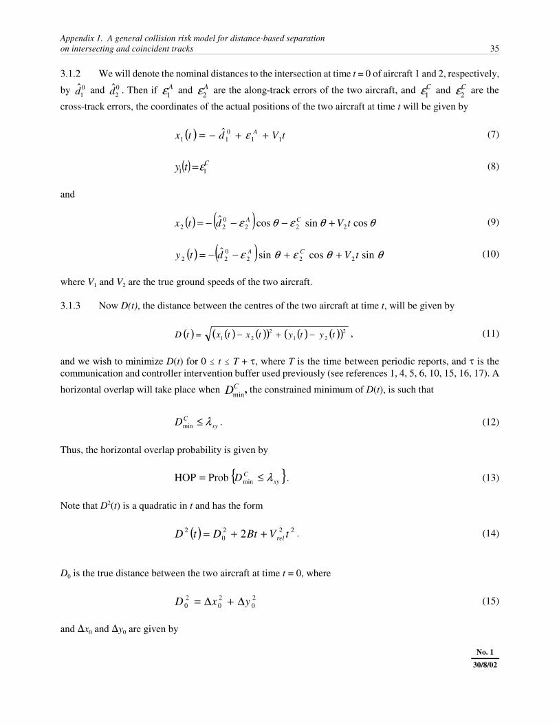
3.1.2 We will denote the nominal distances to the intersection at time t = 0 of aircraft 1 and 2, respectively,
by and . Then if and are the along-track errors of the two aircraft, and and are the01d 0
2d A1ε A
2ε C1ε C
2εcross-track errors, the coordinates of the actual positions of the two aircraft at time t will be given by
(7)( ) tVdtx A11
011
ˆ ++−= ε
(8)( ) Cty 11 ε=
and
(9)( ) ( ) θθεθε cossincosˆ222
022 tVdtx CA +−−−=
(10)( ) ( ) θθεθε sincossinˆ222
022 tVdty CA ++−−=
where V1 and V2 are the true ground speeds of the two aircraft.
3.1.3 Now D(t), the distance between the centres of the two aircraft at time t, will be given by
, (11)( ) ( ) ( )( ) ( ) ( )( )221
221 tytytxtxtD −+−=
and we wish to minimize D(t) for 0 � t � T + �, where T is the time between periodic reports, and � is thecommunication and controller intervention buffer used previously (see references 1, 4, 5, 6, 10, 15, 16, 17). A
horizontal overlap will take place when , the constrained minimum of D(t), is such thatCDmin
. (12)xyCD λ≤min
Thus, the horizontal overlap probability is given by
. (13){ }xyCD λ≤= minProbHOP
Note that D2(t) is a quadratic in t and has the form
. (14)( ) 2220
2 2 tVBtDtD rel++=
D0 is the true distance between the two aircraft at time t = 0, where
(15)20
20
20 yxD ∆+∆=
and �x0 and �y0 are given by

35A Manual on Airspace Planning Methodology for the Determination of Separation Minima
No. 1
30/8/02
(16)( ) ( ) xddxxx εθ +−=−≡∆ 01
02210
ˆcosˆ00
and
. (17)( ) ( ) ydyyy εθ +=−≡∆ sinˆ00 02210
The error terms �x and �y are defined by
(18)θεθεεε sincos 221CAA
x +−=
and
. (19)θεθεεε sincos 221ACC
y −−=
Vrel is the magnitude of the true relative velocity vector, given by
(20)θcos2 21
22
21 VVVVV rel −+=
and B is given by
. (21)( ) θθ sincos 20210 VyVVxB ∆−−∆=
Dmin, the unconstrained minimum of D(t), occurs when
(22)2min relVBtt −==
and after some algebraic manipulation can be written
. (23)( )
relV
VVyVxD
θθ cossin 21020min
−∆+∆=
When � = 0 and V1 = V2, the above needs some special attention because Vrel = 0. In this case the true distancebetween the aircraft is equal to D0 for all t.
3.1.4 If tmin is not in the range 0 to T + �, the constrained minimum of D(t) will be larger than Dmin, andbecause D(t) is a quadratic in t, we have the following:
If tmin < 0 then 0min DDC =
If tmin > T + � then .( )τ+= TDD Cmin

Appendix 1. A general collision risk model for distance-based separationon intersecting and coincident tracks 35B
No. 1
30/8/02
3.1.5 Denoting the nominal ground speeds of the two aircraft by and , we define1V 2V
(24)111 VVv −=
and
. (25)222 VVv −=
3.1.6 Previously (see references 1, 4, 5, 6, 10, 15, 16, 17), we used the “unplanned relative velocity”, v,which is just
. (26)21 vvv −=
This was satisfactory because only coincident tracks (� = 0) were being considered. For the model presentedin this appendix, we require individual speed differences from nominal, so we fitted the data used previouslyfor v by the convolution of two double exponential densities with mean zero and the same scale parameter, �v.In order to keep the ADS model essentially the same as the procedural model, we used the larger of theparameters so obtained, and one obtained by fitting individual aircraft ground speed differences from nominal(obtained from a sample of 10 318 ADS reports during 1994 and 2000). The value chosen was
�v = 5.82 (27)
3.1.7 For computational purposes, we assume , , and are double exponential random variablesA1ε A
2ε C1ε C
2εwith mean zero and scale parameter �n determined from the required navigation performance value. Asindicated above, we also assume that v1 and v2 are double exponential random variables with mean zero andscale parameter �v . Unfortunately, even with these assumptions it is not possible to write down a simplealgebraic form for HOP given in equation 13 except for the relatively simple cases of � = 0 and � = 180°.
3.1.8 Reference 3 proposed a Monte Carlo approach to numerically calculate HOP in the general cases. TheMonte Carlo method used importance sampling and took account of the symmetry of the probability densityfunctions to speed up the computations. Because of the small probabilities involved, it was necessary togenerate a large number of samples when using the Monte Carlo approach. For example, for the longitudinalseparation analyses, the equivalent of approximately 1011 or 100 × 109 samples were used.
3.1.9 One advantage of the Monte Carlo approach is that the correct value of was estimated along withCrelV
the horizontal overlap probability. This was done by assuming that at the point of horizontal overlap the aircrafteach have a random lateral speed, , whose probability density function can be approximated by a doubley�exponential probability density function. The scale parameter of this double exponential density was chosensuch that the convolution of two such densities in the identical track (� = 0) case would produce a value of
, the value that has been used in previous analyses. Note that if the random variable has a probability20=y� y�
density function that is the convolution of two identical double exponential probability density functions with
scale parameter �, then . Thus reference 3 chose23λ=y�
� = 40/3 . (28)

35C Manual on Airspace Planning Methodology for the Determination of Separation Minima
No. 1
30/8/02
3.1.10 An alternative to the Monte Carlo approach is the numerical technique described in reference 18. Theresults presented later in this appendix are based on this numerical technique. Although reference 18 does not
provide a value for , this is not a serious problem in practice. As will be shown below, for � = 0 it isCrelV
possible to derive a theoretical value. This value will suffice for angles smaller that 15 degrees. For larger
angles, Vrel, given by equation 20, will be accurate enough. Note that only enters into the last factor ofCrelV
equation 6, and in general the factor is only slightly larger than unity, so high accuracy is not necessary.
3.2 Same track longitudinal separation
3.2.1 In this case we split the oceanic crossing into m reporting periods of duration T flying hours so thatTC = mT. We assume that the risk of collision in each reporting interval is the same so that the total risk is justm times the risk of collision in any one interval. Assuming the two aircraft are at the same nominal level,equation 6 can be written
(29)( ) ( )��
�
�
��
�
�⋅+××+×=
Crel
xy
zz
V
zPT
T 2210HOP
2CR
πλλ
τ�
where HOP(T + �) is the horizontal overlap during a time equal to one reporting period plus the communicationand controller intervention buffer � used previously (see references 1, 4, 5, 6, 10, 15, 16, 17), and we have usedNP = 1/TC = 1/mT. If two aircraft have significantly different nominal speeds, the assumption that the total riskfor the oceanic crossing will be m times that for one reporting period will be somewhat pessimistic because theaircraft may only constitute a pair for less than m reporting periods.
3.2.2 When the numerical calculations indicate that the risk is largest for � = 0, then it will be more accurateto use the following good approximation to the horizontal overlap probability HOP. By taking � = 0 inequations 7, 8, 9 and 10, we can obtain
(30)( ) ( ) ( ) tVVddtxtx AA2121
01
0221
ˆˆ −+−+−=− εε
and
. (31)( ) ( ) CCtyty 2121 εε −=−
3.2.3 Treating the x and y directions independently and taking t = T + �, since it maximizes the risk in thiscase, we can approximate the horizontal overlap probability by the product of the probability the aircraft arein longitudinal overlap or out of order at time t = T + � and the lateral overlap probability. Thus
(32)( )0LOPHOP yP×=
where Py(0) is the lateral overlap probability of two aircraft with wingspan �y = �xy, which are nominally on thesame (identical) track, and the longitudinal overlap probability, LOP, is given by

Appendix 1. A general collision risk model for distance-based separationon intersecting and coincident tracks 35D
No. 1
30/8/02
. (33)( ) ( ){ }xyTxTx λττ ≤+−+≈ 21ProbLOP
The approximation is quite good unless T + � is significantly smaller than the values used in section 4.
3.2.4 The nominal longitudinal separation at time t = T + � is given by
, (34)( )( )τ+−+−= TVVddS 2101
02
ˆˆˆˆˆ
so
. (35)( ) ( ) ( )( )τεεττ +−+−+=+−+ TvvSTxTx AA212121
ˆ
3.2.5 Using this result in equation 33 and carrying out the convolution involved, assuming the distribution
of is uniform between the limits A and B, where B is very much larger than A, we obtain:S
(36)( ) ( )��
�
��
��
���
����
� −−+��
�
����
� −−
≈2
222
21 exp1exp
41
LOPλ
λβλ
λλ
βλA
SA
SAB
xy
n
xyn
where
�n = RNP/2.995732, (37)
�2 = �v × (T + �), (38)
, (39)( )22
22 λλλβ −= nn
, (40)( )βλ
λ−++
−= 1431
n
xyAS
and
. (41)βλ
λ43
22 ++
−= xyA
S
Note that, in general, the nominal longitudinal separation at time t is given by
(42)( ) ( ) ( )tdtdtS 12ˆˆˆ −=
where and are the nominal distances to the intersection at time t, given by( )td1ˆ ( )td2
ˆ
35E Manual on Airspace Planning Methodology for the Determination of Separation Minima
No. 1
30/8/02
(43)( ) tVdtd 10
11ˆˆˆ +=
and
. (44)( ) tVdtd 2022
ˆˆˆ +=
3.2.6 We assume that if , the controller will increase the separation between the aircraft at time t = 012ˆˆ VV >
if necessary to ensure that the aircraft will still be correctly separated after time T + �. If, on the other hand,, the leading aircraft is nominally faster than the trailing one, and the risk of collision will be substantially12
ˆˆ VV <reduced. For these reasons, as well as the one stated above concerning the sum of the risks in each reportinginterval, for calculation purposes we will conservatively assume that the nominal speeds of the two aircraft arethe same. For computational purposes, we also assume that is a random variable whose probability density( )0S
function is a uniform density between the distance-based longitudinal separation minimum Sx and Sx + 250(nautical miles). When � = 0 this implies that A = Sx and B = Sx + 250.
3.2.7 As mentioned previously, when � = 0 it is also possible to derive a mathematical expression for .CrelV
By definition
(45)( )
τλ
+≤+
=T
wswV xyC
rel
|E
where E denotes the expected value, , and as in equation 26. TheAASs 21ˆ εε −+= ( )τ+= Tvw 21 vvv −=
conditional density of w is given by
(46)( ) ( ) ( ) LOP| wHwgwswg xyxy −=≤+ λλ
where
, (47)( ) ( ) ( )1exp4
122
2
+⋅−= λλλ
wwwg
and
(48)( ) ( )
( )��
�
��
�
<<<���
����
�+−⋅��
�
����
� −−
+−−
≤���
����
�+−⋅��
�
����
� −−
=.for ,3exp
4
for ,3exp4
11
1
11
1
BsAAssA
ABABAs
AssAAs
ABsH
λλλ
λλλ
Appendix 1. A general collision risk model for distance-based separationon intersecting and coincident tracks 35F
No. 1
30/8/02
Therefore
, (49)( ) ( ) ( ) LOPd ⋅+−≈ �∞
−=τλ TvvHvvgV xy
Mv
Crel
where M satisfies A << M << B.
3.2.8 Although it is possible to write down an analytical expression for , the expression is quiteCrelV
complicated. A simpler approach that is accurate enough for this purpose is to use numerical integration withM = Sx + 50. We also replace the upper integral limit by zero since the contribution from positive v values isnegligible. Typical values obtained using this expression are given in section 4.
3.3 Reciprocal track longitudinal separation for ADS
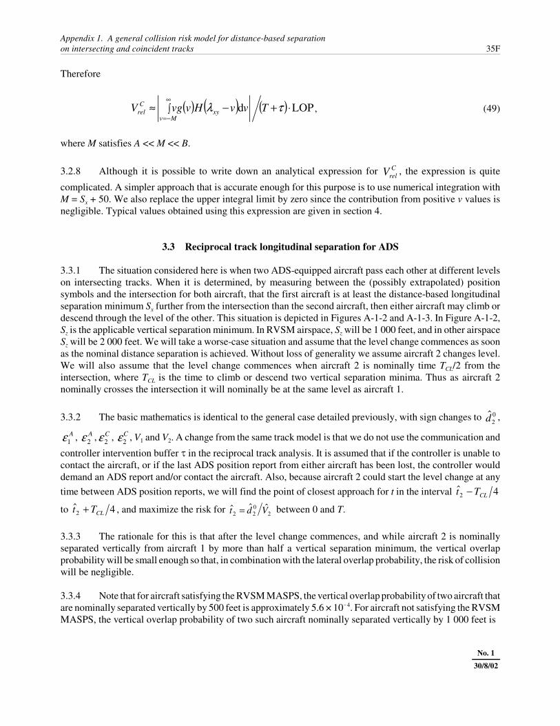
3.3.1 The situation considered here is when two ADS-equipped aircraft pass each other at different levelson intersecting tracks. When it is determined, by measuring between the (possibly extrapolated) positionsymbols and the intersection for both aircraft, that the first aircraft is at least the distance-based longitudinalseparation minimum Sx further from the intersection than the second aircraft, then either aircraft may climb ordescend through the level of the other. This situation is depicted in Figures A-1-2 and A-1-3. In Figure A-1-2,Sz is the applicable vertical separation minimum. In RVSM airspace, Sz will be 1 000 feet, and in other airspaceSz will be 2 000 feet. We will take a worse-case situation and assume that the level change commences as soonas the nominal distance separation is achieved. Without loss of generality we assume aircraft 2 changes level.We will also assume that the level change commences when aircraft 2 is nominally time TCL/2 from theintersection, where TCL is the time to climb or descend two vertical separation minima. Thus as aircraft 2nominally crosses the intersection it will nominally be at the same level as aircraft 1.
3.3.2 The basic mathematics is identical to the general case detailed previously, with sign changes to ,02d
, , , , V1 and V2. A change from the same track model is that we do not use the communication andA1ε A
2ε C2ε C
2εcontroller intervention buffer � in the reciprocal track analysis. It is assumed that if the controller is unable tocontact the aircraft, or if the last ADS position report from either aircraft has been lost, the controller woulddemand an ADS report and/or contact the aircraft. Also, because aircraft 2 could start the level change at anytime between ADS position reports, we will find the point of closest approach for t in the interval 42 CLTt −
to , and maximize the risk for between 0 and T.42 CLTt + 2022
ˆˆˆ Vdt =
3.3.3 The rationale for this is that after the level change commences, and while aircraft 2 is nominallyseparated vertically from aircraft 1 by more than half a vertical separation minimum, the vertical overlapprobability will be small enough so that, in combination with the lateral overlap probability, the risk of collisionwill be negligible.
3.3.4 Note that for aircraft satisfying the RVSM MASPS, the vertical overlap probability of two aircraft thatare nominally separated vertically by 500 feet is approximately 5.6 × 10�4. For aircraft not satisfying the RVSMMASPS, the vertical overlap probability of two such aircraft nominally separated vertically by 1 000 feet is

35G Manual on Airspace Planning Methodology for the Determination of Separation Minima
No. 1
30/8/02
S
S
S
S
S
z
x
z
z
z
1
2
Figure A-1-2. Side view of the reciprocal track scenario
x
y
Actual position of aircraft 1
Actual position of aircraft 2Nominal position of aircraft 1
Nominal position of aircraft 2
Figure A-1-3. Nominal and actual positions of aircraftat time t = 0 (reciprocal tracks)

Appendix 1. A general collision risk model for distance-based separationon intersecting and coincident tracks 35H
No. 1
30/8/02
approximately 9.3 × 10�6. These values are based on modelling the vertical errors by Gaussian-doubleexponential mix densities as in reference 8. In the calculations we use Pz(0) for the vertical overlap probabilitybecause the actual nominal vertical separation when a horizontal overlap occurs is not known, and as explainedin section 2, Pz(0) gives an overestimate of the collision risk.
3.3.5 A further change from the same track model is that instead of assuming the initial separation betweenthe aircraft is a random variable with a uniform probability density, as in the previous section, we assume, asmentioned above, that the second aircraft will commence its level change as soon as the first aircraft is thelongitudinal separation minimum Sx further from the intersection than the second aircraft (and getting furtheraway).
3.3.6 The final item that requires some discussion is the value of NP, the number of pairs per flight hour.For longitudinal distance-based separation, as explained above, the appropriate value is 1/T. We will assumefor the type of procedure that we are analysing here that aircraft would not be changing levels in this mannermore frequently than once every reporting period and hence use the same factor, although this is almostcertainly overly pessimistic. The collision risk equation in this case is then the same as equation 29, with thechanges mentioned above.
3.3.7 If, as indeed will turn out to be the case, the risk is maximized for � = 180°, then it is possible toproduce a good approximation to the horizontal overlap probability HOP in a similar manner as we did
previously for � = 0. By taking � = 180° and changing the sign of in equations 7, 8, 9 and 10, we can obtain01d
(50)( ) ( ) ( ) tVVddtxtx AA2121
02
0121
ˆˆ ++++−=− εε
and
. (51)( ) ( ) CCtyty 2121 εε +=−
3.3.8 Treating the x and y directions independently, and taking since it maximizes the risk in this,2 Tt =case, we can approximate the horizontal overlap probability by the product of the probability the aircraft arein longitudinal overlap or out of order at time T � TCL/4 and the lateral overlap probability Py(0). Thus
. (52)( ) ( ){ } ( )0P44ProbHOP 12 yxyCLCL TTxTTx ×≤−−−≈ λ
3.3.9 The nominal longitudinal separation at time T � TCL/4 is given by
, (53)( )21ˆˆ
4ˆ VV
TSS CL
x ++=
so
. (54)( ) ( ) ( )( )4ˆ44 212121 CLAA
CLCL TTvvSTTxTTx −++++=−−− εε

35I Manual on Airspace Planning Methodology for the Determination of Separation Minima
No. 1
30/8/02
3.3.10 Using this result in equation 52 and carrying out the convolution involved in the longitudinal overlapterm, we obtain
, (55)( ) ( )
��
�
��
��
��
�
�
��
�
� +−−+
��
�
�
��
�
� +−=
2
22
21
ˆexp1
ˆexp
4
0HOP
λλ
βλ
λβ xy
n
xyy SS
SS
P
where,
�n, = RNP/2.995732, (56)
�2 = �v,× (T � TCL/4), (57)
, (58)( )22
22 λλλβ −= nn
, (59)( )βλ
λ−++
−= 142
ˆ1
n
xySS
and
. (60)βλ
λ42
ˆ
22 ++
−= xyS
S
3.4 Lateral separation on intersecting tracks
3.4.1 Several versions of a mathematical methodology applicable to intersecting tracks have been presentedpreviously (see references 2, 7 and 9). Considerable debate has taken place as to the validity of thosemethodologies. As a result of that debate the present methodology is based on the more robust methodologypresented in section 3.1.
3.4.2 Lateral separation of aircraft on intersecting tracks is based on the concept of a defined area of conflictaround the intersection. The area of conflict is a quadrilateral (see Figure A-1-4), the corners of which areknown as lateral separation points, defined as the points on a track where the perpendicular distance to the othertrack is equal to the lateral separation minimum, which we will denote Sy. Lateral separation is achieved by thecontroller ensuring that two aircraft will not be simultaneously within the area of conflict at the same level.
3.4.3 Suppose two aircraft are both approaching the intersection as in Figure A-1-5. We will assume thataircraft 1 will (nominally) get to the intersection first. A distance-based procedure for ensuring the aircraft arelaterally separated is for the controller to ask both pilots for distances to the intersection before it is estimatedthat the second aircraft will get within, say, half a longitudinal separation minimum of the lateral separationpoint it is approaching. As with longitudinal separation, in a procedural environment, the controller shouldensure an underestimate of the nominal separation by ensuring the leading aircraft responds first.

Appendix 1. A general collision risk model for distance-based separationon intersecting and coincident tracks 35J
No. 1
30/8/02
Sy
S y
LEGEND
Lateral separation points
Area of conflict
Figure A-1-4. Lateral separation points and the area of conflict
3.4.4 In an ADS environment the estimates may be based on (possibly extrapolated) position information.Based on reported or calculated distances to the intersection, the nominal ground speeds of the two aircraft, and
the known reporting time, the controller calculates , the time of entry of aircraft 2 into the area of conflict,Et2
and and , the times of entry and exit of aircraft 1 to and from the area of conflict. If , thenEt1Lt1
LEE ttt 121 ≤≤the aircraft will be simultaneously in the area of conflict at some time, and so aircraft 2 will be required to beat a vertically separated level by the lateral separation point. Note that some States, for example Australia,require the second aircraft to be at a vertically separated level by distance Sx /2 from the lateral separation point,or, equivalently, by distance from the intersection, where , the distance of the lateral separation point2xS+� �
from the intersection, is determined from
. (61)θsinyS=�
3.4.5 This appendix, however, does not use this extra requirement, assuming only that the aircraft will notbe permitted to be simultaneously in the area of conflict at the same level. The results presented in section 4indicate that the target level of safety will be met without it.

35K Manual on Airspace Planning Methodology for the Determination of Separation Minima
No. 1
30/8/02
1
2
Figure A-1-5. Both aircraft approaching the area of conflict
3.4.6 There are two different cases to deal with here:
a) Both aircraft approaching the area of conflict. For the analysis of this situation, we will take asa worse case that both aircraft have equal nominal speeds and are nominally as close as possibleafter time T + �. Thus we assume that at time t = 0 that
(62)( )τ++= TVd 101
ˆˆ �
and
. (63)01
02
ˆˆ dd =
Because the aircraft could report at any time prior to entering the area of conflict, we take themaximum risk value with respect to T. Note that, in reality, aircraft 2 would be required to be ata vertically separated level by distance from the intersection, but we conservatively assume that�
it is at the same level as aircraft 1 until it is distance from the intersection and then is�
instantaneously at a vertically separated level. The situation is shown in Figure A-1-5. Theanalysis of this situation is similar to that for longitudinal separation, except that the nominal

Appendix 1. A general collision risk model for distance-based separationon intersecting and coincident tracks 35L
No. 1
30/8/02
1
2
Figure A-1-6. One aircraft leaving the area of conflict as another is entering
distances of the aircraft to the intersection at time t = 0 are different. The value of NP in the basiccollision risk model also needs some discussion here. The worse case would be that every aircrafton one track is paired with an aircraft on the other track. Clearly they could be, but not all pairswould then be at the minimum separation considered for this analysis. In fact, on average, thedifference in nominal distances of the pairs to the intersection would be at least Sx/2. Further, aspointed out in section 2, in practice NP is often significantly smaller than 1.
b) One aircraft leaving the area of conflict as another is entering. This situation is depicted inFigure A-1-6. The analysis is the same as for the basic case, but, of course, the nominal separationis different. As a worse case we will assume both aircraft are nominally at the same level and thataircraft 1 is nominally leaving the area of conflict as aircraft 2 is entering. Thus, we take
(64)TVd 101
ˆˆ =
and
. (65)( )12202
ˆˆ1ˆˆ VVTVd +×+= �

35M Manual on Airspace Planning Methodology for the Determination of Separation Minima
No. 1
30/8/02
To maximize the risk over all possible reporting times, we assume the aircraft report when aircraft1 is time T before the intersection, and we maximize the risk over two reporting periods. Note thatwhen the angle of intersection is 45 (or 135) degrees, it typically takes less than 20 minutes foran aircraft to traverse the area of conflict when the lateral separation minimum is 50 NM, and lessthan 11 minutes when the lateral minimum is 30 NM.
4. RESULTS
4.1 General
4.1.1 The results in this appendix were computed under essentially the same assumptions as for references4, 8, 9 and 10, except for the following:
a) The Mach number technique is no longer assumed, although obviously controllers will still applyspeed control to aircraft if required. Individual aircraft speed uncertainty is assumed to follow adouble exponential probability density function, as explained in section 3.1.
b) Aircraft are assumed to be cylinders of diameter �xy and �z height. RNP 10 aircraft will beassumed to be of diameter 192.2 feet and height 54.8 feet, whereas RNP 4 aircraft will beassumed to be of diameter 231.8 feet and height 63.4 feet.
c) Because of the widespread use of RVSM, the assumed value of Pz(0) has been increased to 0.48for RNP 10 aircraft and 0.55 for RNP 4 aircraft.
d) The equivalent of and , namely is used in the calculations. As noted above, in generalx� y� CrelV
the value depends on the separation minimum in use, the value of T + � , the RNP value of theaircraft, as well as the angle between the tracks of the two aircraft. When the risk is largest at� = 0, we use the theoretical value given by equation 49. Typical values are presented inTable A-1-1 for RNP 4. When � is close to zero (less than 15 degrees) we use the values inTable A-1-1. When � is not close to zero, sufficient accuracy may be obtained by using theunconditional relative velocity, i.e.
(66)θcos2 212
22
1 VVVVV Crel −+=
Table A-1-1. values for ���� = 0, RNP4CrelV
T = 32 min, Sx = 50 NM T = 14 min, Sx = 30 NM
� = 4 min 91.9 kt 87.7 kt
� = 10.5 min 80.5 kt 76.6 kt
� = 13.5 min 76.2 kt 71.1 kt
Appendix 1. A general collision risk model for distance-based separationon intersecting and coincident tracks 35N
No. 1
30/8/02
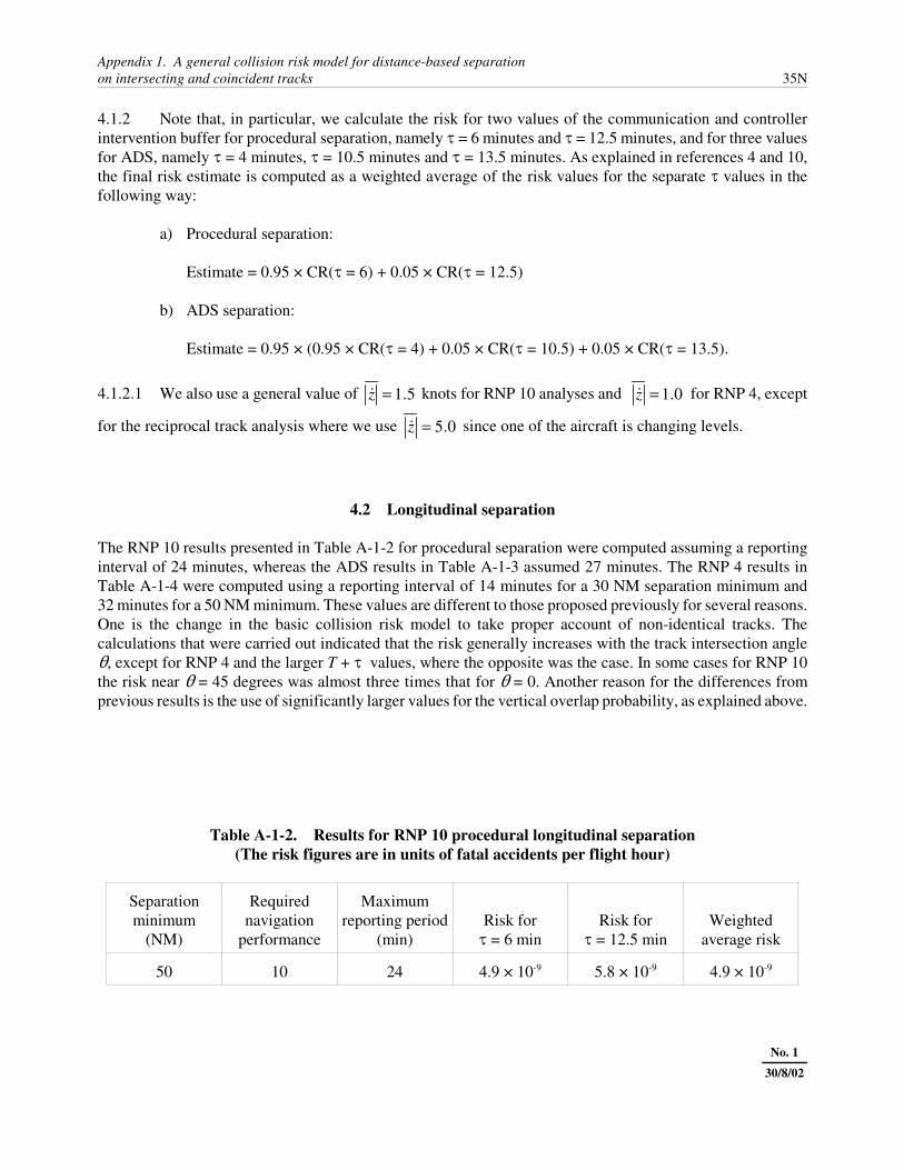
4.1.2 Note that, in particular, we calculate the risk for two values of the communication and controllerintervention buffer for procedural separation, namely � = 6 minutes and � = 12.5 minutes, and for three valuesfor ADS, namely � = 4 minutes, � = 10.5 minutes and � = 13.5 minutes. As explained in references 4 and 10,the final risk estimate is computed as a weighted average of the risk values for the separate � values in thefollowing way:
a) Procedural separation:
Estimate = 0.95 × CR(� = 6) + 0.05 × CR(� = 12.5)
b) ADS separation:
Estimate = 0.95 × (0.95 × CR(� = 4) + 0.05 × CR(� = 10.5) + 0.05 × CR(� = 13.5).
4.1.2.1 We also use a general value of knots for RNP 10 analyses and for RNP 4, except5.1=z� 0.1=z�
for the reciprocal track analysis where we use since one of the aircraft is changing levels.0.5=z�
4.2 Longitudinal separation
The RNP 10 results presented in Table A-1-2 for procedural separation were computed assuming a reportinginterval of 24 minutes, whereas the ADS results in Table A-1-3 assumed 27 minutes. The RNP 4 results inTable A-1-4 were computed using a reporting interval of 14 minutes for a 30 NM separation minimum and32 minutes for a 50 NM minimum. These values are different to those proposed previously for several reasons.One is the change in the basic collision risk model to take proper account of non-identical tracks. Thecalculations that were carried out indicated that the risk generally increases with the track intersection angle�, except for RNP 4 and the larger T + � values, where the opposite was the case. In some cases for RNP 10the risk near � = 45 degrees was almost three times that for � = 0. Another reason for the differences fromprevious results is the use of significantly larger values for the vertical overlap probability, as explained above.
Table A-1-2. Results for RNP 10 procedural longitudinal separation(The risk figures are in units of fatal accidents per flight hour)
Separationminimum
(NM)
Requirednavigation
performance
Maximumreporting period
(min)Risk for� = 6 min
Risk for� = 12.5 min
Weightedaverage risk
50 10 24 4.9 × 10⁻⁹ 5.8 × 10⁻⁹ 4.9 × 10⁻⁹

35O Manual on Airspace Planning Methodology for the Determination of Separation Minima
No. 1
30/8/02
Table A-1-3. Results for RNP 10 ADS separation(The risk figures are in units of fatal accidents per flight hour)
Separationminimum
(NM)
Requirednavigation
performance
Maximumreporting period
(min)Risk for� = 4 min
Risk for� = 10.5 min
Risk for� = 13.5 min
Weightedaverage risk
50 10 27 4.0 × 10⁻⁹ 8.2 × 10⁻⁹ 8.2 × 10⁻⁹ 4.4 × 10⁻⁹
Table A-1-4. Results for RNP 4 ADS separation(The risk figures are in units of fatal accidents per flight hour)
Separationminimum
(NM)
Requirednavigation
performance
Maximumreporting period
(min)Risk for� = 4 min
Risk for� = 10.5 min
Risk for� = 13.5 min
Weightedaverage risk
30 4 14 3.6 × 10⁻¹⁰ 1.6 × 10⁻⁸ 5.7 × 10⁻⁸ 3.9 × 10⁻⁹
50 4 32 1.4 × 10⁻⁹ 1.3 × 10⁻⁸ 2.8 × 10⁻⁸ 3.3 × 10⁻⁹
Table A-1-5. Results for ADS reciprocal track longitudinal separation(The risk figures are in units of fatal accidents per flight hour)
Requirednavigation
performance
Longitudinalseparation
minimum (NM)
Verticalseparation
minimum (ft)Maximum ADS
reporting period (min)Time to change
level (min) Risk estimate
10 50 2 000 27 8 1.7 × 10⁻¹⁰
10 50 1 000 27 4 3.2 × 10⁻⁹
4 30 2 000 14 8 3.9 × 10⁻¹⁶
4 30 1 000 14 4 1.1 × 10⁻¹²
4.3 Reciprocal track longitudinal separation for ADS
As mentioned in section 3.3, it turns out that the risk for this case was maximized at � = 180°. Therefore wecan use the results based on the analytical formula given in equation 55. The results are presented inTable A-1-4. Again, the RNP 10 results use a vertical overlap probability of 0.48 and the RNP 4 results use a

Appendix 1. A general collision risk model for distance-based separationon intersecting and coincident tracks 35P
No. 1
30/8/02
value of 0.55. Also, because one aircraft is changing levels we use a value of 5 knots. This is approximatelyz�
500 feet per minute, a typical climb performance. The figures quoted in Table A-1-5 are for nominal aircraftspeeds of 300 knots because that gives the largest risk values, although it is most unlikely that both aircraftwould have ground speeds this slow if they were on reciprocal tracks. The results were calculated for onereporting period for each RNP value because, the larger the reporting period, the larger the risk due to the largerextrapolation errors. It was also assumed that in RVSM airspace the level change would take 4 minutes, andin conventional airspace this would take 8 minutes.
4.4 Lateral separation
The results for both parts of this section have been calculated assuming a value for NP, the number of pairs perflight hour, of 0.5. An analysis of aircraft reporting times at intersections in the Tasman Sea area, based on bothhistorical data from 1993 and 1994, as well as simulated data based on six weeks of flight plans from 1998 and1999, gives an NP value of approximately 0.02 over all intersections. Thus the results presented should beconservative by a factor of approximately 25 for the Tasman and therefore should also be applicable to airspacethat has significantly more traffic than the Tasman. Note that the NP factor allows for aircraft that take part inmultiple pairings at various intersections as they traverse the airspace. Note also that all pairs are assumed tobe at minimum separation. This again is somewhat conservative.
a) Both aircraft entering the area of conflict. The results based on the methodology of reference 18are given in Table A-1-6. Computations were carried out for angles between 15 and 135 degrees.The risk was largest at � = 15 degrees.
b) One aircraft entering the area of conflict as another is leaving. The results given in Table A-1-7were computed using a variety of combinations of aircraft speeds as shown. Calculations werecarried out for angles between 15 and 135 degrees. For RNP 10 the risk was maximized at� = 135 degrees in all cases; however this was not always the case for RNP 4.
Table A-1-6. Results for lateral separation of aircraft on intersecting tracks,where both aircraft are approaching the area of conflict
(The risk figures are in units of fatal accidents per flight hour)
Requirednavigation
performance
Lateralseparation
minimum (NM)
Maximumreporting period
(min) Estimated risk
10 50 24 1.1 × 10⁻⁹
10 50 27 1.1 × 10⁻⁹
4 30 14 4.4 × 10⁻¹³

35Q Manual on Airspace Planning Methodology for the Determination of Separation Minima
No. 1
30/8/02
Table A-1-7. Results for lateral separation of aircraft on intersecting tracks,where one aircraft is entering area of conflict while another is leaving
(The risk figures are in units of fatal accidents per flight hour)
Requirednavigation
performance
Lateralseparation
minimum (NM)
Maximumreporting period
(min)Nominal speed offirst aircraft (kt)
Nominal speedof secondaircraft
(kt) Estimated risk
10 50 27 300 600 2.4 × 10⁻⁹
10 50 27 480 480 1.4 × 10⁻⁹
10 50 27 300 300 1.7 × 10⁻⁹
10 50 27 600 300 1.6 × 10⁻⁹
4 30 14 300 600 6.4 × 10⁻¹¹
4 30 14 480 480 3.0 × 10⁻¹¹
4 30 14 300 300 2.2 × 10⁻¹²
4 30 14 600 300 3.6 × 10⁻¹³
5. ACKNOWLEDGEMENTS
The author is indebted to Karim Mehadhebi for the numerical technique described in reference 18 and also forproviding the related software that was used to perform the numerical calculations in this appendix. The authorwould also like to thank the members of the RGCSP Mathematicians Subgroup for many valuable commentsand suggestions that have improved the presentation.
6. REFERENCES
1. Anderson, D. and Karppinen, N.E., A Collision Risk Analysis of Data from the Oakland and Pacific Areas,ICAO RGCSP WG/A WP/15, September 1994.
2. Anderson, David, A Collision Risk Analysis of Intersecting Tracks, ICAO RGCSP WG/A WP/7,April 1998.
3. Anderson, David, A General Collision Risk Model for Distance-Based Separation on Intersecting andCoincident Tracks, ICAO RGCSP WG/A WP/12 (revised), November 2000.
4. Anderson, David, An Extended Methodology for ADS Longitudinal Separation Standards, ICAORGCSP/10 WP/7, May 2000.
5. Anderson, D., Details of Derivations in WP9 (Seattle) and WP15, WP9 (Singapore), unpublished workingpaper, 1994.

Appendix 1. A general collision risk model for distance-based separationon intersecting and coincident tracks 35R
No. 1
30/8/02
6. Anderson, D., On the Standard Longitudinal Collision Risk Equation, RGCSP/9 WP/7, May 1996.
7. Anderson, D. and Lin, X.G., A Collision Risk Model for a Crossing Track Separation Methodology, ICAORGCSP/9 WP/9, May 1996.
8. Anderson, D. and Lin, X.G., A Methodology for ADS Reciprocal Track Longitudinal SeparationStandards, ICAO RGCSP/10 WP/21, May 2000.
9. Anderson, D. and Lin, X.G., A Modified Collision Risk Model for a Crossing Track SeparationMethodology, ICAO RGCSP/10 WP/14, May 2000.
10. Anderson, D. and Lin, X.G., An Extended Methodology for Longitudinal Same-Track Separation, ICAORGCSP/10 WP/9, May 2000.
11. Brooker, P. and Lloyd, D.E., Collision Risk and Longitudinal Separation Standards for North Atlantic AirTraffic, DORA communication 7801, Civil Aviation Authority, London, 1978.
12. Flax, B., Estimating the Probability and Duration of Horizontal Overlaps Experienced by AirplanesAssigned to the Same Flight Level on Intersecting Oceanic Routes, ICAO RGCSP WG/A WP/2,May 1999.
13. Flax, B., Estimating the Rate of Collisions Between Airplanes Assigned to the Same Flight Level onIntersecting Oceanic Routes, ICAO RGCSP WG/A WP/3, May 1999.
14. ICAO Doc 4444, Procedures for Air Navigation Services, Rules of the Air and Air Traffic Services,Thirteenth Edition, 1996.
15. ICAO Doc 9689-AN/953, Manual on Airspace Planning Methodology for the Determination ofSeparation Minima, First Edition, 1998.
16. Karppinen, N.E. and Anderson, D., A General Methodology Relating Navigational Performance toLongitudinal Distance Separation, ICAO RGCSP WG/A WP/9, September 1993.
17. Karppinen, N.E. and Anderson, D., A Preliminary Collision Risk Analysis Using Data from the PacificArea, ICAO RGCSP WG/A WP/8 September 1993.
18. Mehadhebi, K., Analytical Derivation of the Crossing Track ADS Model, CENA/NT01-508, 9 January 2001.
19. Reich, PG. Analysis of Long-Range Air Traffic Systems — Separation Standards I, Journal of Navigation,1966.
20. Reich, PG. Analysis of Long-Range Air Traffic Systems — Separation Standards II, Journal of Navigation,1966.
21. Reich, PG. Analysis of Long-Range Air Traffic Systems — Separation Standards III, Journal ofNavigation, 1966.


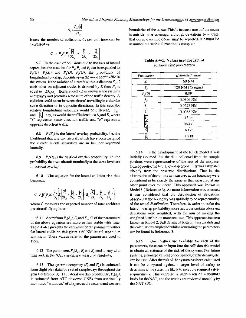


60 Manual on Airspace Planning Methodology for the Determination of Separation Minima
REFERENCES
1. A General Methodology Relating NavigationalPerformance to Longitudinal Distance Separation.Karppinen, N.E. and Anderson, D., ICAO RGCSPWG/A WP/9, September 1993.
2. A preliminary collision risk analysis using datafrom the Pacific Area. Karppinen, N.E. andAnderson, D., ICAO RGCSP WG/A WP/8,September 1993.
3. A Collision Risk Analysis Relating NavigationalPerformance to Initial ADS LongitudinalSeparation Minima Using the FANS 1 AvionicsPackage. Anderson, D. and Karppinen, N.E.,ICAO RGCSP WG/A WP/9, May 1994.
4. A Collision Risk Analysis Relating NavigationalPerformance to Initial ADS LongitudinalSeparation Minima For Initial ARINC 622 ADSImplementations. Anderson, D. and Karppinen,N.E., ICAO RGCSP WG/A WP/10, September1994.
5. A Collision Risk Analysis of Data from theOakland and Pacific Areas. Anderson, D. and
Karppinen, N.E., ICAO RGCSP WG/A WP/15,September 1994.
6. Reich, P.G., Analysis of Long-Range Air TrafficSystems — Separation Standards I. Journal of theInstitute of Navigation, 1966.
7. Reich, P.G., Analysis of Long-Range Air TrafficSystems — Separation Standards II. Journal of theInstitute of Navigation, 1966.
8. Reich, P.G., Analysis of Long-Range Air TrafficSystems — Separation Standards III. Journal ofthe Institute of Navigation, 1966.
9. Air Traffic Services System Requirements andObjective (Draft Rev E). Boeing CommercialAirplane Group, Document No. D240U123.
10. Price, F., A Minimum Rate of Position Reportingfor Automatic Dependant Surveillance. ICAOADSP/2 WP/28, June 1992.
11. Price, F., Position Data Refresh in AutomaticDependent Surveillance. ICAO ADSP/2 WP/27,June 1992.
No. 1
30/8/02
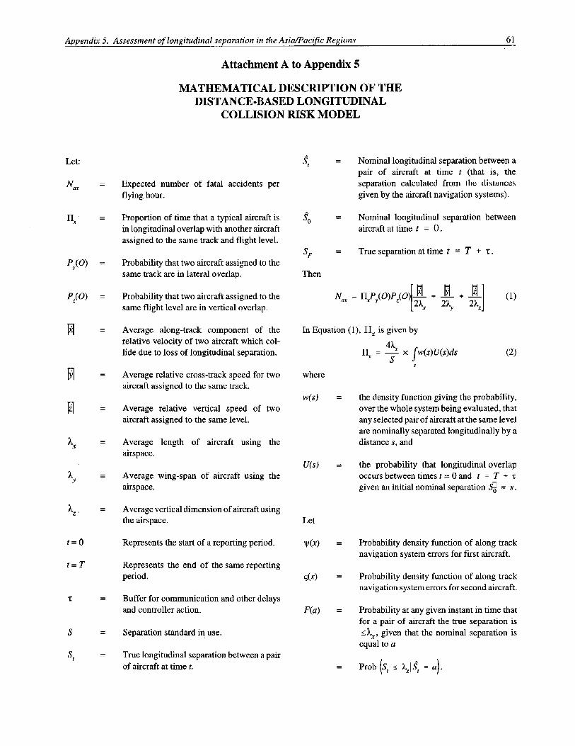


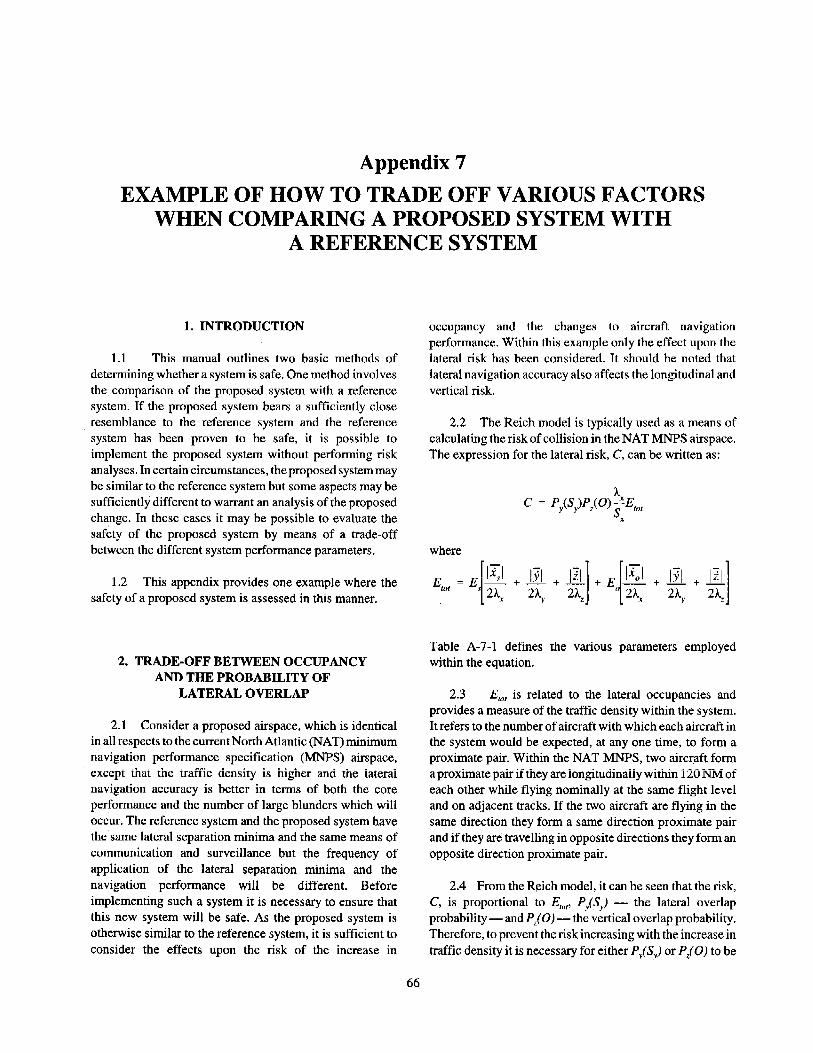
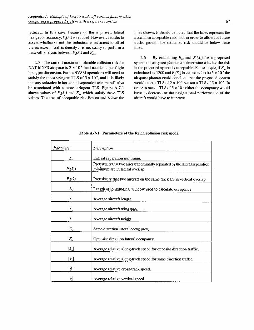


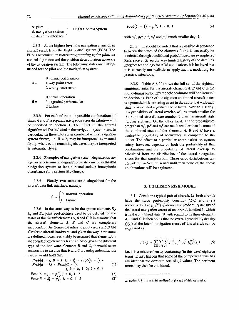

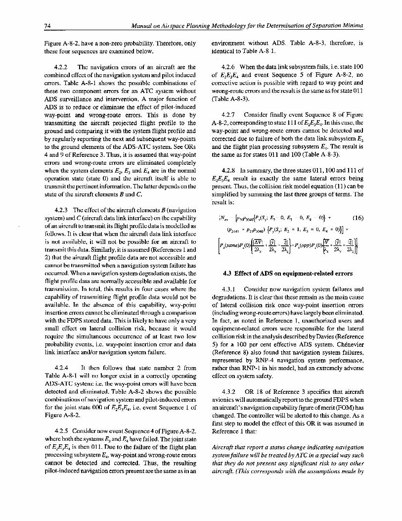

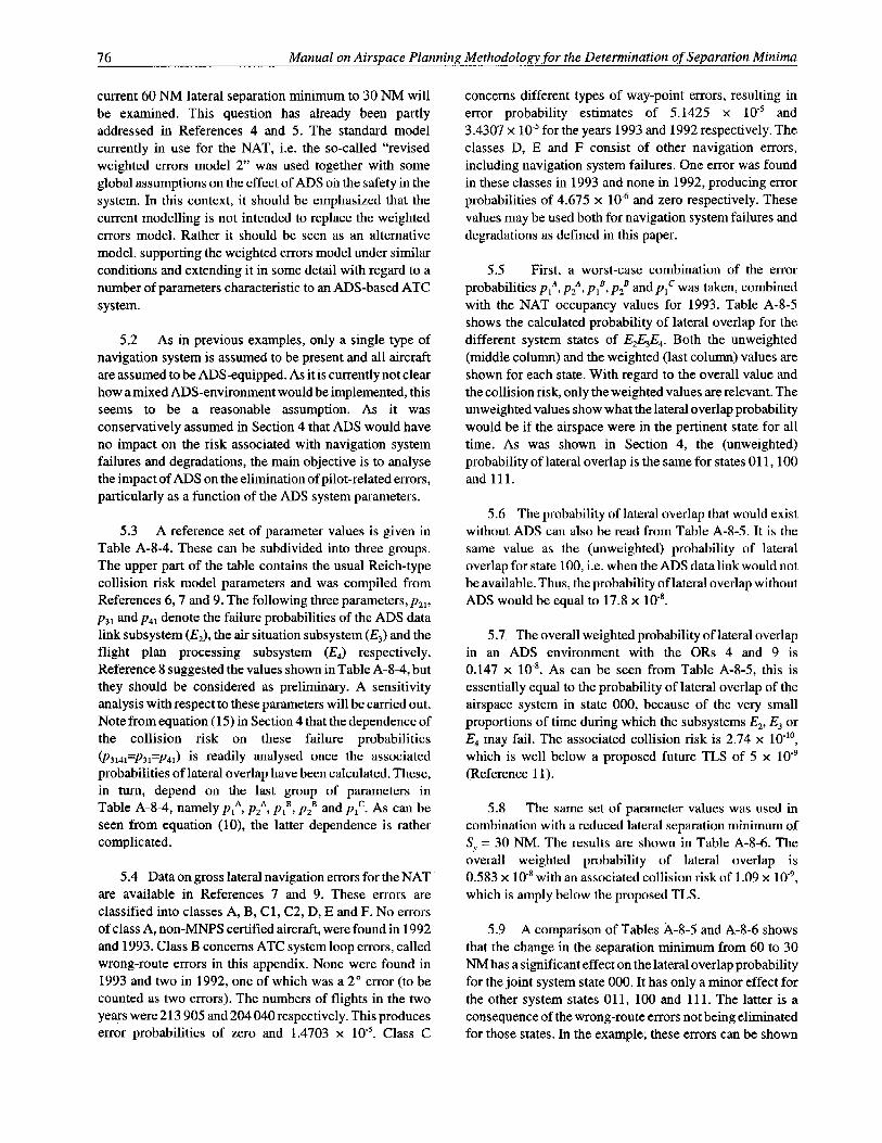


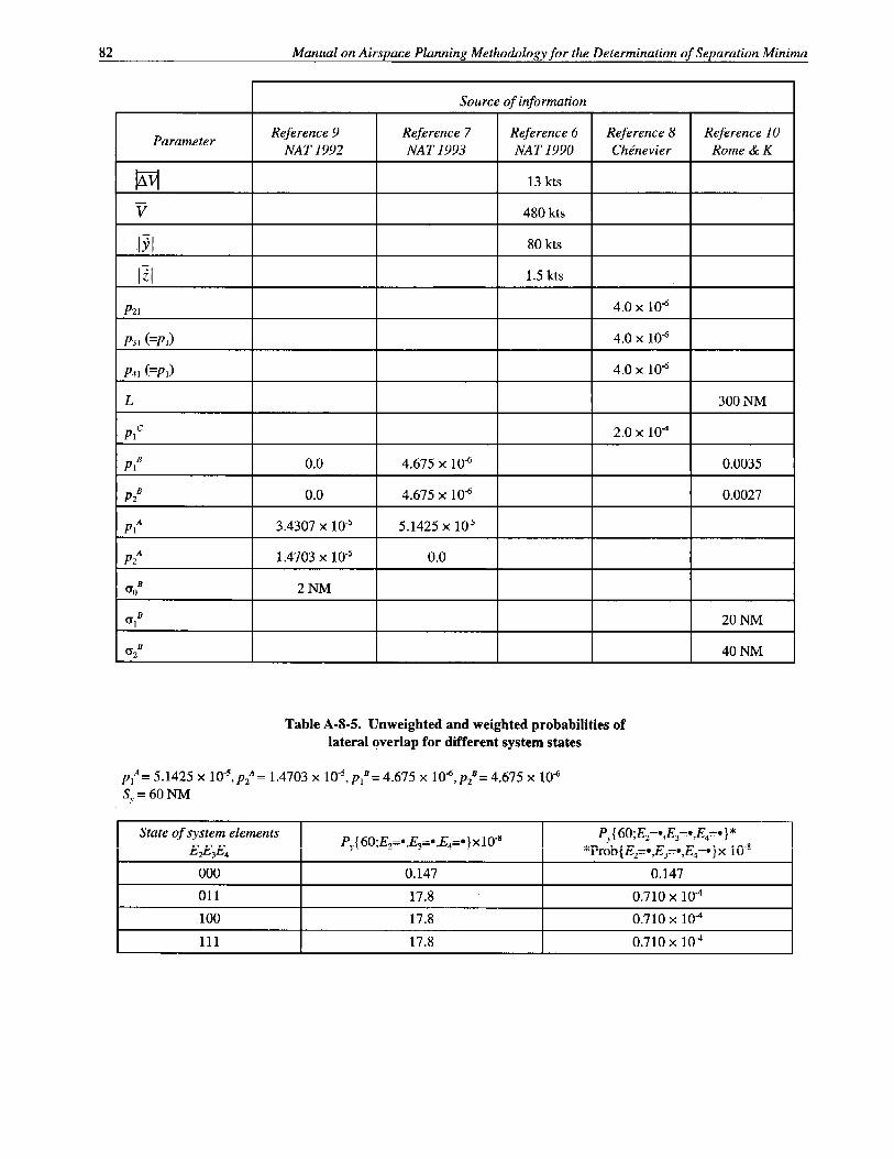


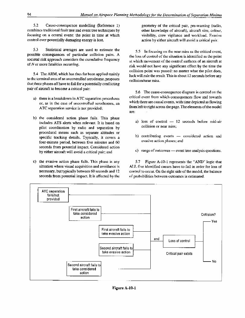
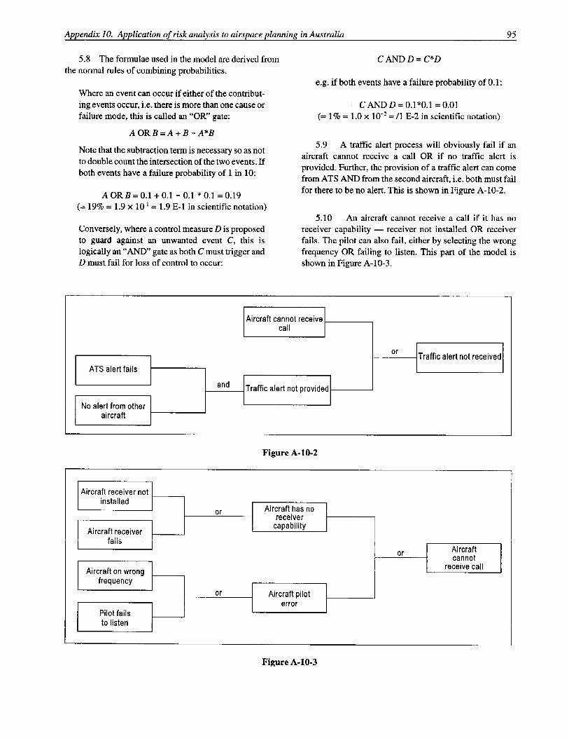

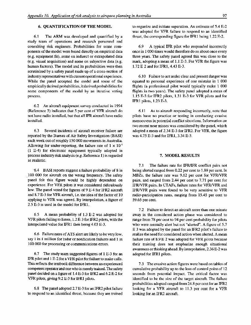


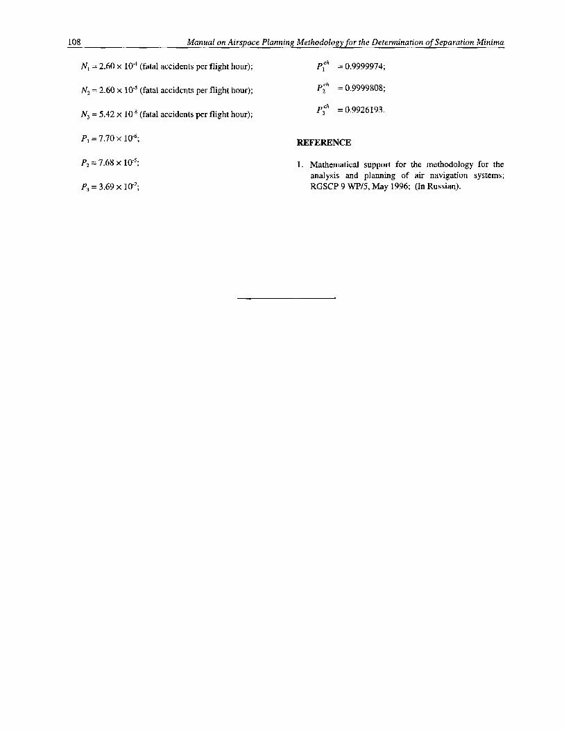

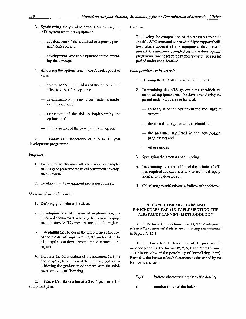
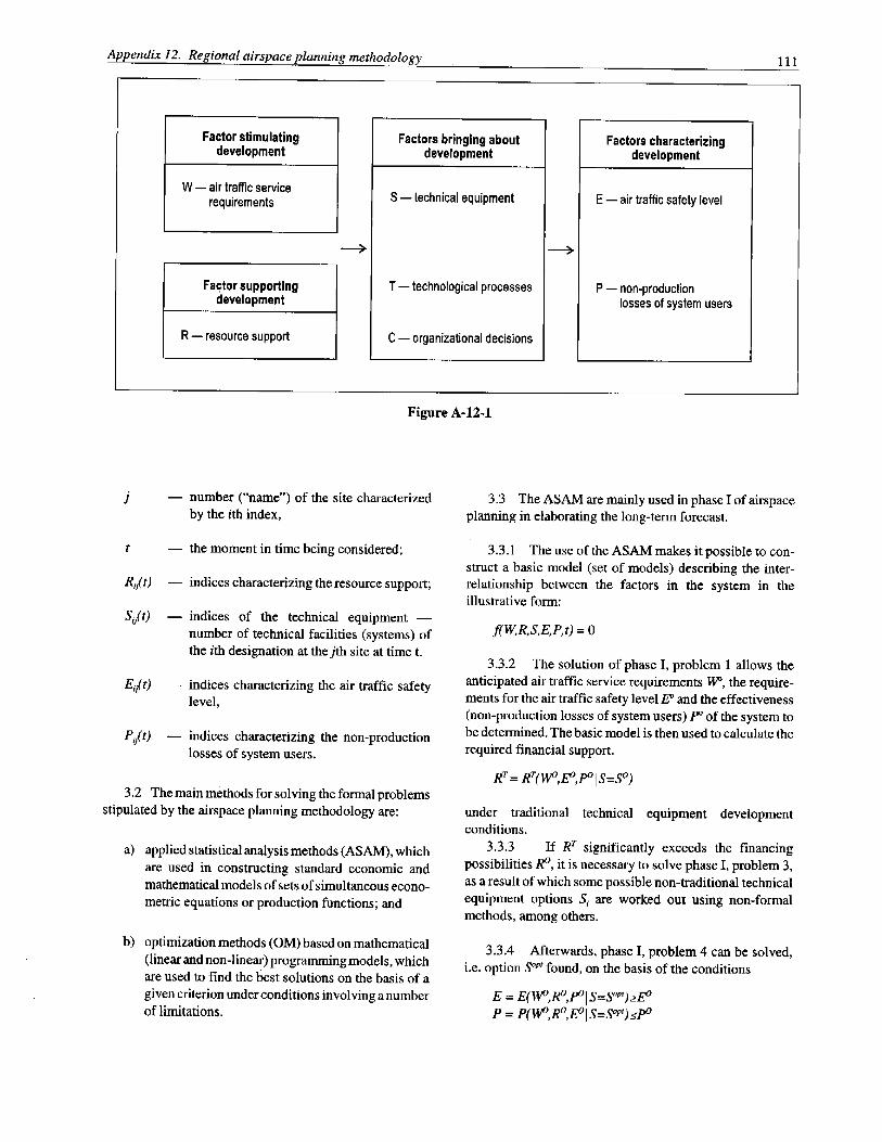

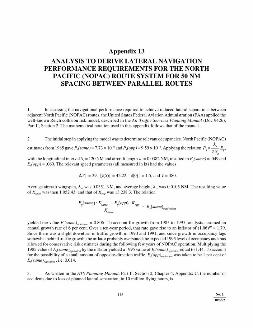
Appendix 13ANALYSIS TO DERIVE LATERAL NAVIGATION
PERFORMANCE REQUIREMENTS FOR THE NORTHPACIFIC (NOPAC) ROUTE SYSTEM FOR 50 NM
SPACING BETWEEN PARALLEL ROUTES
1. In assessing the navigational performance required to achieve reduced lateral separations betweenadjacent North Pacific (NOPAC) routes, the United States Federal Aviation Administration (FAA) applied thewell-known Reich collision risk model, described in the Air Traffic Services Planning Manual (Doc 9426),Part II, Section 2. The mathematical notation used in this appendix follows that of the manual.
2. The initial step in applying the model was to determine relevant occupancies. North Pacific (NOPAC)
estimates from 1985 gave Px(same) = 7.73 × 10�6 and Px(opp) = 9.59 × 10�6. Applying the relation ,
with the longitudinal interval Sx = 120 NM and aircraft length �x = 0.0382 NM, resulted in Ey(same) = .049 andEy(opp) = .060. The relevant speed parameters (all measured in kt) had the values
= 29, = 42.22, = 1.5, and V = 480.
Average aircraft wingspan, �y, was 0.0351 NM, and average height, �z, was 0.0105 NM. The resulting valueof Ksame was then 1 052.43, and that of Kopp was 13 238.3. The relation
yielded the value Ey(same)equivalent = 0.806. To account for growth from 1985 to 1995, analysts assumed anannual growth rate of 6 per cent. Over a ten-year period, that rate gave rise to an inflator of (1.06)10 = 1.79.Since there was a slight downturn in traffic growth in 1990 and 1991, and since growth in occupancy lagssomewhat behind traffic growth, the inflator probably overstated the expected 1995 level of occupancy and thusallowed for conservative risk estimates during the following few years of NOPAC operation. Multiplying the1985 value of Ey(same)equivalent by the inflator yielded a 1995 value of Ey(same)equivalent equal to 1.44. To accountfor the possibility of a small amount of opposite-direction traffic, Ey(opp)equivalent was taken to be 1 per cent ofEy(same)equivalent , i.e. 0.014.
3. As written in the ATS Planning Manual, Part II, Section 2, Chapter 4, Appendix C, the number ofaccidents due to loss of planned lateral separation, in 10 million flying hours, is
113 No. 1
30/8/02

114 Manual on Airspace Planning Methodology for the Determination of Separation Minima
No. 1
30/8/02
.
FAA analysts used the 1995 values of Ey(same)equivalent and Ey(opp)equivalent to respectively represent Ey(same) andEy(opp) in this basic equation. They took the value of Pz(0) to be 0.38, and the values of all other parameterson the right side of the equation, except Py(S), were those given above. Taking a maximum tolerable value of0.2 for Nay, they then solved to obtain a maximum tolerable lateral overlap probability Py(S) = 9.66 × 10�8.
4. For many years aircraft lateral errors have been modelled as double double exponential (DDE) randomvariables. The probability density function of a DDE random variable has the form
in which the parameters �, �1 and �2 satisfy the conditions 0 < � < 1, and 0 < �1 < �2. When two parallel routesare separated by a distance S, the probability that aeroplanes assigned to different routes have laterallyoverlapping positions is
The sum enclosed in rectangular brackets on the right side of this equation consists of three terms of which the
second, , contributes very little. The first term, , dominates the sum
when �1 is more than (approximately) S/15. However, in September 1992, the Review of the General Conceptof Separation Panel (RGCSP) Working Group A determined that required navigation performance (RNP) foroceanic flight should be set small enough to keep �1 well below that value (preferably no more than S/18) andthus reduce the influence of the first term to a negligible amount. The result of this approach, therefore, is torender the third term dominant. That is, when RNP is less than S/6, the three-term sum in brackets consists
almost entirely of the term . Furthermore, since is normally quite
small, whenever �1 is small, the third term can be approximated quite accurately by the simpler expression

Appendix 13. Analysis to derive lateral navigation performance requirementsfor the North Pacific (NOPAC) route system for 50 NM spacing between parallel routes 115
No. 1
30/8/02
. Under those circumstances, Py(S) � . As a function of , has one local maximum,
which occurs at �2 = S. Its value there is . By choosing �2 = S, � can conservatively be taken to have the
value = .000187.
5. As was mentioned above, aircraft using parallel routes separated by 50 NM should meet an RNP of50/6 NM. Since the RGCSP preferred integer values of RNP, FAA analysts assumed that the RNP of such a
route system would be the next smallest integer, i.e. 8 NM. The corresponding value of �1 is
Thus if the lateral errors of the fleet using the route system are characterized by a DDE density, its parametersmust be no worse than � = 0.000187, �1 = 2.6705, and �2 = 50.
6. It is possible to express the navigational performance required for operation in the planned routesystem in somewhat simpler terms. The value of �1 corresponds to a standard deviation of typical lateral errorsof , or 3.78 NM. The gross error performance can also be described more simply. As is done in NorthAtlantic minimum navigation performance specification (MNPS) airspace, aircraft could be constrained tospend all but a certain proportion, �, of their flying time within one-half separation standard (i.e. within S/2)of their route centre lines, and they could be constrained to spend all but another proportion of their flying time,�, more than some established distance (e.g. 10 NM) away from either adjacent route’s centre line. Byintegrating the DDE density function specified above, between appropriate limits (i.e. by evaluating the DDEdistribution function at appropriate points), FAA analysts found the values of � and � to be � = 1.994 � 10�4 �2.0 � 10�4 and � = 2.802 � 10�5 � 2.8 � 10�5. Table A-13-1 summarizes the two (equivalent) means of describingthe navigational performance required of the NOPAC fleet in order for Nay, the number of accidents expectedin 10 million NOPAC flight hours, to remain less than the maximum tolerable value of 0.2.
Table A-13-1. Two (equivalent) means of describingthe navigational performance required of the NOPAC fleet
DDE distribution � = 0.000187 �1 = 2.67 NM �2 = 50 NM
Navigation constraint RNP = 8 NM � = 2.0 x 10�4 � = 2.8 x 10�5
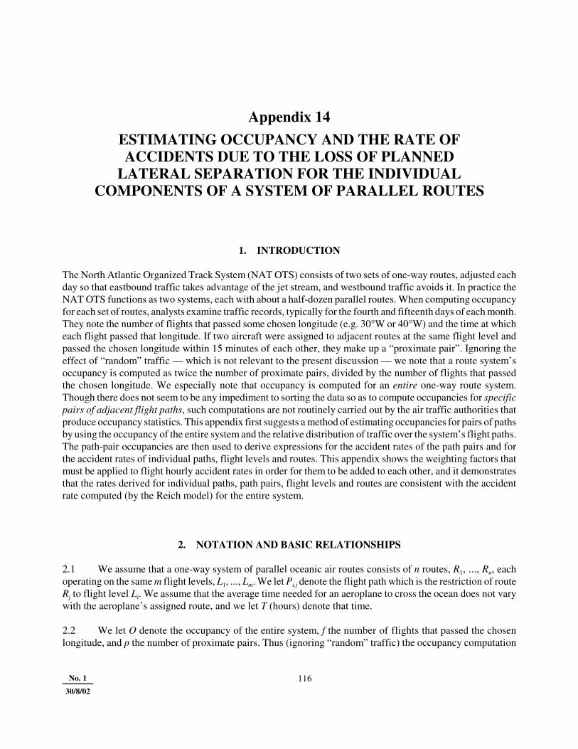
Appendix 14ESTIMATING OCCUPANCY AND THE RATE OFACCIDENTS DUE TO THE LOSS OF PLANNED
LATERAL SEPARATION FOR THE INDIVIDUALCOMPONENTS OF A SYSTEM OF PARALLEL ROUTES
1. INTRODUCTION
The North Atlantic Organized Track System (NAT OTS) consists of two sets of one-way routes, adjusted eachday so that eastbound traffic takes advantage of the jet stream, and westbound traffic avoids it. In practice theNAT OTS functions as two systems, each with about a half-dozen parallel routes. When computing occupancyfor each set of routes, analysts examine traffic records, typically for the fourth and fifteenth days of each month.They note the number of flights that passed some chosen longitude (e.g. 30°W or 40°W) and the time at whicheach flight passed that longitude. If two aircraft were assigned to adjacent routes at the same flight level andpassed the chosen longitude within 15 minutes of each other, they make up a “proximate pair”. Ignoring theeffect of “random” traffic — which is not relevant to the present discussion — we note that a route system’soccupancy is computed as twice the number of proximate pairs, divided by the number of flights that passedthe chosen longitude. We especially note that occupancy is computed for an entire one-way route system.Though there does not seem to be any impediment to sorting the data so as to compute occupancies for specificpairs of adjacent flight paths, such computations are not routinely carried out by the air traffic authorities thatproduce occupancy statistics. This appendix first suggests a method of estimating occupancies for pairs of pathsby using the occupancy of the entire system and the relative distribution of traffic over the system’s flight paths.The path-pair occupancies are then used to derive expressions for the accident rates of the path pairs and forthe accident rates of individual paths, flight levels and routes. This appendix shows the weighting factors thatmust be applied to flight hourly accident rates in order for them to be added to each other, and it demonstratesthat the rates derived for individual paths, path pairs, flight levels and routes are consistent with the accidentrate computed (by the Reich model) for the entire system.
2. NOTATION AND BASIC RELATIONSHIPS
2.1 We assume that a one-way system of parallel oceanic air routes consists of n routes, R1, ..., Rn, eachoperating on the same m flight levels, L1, ..., Lm. We let Pi,j denote the flight path which is the restriction of routeRj to flight level Li. We assume that the average time needed for an aeroplane to cross the ocean does not varywith the aeroplane’s assigned route, and we let T (hours) denote that time.
2.2 We let O denote the occupancy of the entire system, f the number of flights that passed the chosenlongitude, and p the number of proximate pairs. Thus (ignoring “random” traffic) the occupancy computation
No. 1 11630/8/02

Appendix 14. Estimating occupancy and the rate of accidents due to the loss of plannedlateral separation for the individual components of a system of parallel routes 117
No. 1
30/8/02
applies the equation . Reports of occupancy computations normally indicate the observed values of f
and p, as well as the value of O derived from them.
2.3 We parenthetically note that Appendix 13 derives another method of computing occupancy, viz. themethod given in the Air Traffic Services Planning Manual (Doc 9426). Doc 9426 defines occupancy to meantwice the ratio of route-system proximity time to route-system flight time, but it is easy to see that this definitionis essentially equivalent to the definition in 1.1 and 2.2. By virtue of the “snapshot” principle (the uniformityassumption that underlies much of collision risk theory for systems of parallel routes) the number of observedpairs, p, is the same at any observation point along the route system (though the specific pairs observed at onepoint are not necessarily the ones observed at another point). Since T denotes the number of hours needed totraverse the ocean on any of the system’s routes, we see that there are pT hours of proximity time and fT hoursof flight time during the observation period. Thus twice the ratio of proximity time to flight time is simply
, or (QED).
2.4 Given a pair of adjacent paths at the same altitude, Pi,j and Pi,j+1 (1 � i � m, 1 � j � n�1), we let Oi,j
denote their occupancy. We do not know the number of flights counted on each path, but it can nonetheless begiven a name. We let fi,j be the number of flights that passed the chosen longitude while assigned to path Pi,j
(1 � i � m, 1 � j � n), and we let pi,j be the number of proximate pairs that consisted of one aeroplane from Pi,j
and one aeroplane from Pi,j+1 (1 � i � m, 1 � j � n�1). Though we do not know the numerical values of the fi,j
and pi,j, we do know that every flight is on exactly one path so that , and every proximate pair
belongs to exactly one pair of adjacent paths so that .
3. OCCUPANCY OF A SPECIFICPAIR OF PATHS
3.1 Restricting our attention to a particular pair of adjacent paths at the same flight level, Pk,l and Pk,l+1, wecompute the pair’s occupancy as twice the number of proximate (aircraft) pairs having one member from eachpath, divided by the total number of flights on the two paths. That is:
Ok,l ,
provided that fk,l and fk,l+1 are not both 0. If they are both 0, we take Ok,l to be 0, since it would not make senseto imagine non-zero occupancy for a pair of paths that do not have any traffic.
3.2 Lacking empirical knowledge of the numbers pi,j, we can nevertheless make a reasonable assumptionas to their distribution. We expect pk,l , the number of proximate aircraft pairs associated with paths Pk,l and Pk,l+1,to be proportional to fk,l � fk,l+1 , the product of the traffic levels realized on those two paths. In particular, we

118 Manual on Airspace Planning Methodology for the Determination of Separation Minima
No. 1
30/8/02
assume that pk,l If fk,l = 0 or fk,l+1 = 0, then pk,l must be 0, and in that case Ok,l must also
be 0, which agrees with our intuitive understanding that a path pair exhibits zero occupancy when either of itsmembers does not have any traffic. In the rest of this appendix we assume that fk,l and fk,l+1 are both non-zero.
3.3 The assumption of proportionality in the last paragraph is an approximation whose accuracy needs tobe determined by empirical studies. In particular we note that in any data collection the numbers of proximatepairs, pi,j , would be integers, yet we have no guarantee that the formula for pk,l will yield an integer. However,the formula does satisfy the conservation criterion stated as the last equation of the previous section:
3.4 In order to develop an expression for Ok,l in terms of O, we adopt a simplifying notation. For each path
Pi,j , let ri,j denote the quotient . Each ri,j is then the fraction of the route system’s traffic that travelled on
path Pi,j , so
Recalling the expression for Ok,l in 3.1, we apply this new notation to the factor , rewriting it as
. We also take advantage of this notation to rewrite the number of proximate pairs
belonging to each path pair:
pk,l = = = .
At least one pair of adjacent flight paths must have positive traffic loads on both of its paths (otherwise thereis no occupancy to compute) so in the denominator at least one term, ri,j � ri,j+1, is positive, and we can be surethat the denominator is non-zero.
3.5 We can now substitute the expressions derived in the last three paragraphs into the expression for Ok,l
that was given in 3.1. We find that
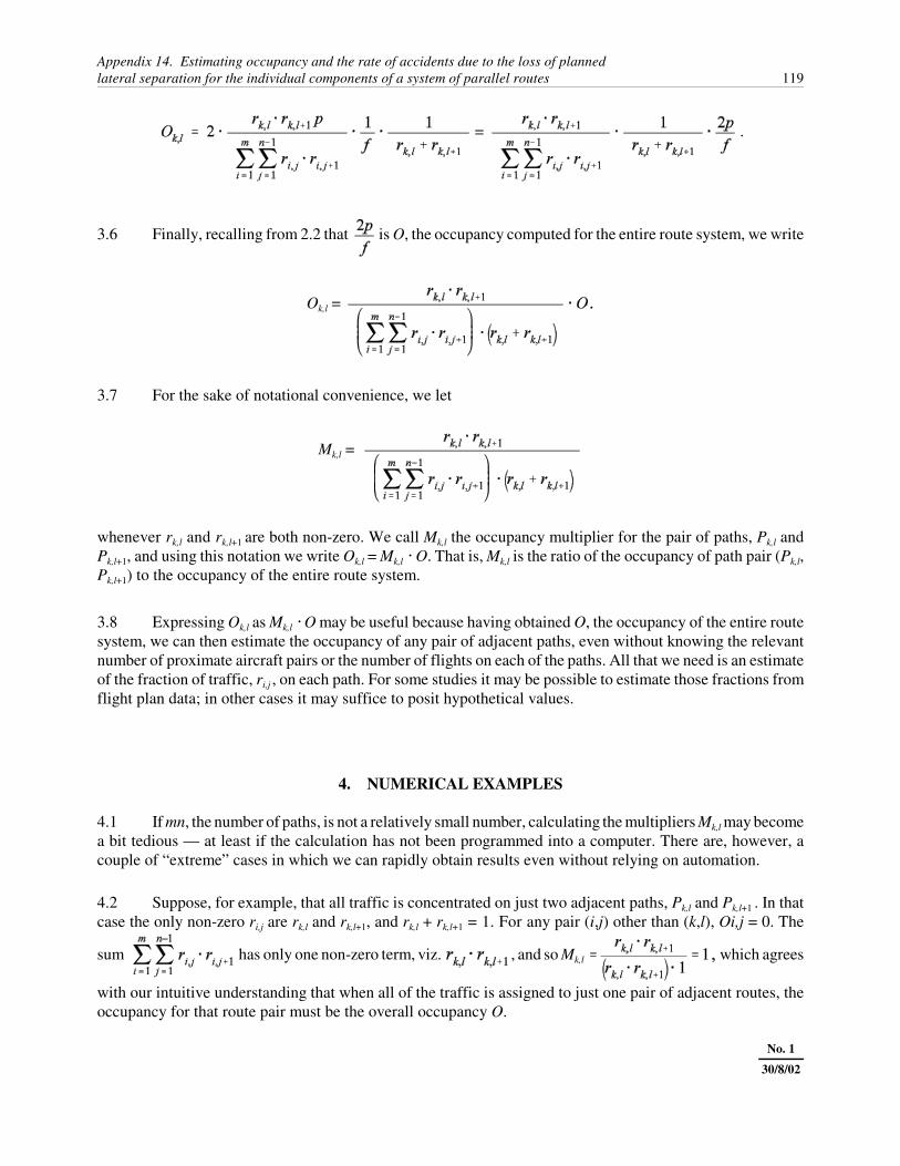
Appendix 14. Estimating occupancy and the rate of accidents due to the loss of plannedlateral separation for the individual components of a system of parallel routes 119
No. 1
30/8/02
= .
3.6 Finally, recalling from 2.2 that is O, the occupancy computed for the entire route system, we write
Ok,l =
3.7 For the sake of notational convenience, we let
Mk,l =
whenever rk,l and rk,l+1 are both non-zero. We call Mk,l the occupancy multiplier for the pair of paths, Pk,l andPk,l+1, and using this notation we write Ok,l = Mk,l � O. That is, Mk,l is the ratio of the occupancy of path pair (Pk,l,Pk,l+1) to the occupancy of the entire route system.
3.8 Expressing Ok,l as Mk,l � O may be useful because having obtained O, the occupancy of the entire routesystem, we can then estimate the occupancy of any pair of adjacent paths, even without knowing the relevantnumber of proximate aircraft pairs or the number of flights on each of the paths. All that we need is an estimateof the fraction of traffic, ri,j , on each path. For some studies it may be possible to estimate those fractions fromflight plan data; in other cases it may suffice to posit hypothetical values.
4. NUMERICAL EXAMPLES
4.1 If mn, the number of paths, is not a relatively small number, calculating the multipliers Mk,l may becomea bit tedious — at least if the calculation has not been programmed into a computer. There are, however, acouple of “extreme” cases in which we can rapidly obtain results even without relying on automation.
4.2 Suppose, for example, that all traffic is concentrated on just two adjacent paths, Pk,l and Pk,l+1 . In thatcase the only non-zero ri,j are rk,l and rk,l+1, and rk,l + rk,l+1 = 1. For any pair (i,j) other than (k,l), Oi,j = 0. The
sum has only one non-zero term, viz. , and so Mk,l which agrees
with our intuitive understanding that when all of the traffic is assigned to just one pair of adjacent routes, theoccupancy for that route pair must be the overall occupancy O.

120 Manual on Airspace Planning Methodology for the Determination of Separation Minima
No. 1
30/8/02
4.3 Table A-14-1 shows a spreadsheet that calculates the multipliers Mk,l for a route system having fourroutes at each of three flight levels. With two exceptions, the numbers inserted into column “r(i,j)”, whichshows the fraction of traffic on each path, are all zero. The two exceptions are for routes R2 and R3 on flightlevel L2. Path P2,2 has 30 per cent of the system’s traffic, while P2,3 carries the remaining 70 per cent. Thespreadsheet calculates an occupancy multiplier of 1 for that pair of paths and shows the code “NA” (“notapplicable”) for all other multipliers.
4.4 A much more interesting case occurs when we consider the traffic to be uniformly distributed over all
mn flight paths. In that case, each ri,j , and so
Mk,l
for every pair of paths, Pk,l and Pk,l+1, i.e. for every pair of adjacent paths at the same flight level. We note thatthis formula for Mk,l is independent of m, the number of flight levels in the system, and we also observe that asn increases, Mk,l approaches 1/2 from above.
4.5 Table A-14-2 shows a spreadsheet similar to that of Table A-14-1, but the numbers in column “r(i,j)”are all 1/12 = .0833, which is the fraction of traffic borne by each flight path when the traffic is uniformlydistributed over all 12 paths. Since n, the number of routes, is 4, the formula derived in the last paragraph tells
us that the multipliers must all be , and indeed Table A-14-2 shows that the spreadsheet calculates
all of the occupancy multipliers to be 0.6667.
4.6 Empirical studies may eventually show that for certain traffic distributions the assumption ofproportionality (in 3.2) does not accurately describe the distribution of proximate pairs. However, theassumption must be accurate for the case in which the traffic is uniformly distributed. When all flight pathscarry the same load, the assumption infers that every pair of adjacent paths produces the same number ofproximate aircraft pairs. That is not surprising. As long as the theory treats the number of proximate pairsproduced by a pair of paths as a function solely of the traffic loads on those paths, it follows that whenever thepaths all carry the same load, every pair of paths must produce the same number of proximate aircraft pairs,regardless of the specific form of the function. That is, if g denotes the function, then pi,j = for
1 � i � m, 1 � j � n�1. If the traffic is uniformly distributed, then every fi,j and fi,j+1 has the same value, viz. ,
and so every pi,j . Therefore, p so
, which clearly does not depend on either i or j.
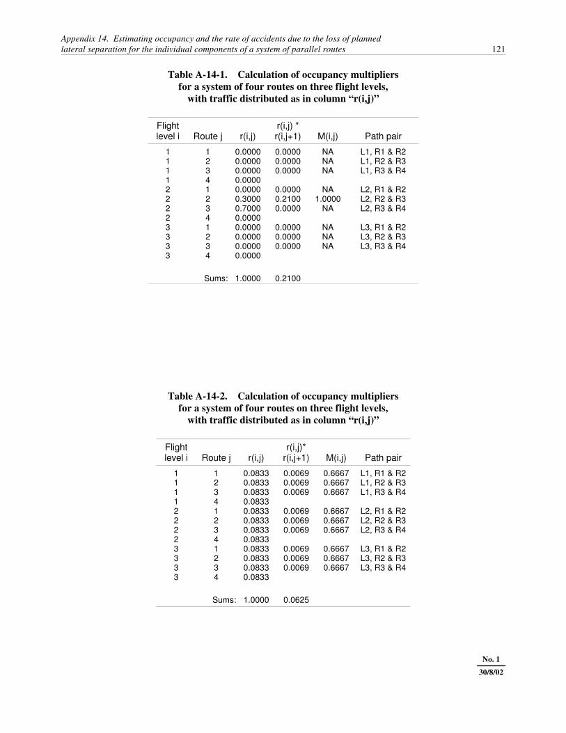
Appendix 14. Estimating occupancy and the rate of accidents due to the loss of plannedlateral separation for the individual components of a system of parallel routes 121
No. 1
30/8/02
Table A-14-1. Calculation of occupancy multipliersfor a system of four routes on three flight levels,
with traffic distributed as in column “r(i,j)”
Flightlevel i Route j r(i,j)
r(i,j) *r(i,j+1) M(i,j) Path pair
1 1 0.0000 0.0000 NA L1, R1 & R21 2 0.0000 0.0000 NA L1, R2 & R31 3 0.0000 0.0000 NA L1, R3 & R41 4 0.00002 1 0.0000 0.0000 NA L2, R1 & R22 2 0.3000 0.2100 1.0000 L2, R2 & R32 3 0.7000 0.0000 NA L2, R3 & R42 4 0.00003 1 0.0000 0.0000 NA L3, R1 & R23 2 0.0000 0.0000 NA L3, R2 & R33 3 0.0000 0.0000 NA L3, R3 & R43 4 0.0000
Sums: 1.0000 0.2100
Table A-14-2. Calculation of occupancy multipliersfor a system of four routes on three flight levels,
with traffic distributed as in column “r(i,j)”
Flightlevel i Route j r(i,j)
r(i,j)*r(i,j+1) M(i,j) Path pair
1 1 0.0833 0.0069 0.6667 L1, R1 & R21 2 0.0833 0.0069 0.6667 L1, R2 & R31 3 0.0833 0.0069 0.6667 L1, R3 & R41 4 0.08332 1 0.0833 0.0069 0.6667 L2, R1 & R22 2 0.0833 0.0069 0.6667 L2, R2 & R32 3 0.0833 0.0069 0.6667 L2, R3 & R42 4 0.08333 1 0.0833 0.0069 0.6667 L3, R1 & R23 2 0.0833 0.0069 0.6667 L3, R2 & R33 3 0.0833 0.0069 0.6667 L3, R3 & R43 4 0.0833
Sums: 1.0000 0.0625

122 Manual on Airspace Planning Methodology for the Determination of Separation Minima
No. 1
30/8/02
4.7 Table A-14-3 shows the same sort of spreadsheet shown in Tables A-14-1 and A-14-2, but with atypical traffic distribution. Flight level L1 carries 1/4 of the traffic, L2 has 5/12 of it, and L3 has the remaining1/3. On each flight level, route R1 has 1/12 of the traffic, R2 has 1/3 of it, R3 has 5/12 of it, and R4 has theremaining 1/6. The occupancy multipliers calculated by the spreadsheet range from a minimum value of 0.2033,for path pair (P1,1 , P1,2), to a maximum of 0.9412 for path pair (P2,2 , P2,3).
4.8 In the examples given so far, Mk,l has been less than or equal to 1, but that does not hold true in general.
Indeed, we see from the definition (in 3.7) that Mk,l � 1 if and only if �
Table A-14-4 shows a traffic distribution derived from that of Table A-14-3 by shifting traffic from one pathto another. In particular, the loads on paths P1,2 , P1,4 , P3,1 , and P3,3 were respectively shifted onto paths P1,1 ,P1,3 , P3,2 , and P3,4 , so that all six pairs of adjacent paths on flight levels L1 and L3 have zero occupancy. As canbe seen in the column headed “r(i,j)*r(i,j+1)”, the three products are all zero, as are the three products
. The sum is less than and , and so M2,2 = 1.8824 and M2,3 =
1.2101 are both greater than 1.
5. ACCIDENT RATES FOR PAIRS OFADJACENT FLIGHT PATHS
5.1 Let ak,l denote the expected rate of accidents for the pair of paths Pk,l and Pk,l+1. In the Reich model forthe risk of collision due to the loss of planned lateral separation, we write ak,l as a product of 5 factors: 1) theprobability that two aeroplanes which are assigned to adjacent paths actually have laterally overlappingpositions; 2) the probability that two aeroplanes assigned to the same flight level have vertically overlappingpositions; 3) the probability that two proximate aeroplanes (proximate in the sense of 1.1) have longitudinallyoverlapping positions; 4) the sum of the reciprocals of the times needed for aircraft to pass each other in eachof the three physical dimensions; and 5) the occupancy, Ok,l, of the pair Pk,l and Pk,l+1. The accident rate ak,l isexpressed in units of accidents per flight hour.
5.2 In the present discussion we are not concerned with changes in any of the first four factors mentionedin 5.1 and can assume that they are invariant over all pairs of paths. Therefore, we can simplify the notationin the present section by expressing the product of the first four factors as a constant C. That is, for every pairof paths Pk,l and Pk,l+1, ak,l = C � Ok,l. Using the results of section 3, we rewrite this equation as
.
Since C�O is the accident rate of the entire system (in accidents per flight hour), Mk,l is also the ratio of theaccident rate of path pair (Pk,l , Pk,l+1) to that of the entire system. We also find it useful to express the equationfor ak,l in one more form, i.e. as

Appendix 14. Estimating occupancy and the rate of accidents due to the loss of plannedlateral separation for the individual components of a system of parallel routes 123
No. 1
30/8/02
Table A-14-3. Calculation of occupancy multipliersfor a system of four routes on three flight levels,
with traffic distributed as in column “r(i,j)”
Flightlevel i Route j r(i,j)
r(i,j)*r(i,j+1) M(i,j) Path pair
1 1 0.0208 0.0017 0.2033 L1, R1 & R21 2 0.0833 0.0087 0.5647 L1, R2 & R31 3 0.1042 0.0043 0.3630 L1, R3 & R41 4 0.04172 1 0.0347 0.0048 0.3388 L2, R1 & R22 2 0.1389 0.0241 0.9412 L2, R2 & R32 3 0.1736 0.0121 0.6050 L2, R3 & R42 4 0.06943 1 0.0278 0.0031 0.2711 L3, R1 & R23 2 0.1111 0.0154 0.7529 L3, R2 & R33 3 0.1389 0.0077 0.4840 L3, R3 & R43 4 0.0556
Sums: 1.0000 0.0820
Table A-14-4. Calculation of occupancy multipliersfor a system of four routes on three flight levels,
with traffic distributed as in column “r(i,j)”
Flightlevel i Route j r(i,j)
r(i,j)*r(i,j+1) M(i,j) Path pair
1 1 0.1042 0.0000 NA L1, R1 & R21 2 0.0000 0.0000 NA L1, R2 & R31 3 0.1458 0.0000 NA L1, R3 & R41 4 0.00002 1 0.0347 0.0048 0.6776 L2, R1 & R22 2 0.1389 0.0241 1.8824 L2, R2 & R32 3 0.1736 0.0121 1.2101 L2, R3 & R42 4 0.06943 1 0.0000 0.0000 NA L3, R1 & R23 2 0.1389 0.0000 NA L3, R2 & R33 3 0.0000 0.0000 NA L3, R3 & R43 4 0.1944
Sums: 1.0000 0.0410

124 Manual on Airspace Planning Methodology for the Determination of Separation Minima
No. 1
30/8/02
.
5.3 Let T denote the time needed for a typical aeroplane to cross the ocean on the route system. During the24-hour period used to determine occupancy, the fk,l aeroplanes on path Pk,l contributed T � fk,l flight hours. Thus
path Pk,l experienced a traffic load of flight hours per hour. Likewise, path Pk,l+1 experienced a traffic load
of flight hours per hour, and so the two paths experienced a (combined) traffic load of
. We can therefore express the accident rate for the pair of paths, Pk,l and Pk,l+1,
as
.
5.4 When accident rates are expressed in units of accidents per hour, we can add the rates for any two pathpairs in order to obtain the total accident rate (still in accidents per hour) for those two pairs. Thus, for example,we find the total accident rate for the path pairs (P1,2 , P1,3) and (P3,3 , P3,4) to be
.
More generally, we obtain the total accident rate for all of the pairs in a set of path pairs by simply adding therates (in accidents per hour) for the pairs in that set.
5.5 We can then convert the total rate from units of accidents per hour to units of accidents per flight hour.In the example in the last paragraph, path pairs (P1,2 , P1,3) and (P3,3 , P3,4) experienced
flight hours during the 24-hour period used to determine occupancy, so their traffic load was at the rate of
. Expressed in traditional units, the two path pairs had a combined
accident rate of
,

Appendix 14. Estimating occupancy and the rate of accidents due to the loss of plannedlateral separation for the individual components of a system of parallel routes 125
No. 1
30/8/02
and when the numerator and denominator are divided by f, we re-express this rate as
.
5.6 Similarly, the accident rate for all of flight level Lk is
,
and the accident rate for the route pair (Rl,Rl+1) is
.
Note that in the formula for Lk, the denominator shows each path’s flow counted once, even though all but theoutermost paths belong to two path pairs.
5.7 Finally, we write the accident rate of the entire system, in accidents per hour, as
.
During the 24-hour period used to determine occupancy, the system experienced Tf flight hours, giving it a
traffic rate of . Expressed in traditional units, the entire route system had an accident rate of
.

126 Manual on Airspace Planning Methodology for the Determination of Separation Minima
No. 1
30/8/02
However, we also know from 5.2 that each . Substituting this
expression into the sum, we find the accident rate of the entire route system to be
which is exactly the result that we expected from the Reich model. Thus we find that the formulae derivedabove for the accident rates of path pairs and collections of path pairs are consistent with the accepted model.
6. ACCIDENT RATES FOR INDIVIDUAL FLIGHT PATHS
6.1 Paths Pk,1 and Pk,n are the outer paths on flight level Lk, so each of them has only one adjacent path onthat flight level. The aeroplanes on Pk,1 are exposed to risk from those on Pk,2 , while the aeroplanes on Pk,n areexposed to risk from those on Pk,n–1 . If 2 � l � n�1, the aeroplanes on path Pk,l are exposed to the risk ofcollision with aeroplanes on two adjacent paths, Pk,l�1 and Pk,l+1 .
6.2 The rate of accidents for the path pair (Pk,1 , Pk,2) is . As was shown in 5.3, we can re-
express this rate as . Every collision due to the loss of planned lateral separation
is counted as two accidents, each involving an aeroplane assigned to one of the relevant paths. Therefore, path
Pk,1 has an accident rate of . Path Pk,1 experiences flight hours in
24 hours, or , so its accident rate, expressed in traditional units, is
.
Dividing the numerator and denominator by f, we re-write Pk,1’s accident rate as
.
Applying entirely analogous reasoning, we find that the hourly rate for path Pk,n is
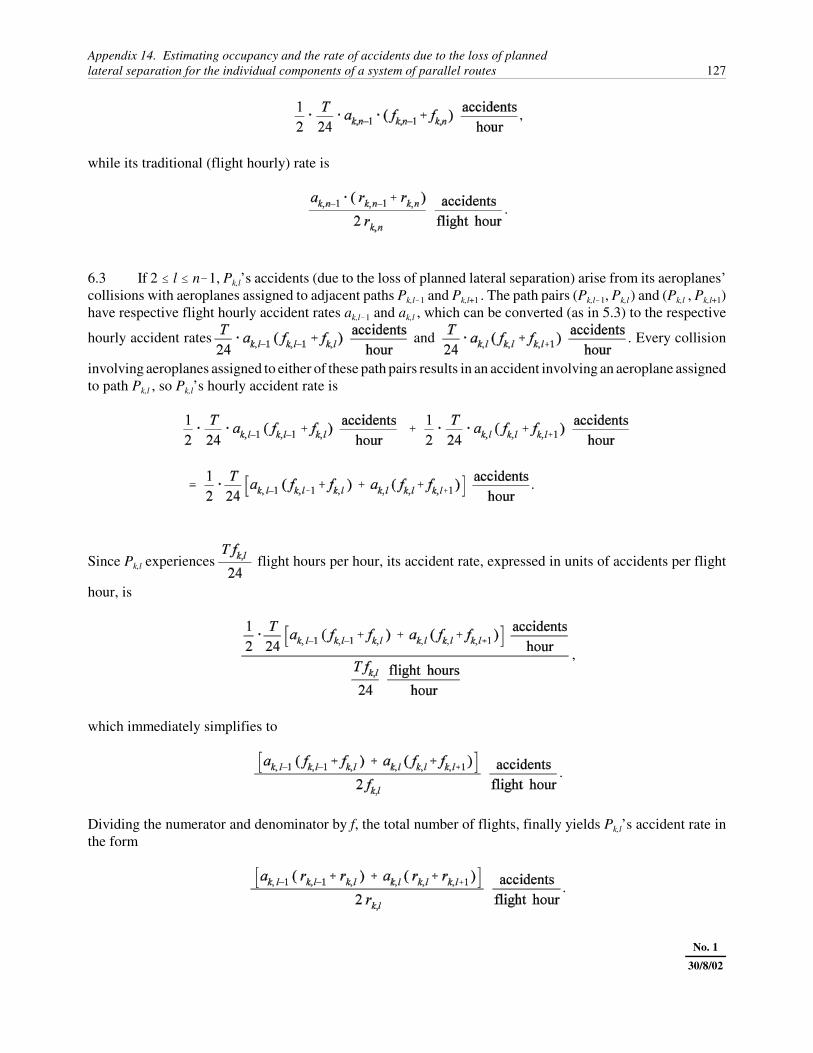
Appendix 14. Estimating occupancy and the rate of accidents due to the loss of plannedlateral separation for the individual components of a system of parallel routes 127
No. 1
30/8/02
,
while its traditional (flight hourly) rate is
.
6.3 If 2 � l � n�1, Pk,l’s accidents (due to the loss of planned lateral separation) arise from its aeroplanes’collisions with aeroplanes assigned to adjacent paths Pk,l�1 and Pk,l+1 . The path pairs (Pk,l�1, Pk,l ) and (Pk,l , Pk,l+1)have respective flight hourly accident rates ak,l�1 and ak,l , which can be converted (as in 5.3) to the respective
hourly accident rates and . Every collision
involving aeroplanes assigned to either of these path pairs results in an accident involving an aeroplane assignedto path Pk,l , so Pk,l’s hourly accident rate is
.
Since Pk,l experiences flight hours per hour, its accident rate, expressed in units of accidents per flight
hour, is
,
which immediately simplifies to
.
Dividing the numerator and denominator by f, the total number of flights, finally yields Pk,l’s accident rate inthe form
.
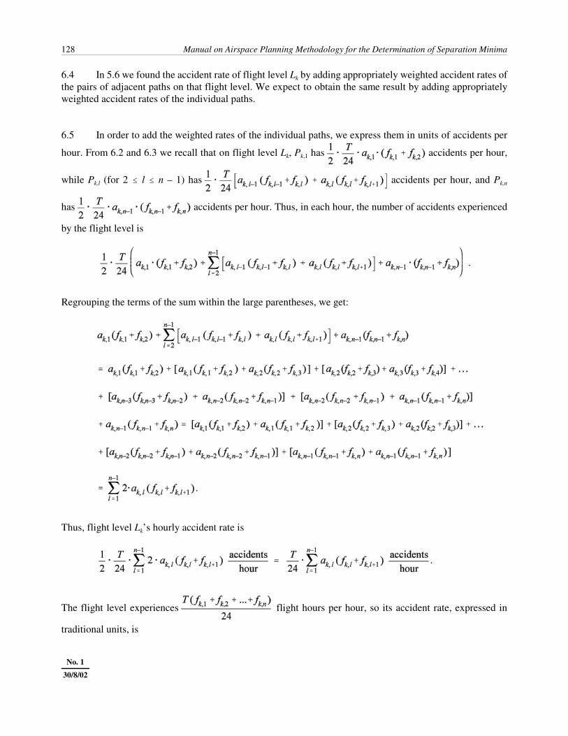
128 Manual on Airspace Planning Methodology for the Determination of Separation Minima
No. 1
30/8/02
6.4 In 5.6 we found the accident rate of flight level Lk by adding appropriately weighted accident rates ofthe pairs of adjacent paths on that flight level. We expect to obtain the same result by adding appropriatelyweighted accident rates of the individual paths.
6.5 In order to add the weighted rates of the individual paths, we express them in units of accidents per
hour. From 6.2 and 6.3 we recall that on flight level Lk, Pk,1 has accidents per hour,
while Pk,l (for 2 � l � n – 1) has accidents per hour, and Pk,n
has accidents per hour. Thus, in each hour, the number of accidents experienced
by the flight level is
.
Regrouping the terms of the sum within the large parentheses, we get:
.
Thus, flight level Lk’s hourly accident rate is
.
The flight level experiences flight hours per hour, so its accident rate, expressed in
traditional units, is

Appendix 14. Estimating occupancy and the rate of accidents due to the loss of plannedlateral separation for the individual components of a system of parallel routes 129
No. 1
30/8/02
,
which agrees with the result stated at the beginning of 5.6.
6.6 We use a similar technique to find the accident rate for any of the n routes in the system. Route R1
consists of paths Pi,1 for i = 1, 2, ..., m, and in 6.2 we noted that Pi,1 experiences accidents
per hour. Adding the hourly rates we find that R1 has accidents per hour. Since it
experiences flight hours of traffic in 24 hours, its accident rate in traditional units is
.
Analogous reasoning shows that Rn’s accident rate is .
6.7 If 2 � j � n–1, then (as noted in 6.3) each path Pi,j has
accidents per hour, so that route Rj has . Since Rj

130 Manual on Airspace Planning Methodology for the Determination of Separation Minima
No. 1
30/8/02
experiences flight hours per hour, its accident rate, expressed in traditional units, is
,
which immediately simplifies to
.
Dividing the numerator and denominator by f, we re-express the accident rate of route Rj in terms of trafficratios as
.
6.8 In 6.5 we showed that flight level Li experiences accidents per hour. Adding the
hourly rates for all the flight levels, we see that the entire route system experiences
. This is the same hourly rate cited at the beginning of 5.7, where the sum
was derived from the hourly accident rates of path pairs, rather than those of individual paths. Without repeatingthe argument in that paragraph, we see that the flight hourly accident rate for the entire route system, computedfrom the rates of individual paths, remains consistent with the rate computed by the Reich model.
7. OCCUPANCIES FOR PAIRS OF NON-ADJACENT ROUTES
7.1 The traditional definition of lateral occupancy applies only to adjacent routes, and so occupancycomputations generally count two aeroplanes as proximate only if they are assigned to adjacent co-altitude flightpaths. Since the risk of collision (due to the loss of planned lateral separation) between aeroplanes assigned toadjacent routes is far greater than the risk of collision between aeroplanes assigned to non-adjacent routes,traditional occupancy estimates generally account for most of the exposure to risk. However, as airspacemanagement authorities decrease route separations, it is reasonable to expect an increase in the risk of collisionbetween aeroplanes assigned to non-adjacent routes. While that risk is likely to remain much lower than the risk

Appendix 14. Estimating occupancy and the rate of accidents due to the loss of plannedlateral separation for the individual components of a system of parallel routes 131
No. 1
30/8/02
from aeroplanes assigned to adjacent routes, it may eventually constitute a significant part of the total risk.Indeed, the simplest way to determine whether it is significant is to compute both components of the risk andcompare them. The present section develops formulae that can be used to estimate the lateral occupancy of pairsof non-adjacent flight paths. Those estimates can be used to compute the rate of collisions between aeroplanesassigned to non-adjacent paths, by applying a formula similar to the one given in 5.1 and 5.2.
7.2 We begin by deriving occupancies for paths whose lateral separation is twice the minimum distance.Thus we are dealing with pairs of paths (Pi,j , Pi,j+2 ), for 1 � i � m and 1 � j � n�2. Each path Pi,j still carries fi,j
aeroplanes over a 24-hour period, so the route system carries a total of aeroplanes during that
time. We continue to let ri,j denote , the fraction of the route system’s traffic that travels on path Pi,j. On
the other hand, we need to extend some of the notation used in sections 1 through 6. We let denote the
number of proximate pairs consisting of an aeroplane assigned to Pi,j and an aeroplane assigned to Pi,j+2, and,as in sections 1 through 6, we consider a pair to be proximate if its members pass the chosen longitude (or any
other line having an analogous function) within 15 minutes of each other. We let denote the
total number of proximate pairs obtained from routes separated by twice the lateral separation minimum. Insection 2 we could rely on having an empirically derived value for p, but in the present section we do not haveany data to justify a value for its analogue, p(2), and so another method to estimate its value will need to befound. Note that we have no particular reason to expect p and p(2) to have the same value. Indeed, since thereare m fewer path pairs separated by two separation standards than by one separation standard (i.e. m(n�2) pairsrather than m(n�1) pairs) if traffic is uniformly distributed over all of the route system’s paths, we expect p(2)
to be less than p. Finally, we let O(2) denote the occupancy that we would compute if we counted only proximatepairs from co-altitude paths separated by two separation standards. Since the route system still carries a total
of f aeroplanes, we compute O(2) by a formula analogous to that used for computing O, i.e. O(2) . (In a
system having exactly three routes, only flights assigned to the outer routes can be members of proximate pairsthat are counted by p(2). Thus it might be thought that in defining O(2) for such a system, we should take the
denominator to be the number of flights on the outer routes, i.e. , rather than f, the total number of
flights in the system. Such a definition might be useful if the rate of collisions between aeroplanes assigned tonon-adjacent routes were of some interest in itself. However, the collision rate for aeroplanes assigned to non-adjacent routes is of interest only as a component of the total collision rate, and thus the denominator needs toaccount for all flights in the system.)
7.3 In section 1 we observed that occupancy statistics are not normally produced for individual pairs ofadjacent flight paths. In section 3 we overcame this difficulty by assuming that the number of proximate pairsof aircraft for a given pair of adjacent co-altitude flight paths was proportional to the product of the traffic levelson those paths. In the present section we observe that since air traffic controllers do not attempt to coordinatethe longitudinal positions of aeroplanes assigned to different paths, the assumption of proportionality is just asvalid for pairs of non-adjacent flight paths as it is for pairs of adjacent paths. Thus, if and ,
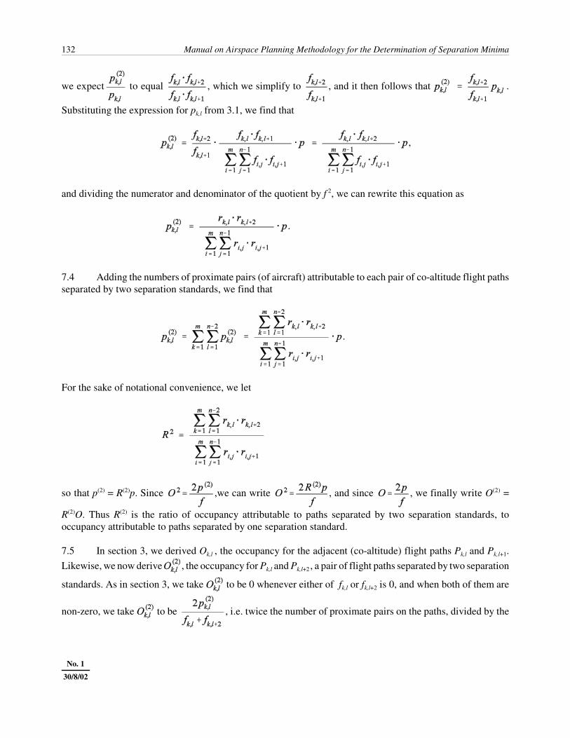
132 Manual on Airspace Planning Methodology for the Determination of Separation Minima
No. 1
30/8/02
we expect to equal , which we simplify to , and it then follows that .
Substituting the expression for pk,l from 3.1, we find that
,
and dividing the numerator and denominator of the quotient by f 2, we can rewrite this equation as
.
7.4 Adding the numbers of proximate pairs (of aircraft) attributable to each pair of co-altitude flight pathsseparated by two separation standards, we find that
.
For the sake of notational convenience, we let
so that p(2) = R(2)p. Since ,we can write , and since , we finally write O(2) =
R(2)O. Thus R(2) is the ratio of occupancy attributable to paths separated by two separation standards, tooccupancy attributable to paths separated by one separation standard.
7.5 In section 3, we derived Ok,l , the occupancy for the adjacent (co-altitude) flight paths Pk,l and Pk,l+1.Likewise, we now derive , the occupancy for Pk,l and Pk,l+2 , a pair of flight paths separated by two separation
standards. As in section 3, we take to be 0 whenever either of fk,l or fk,l+2 is 0, and when both of them are
non-zero, we take to be , i.e. twice the number of proximate pairs on the paths, divided by the
Appendix 14. Estimating occupancy and the rate of accidents due to the loss of plannedlateral separation for the individual components of a system of parallel routes 133
No. 1
30/8/02
number of flights on the paths. We then rewrite the occupancy using the formula for derived in 7.3:
.
For the sake of notational convenience, we let
= , so that .
7.6 As in section 5, where we computed accident rates for pairs of adjacent paths, accident rates for pairsof paths separated by two separation standards can likewise be computed. Only one of the constants mentionedin 5.1 changes with the increase in separation, viz. the lateral overlap probability. We recognize that change byletting C(2) denote the product of the (new) lateral overlap probability, the vertical overlap probability, thelongitudinal overlap probability for proximate aeroplanes, and the sum of the reciprocals of passing times. We
let denote the accident rate for paths Pk,l and Pk,l+2 and compute it by the Reich model formula:
. The accident rate is expressed in accidents per flight hour.
7.7 We can also express the rate of accidents between aeroplanes assigned to paths Pk,l and Pk,l+2 as anhourly rate. The paths experience a traffic load of
, or
so it follows that their hourly accident rate is
Hourly accident rates can be added to each other, and when we do so we find that the route system’s total hourlyaccident rate for accidents due to the loss of two separation standards of planned separation is

134 Manual on Airspace Planning Methodology for the Determination of Separation Minima
No. 1
30/8/02
7.8 Since the entire route system experiences , we can re-express its total accident rate
(from the loss of two separation standards of planned lateral separation) in traditional terms as
.
From 7.5 and 7.6 we know that each , and each ,
so that:
each ,
and each .
Substituting these terms into the sum above, we re-express the total accident rate, in accidents per flight hour,as
,
which is exactly the result expected from applying the Reich model.
7.9 Paragraphs 7.2 through 7.8 derive analogues of most of the significant formulae of sections 3 and 5 forthe case in which co-altitude flight paths are separated by twice the route system’s minimum lateral separation.The same reasoning can be used to derive analogous formulae for the case in which co-altitude flight paths areseparated by some other multiple of the route system’s minimum lateral separation. Without repeating thederivations, we simply list the definitions of symbols and the principal results for the case in which the flightpaths are separated by s multiples of the minimum lateral separation for any integer s between 1 and n�1:
� the number of proximate pairs consisting of an aeroplane assigned to Pi,j and an aeroplane
assigned to Pi,j+s

Appendix 14. Estimating occupancy and the rate of accidents due to the loss of plannedlateral separation for the individual components of a system of parallel routes 135
No. 1
30/8/02
p(s) � the total number of proximate pairs obtained from routes separated by a distance equal to s multiples of the lateral separation minimum
O(s) � the occupancy that would be computed by counting only proximate pairs (of aeroplanes) fromco-altitude paths separated by s separation standards
O(s) �
p(s)
R(s)
O(s) = R(s)O
C(s) � the product of the lateral overlap probability for routes separated by s multiples of the lateralseparation minimum, the vertical overlap probability, the longitudinal overlap probability forproximate aeroplanes, and the sum of reciprocals of passing times

136 Manual on Airspace Planning Methodology for the Determination of Separation Minima
No. 1
30/8/02
� the accident rate for paths Pk,l and Pk,l+s , expressed in accidents per flight hour;
.
8. CONCLUSION
8.1 The formulae derived in sections 3, 5, and 6 give analysts the tools needed to compute the accident ratesof individual components of oceanic route systems. The distribution of traffic on some of the most heavily usedroute systems is known to be markedly non-uniform, and results obtained from applying these formulae willallow decision-makers to consider not only an entire route system’s accident rate, but also the rates of the mostheavily used flight paths, routes and flight levels.
8.2 Furthermore, the formulae derived in section 7 give analysts the ability to account for risk due to theloss of planned lateral separations equal to all integer multiples of the separation minimum and thereby moreaccurately compute a route system’s total lateral risk.
— — — — — — — — — — — —

Appendix 14. Estimating occupancy and the rate of accidents due to the loss of plannedlateral separation for the individual components of a system of parallel routes 137
No. 1
30/8/02
Attachment A to Appendix 14
CONSISTENCY WITH ICAO GUIDANCE
A.1 The Air Traffic Services Planning Manual (Doc 9426) includes a discussion of the “steady state flowmodel” of occupancy (Part II, Section 2, Chapter 4, Appendix C). The present Attachment A to Appendix 14demonstrates that the steady state flow model infers the same occupancy multiplier derived in section 3 ofAppendix 14. The notation used in Doc 9426 differs from that used in Appendix 14, and the reader should notassume that symbols used in Attachment A to Appendix 14 have the same meanings they have in Appendix 14proper, unless they are specifically identified as having those meanings. In particular, subscripts in Doc 9426— and in the first part of Attachment A— reverse the order of route and flight level used in the body ofAppendix 14. Moreover, Doc 9426 uses symbols “T” and “f ” whose meanings are entirely different from thoseof the “T” and “f ” used in the body of Appendix 14.
A.2 Doc 9426 posits a system of t parallel routes operating on f flight levels. The traffic flow on the pathat route i and flight level j is mi,j aircraft per hour. Each route has length L NM, and the average speed of theaircraft on each route is V kt. The system is observed for T hours. Aircraft on adjacent paths and the same flightlevel are considered proximate when they are longitudinally within Sx NM of each other. During the T hoursin which the system is observed, Ty denotes the total time during which aircraft pairs are proximate, H denotes
the total number of flight hours, and Ey denotes the system’s occupancy. Table A-14-5 shows how the
symbols in Doc 9426 correspond to those in the body of Appendix 14.
Table A-14-5. Use of symbols
Symbol inDoc 9426
Symbol inAppendix 14 Meaning
t n Number of routes
f m Number of flight levels
mi,j Traffic flow, in aircraft per hour, on route i at flight level j
T Average time, in hours, needed to fly an oceanic route
T 24 Time, in hours, during which the system is monitored
Flight time, in hours, corresponding to a proximity interval
Ey O Occupancy

138 Manual on Airspace Planning Methodology for the Determination of Separation Minima
No. 1
30/8/02
A.3. On average, it takes each aircraft hours to pass through the system. Therefore, the path at route
i and flight level j experiences flight hours per hour and a total of flight hours during the
T hours of system monitoring. Adding the contributions of all the flight paths, we find that the entire system
experiences H flight hours during the T hours of monitoring.
A.4 If 2 � i � t, then the path at route i and flight level j has an adjacent path, at route i�1 and flight level
j, whose flow is aircraft per hour and which holds, on average, aircraft. The average interval
between aircraft on the adjacent path is . Within a longitudinal distance
Sx of an aircraft flying on the path at route i and flight level j, we expect to find that
aircraft on the adjacent path. During the hours in which the aircraft on route
i and flight level j flies through the system, it experiences (on average) hours of proximity time.
Since mi,jT aircraft use the path at route i and flight level j during the monitoring period, that path experiences
hours of proximity time with its lower-numbered adjacent path (during that period). Adding the proximity times
of all the paths, we find that the entire system generates hours of proximity time
during the monitoring period.
A.5 Doc 9426 then computes the route system’s occupancy, Ey, by the equation
Ey .
A.6 Consider a single pair of adjacent paths at the same flight level, viz. the paths at routes l and l+1, on
flight level k. As was shown in A.3, during the monitoring period those paths respectively generate
flight hours and flight hours for a total of flight hours. As was shown in A.4,
Appendix 14. Estimating occupancy and the rate of accidents due to the loss of plannedlateral separation for the individual components of a system of parallel routes 139
No. 1
30/8/02
during the monitoring period they experience proximity hours
proximity hours. Dividing twice the proximity time by the total flight hours yields the pair’s occupancy:
.
A.7 Using the results of A.5 and A.6, we now see that the ratio of the path pair’s occupancy to the entiresystem’s occupancy can be written as
.
A.8 Each mi,jT in Doc 9426 is equivalent to fj,i in the notation used in the body of this appendix. The numberof routes is called “t” in Doc 9426 and “n” in the body of this appendix; and the number of flight levels is called“f “ in Doc 9426 and “m” in this appendix. Rewriting the ratio of occupancies using the notation from thisappendix, we find the ratio to be
.
A.9 We can then rewrite the sum of products in the denominator as
= = = = ,
and we also rewrite the total number of flights in the system during the monitoring period as

140 Manual on Airspace Planning Methodology for the Determination of Separation Minima
No. 1
30/8/02
.
Substituting these expressions into the ratio of occupancies, we rewrite the ratio as
.
We then recall that in the notation in the body of this appendix, , so that we can also write the
ratio as
.
Dividing the numerator and denominator by and remembering that , we finally rewrite the ratio
of occupancies as
,
which is exactly the definition of Mk,l in 3.7 (QED).
— — — — — — — —
Appendix 14. Estimating occupancy and the rate of accidents due to the loss of plannedlateral separation for the individual components of a system of parallel routes 141
No. 1
30/8/02
Attachment B to Appendix 14
UPPER BOUNDS FOR OCCUPANCY
B.1 This attachment uses the notation from the Air Traffic Services Planning Manual, as described in A.1and A.2.
B.2 In occupancy computations the distance Sx NM is often taken to be the distance covered by an aeroplane
moving at V kt during a time period equal to the minimum longitudinal separation. That is, hours is viewed
as the minimum longitudinal separation. The maximum flow on each path is then the reciprocal of the minimum
separation, i.e. (flights) per hour.
B.3 Paragraph A.5 expresses Ey, the route system’s occupancy, as
,
which can be rewritten as
, or as , or as .
B.4 Since all of the flows are non-negative and the maximum flow rate is positive, the three sums that
appear in this last expression for Ey contain only non-negative terms. Therefore, the sums are necessarily non-
negative. Since for all i = 2, ..., t and all j = 1, ..., f, the second sum in the denominator,
is greater than or equal to the numerator, . A fortiori, the entire denominator
is greater than or equal to the numerator, and the quotient is less than or equal to 1. Thus Ey � 4.
B.5 Figure A-14-1 depicts one flight level in a system of seven heavily loaded parallel routes. Thehorizontal lines on the figure represent the flight paths, and the small rectangular boxes represent aeroplanesflying along them. The aeroplanes are all moving at the same speed, 480 kt (8 NM per minute), and theminimum longitudinal separation is 15 minutes, which thus corresponds to a distance of 120 NM. The
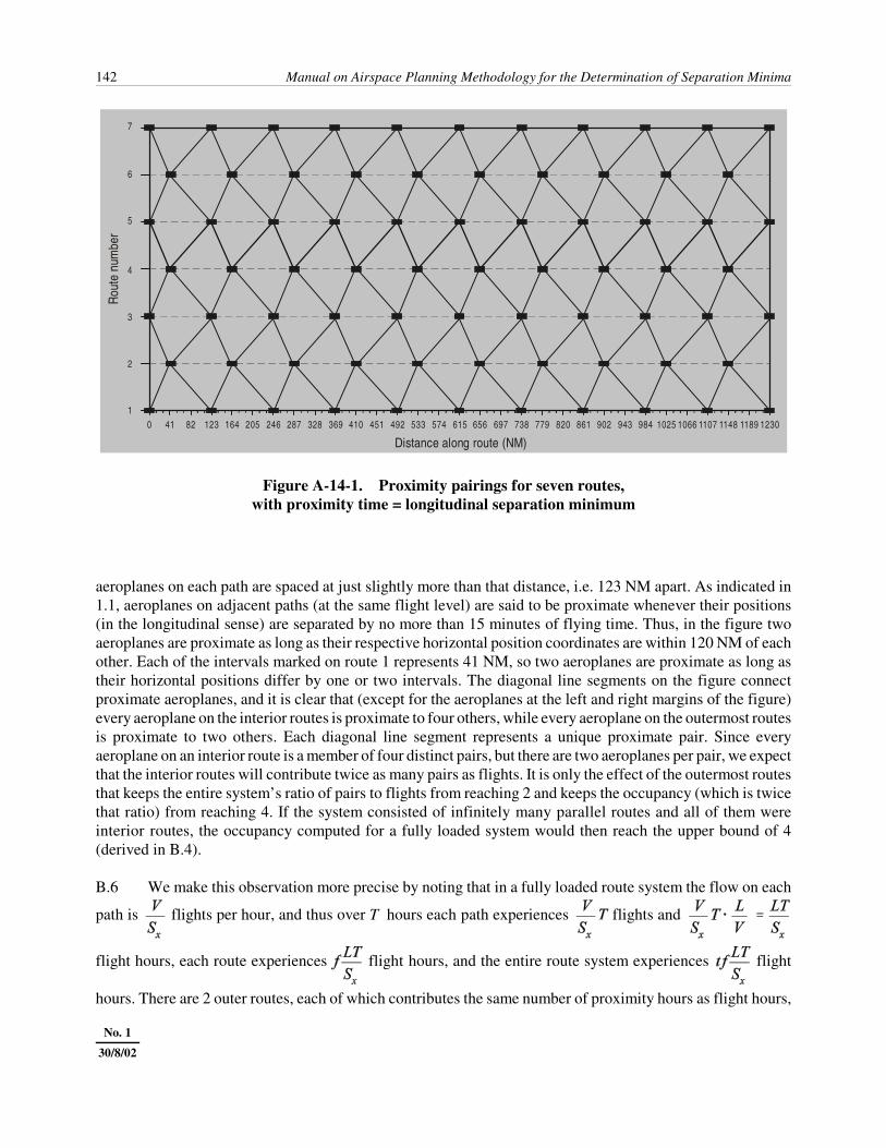
142 Manual on Airspace Planning Methodology for the Determination of Separation Minima
No. 1
30/8/02
0 41 82 123 164 205 246 287 328 369 410 451 492 533 574 615 656 697 738 779 820 861 902 943 984 1025 1066 1107 1148 1189 12301
2
3
4
5
6
7Ro
ute
num
ber
Distance along route (NM)
Figure A-14-1. Proximity pairings for seven routes,with proximity time = longitudinal separation minimum
aeroplanes on each path are spaced at just slightly more than that distance, i.e. 123 NM apart. As indicated in1.1, aeroplanes on adjacent paths (at the same flight level) are said to be proximate whenever their positions(in the longitudinal sense) are separated by no more than 15 minutes of flying time. Thus, in the figure twoaeroplanes are proximate as long as their respective horizontal position coordinates are within 120 NM of eachother. Each of the intervals marked on route 1 represents 41 NM, so two aeroplanes are proximate as long astheir horizontal positions differ by one or two intervals. The diagonal line segments on the figure connectproximate aeroplanes, and it is clear that (except for the aeroplanes at the left and right margins of the figure)every aeroplane on the interior routes is proximate to four others, while every aeroplane on the outermost routesis proximate to two others. Each diagonal line segment represents a unique proximate pair. Since everyaeroplane on an interior route is a member of four distinct pairs, but there are two aeroplanes per pair, we expectthat the interior routes will contribute twice as many pairs as flights. It is only the effect of the outermost routesthat keeps the entire system’s ratio of pairs to flights from reaching 2 and keeps the occupancy (which is twicethat ratio) from reaching 4. If the system consisted of infinitely many parallel routes and all of them wereinterior routes, the occupancy computed for a fully loaded system would then reach the upper bound of 4(derived in B.4).
B.6 We make this observation more precise by noting that in a fully loaded route system the flow on each
path is flights per hour, and thus over T hours each path experiences flights and
flight hours, each route experiences flight hours, and the entire route system experiences flight
hours. There are 2 outer routes, each of which contributes the same number of proximity hours as flight hours,

Appendix 14. Estimating occupancy and the rate of accidents due to the loss of plannedlateral separation for the individual components of a system of parallel routes 143
No. 1
30/8/02
and there are t�2 interior routes, each of which contributes twice as many proximity hours as flight hours.
Therefore, the system exhibits a total of proximity hours and an occupancy of
.
As t (the number of routes) increases, the occupancy approaches 4 from below.
B.7 In B.3 we found that Ey, the route system’s occupancy, is
.
If the system consists of exactly two routes, i.e. if t = 2, we can rewrite the occupancy as
.
For each flight level j, is greater than or equal to each of the flows and , and so
and . Therefore, each of the sums in the denominator is greater than or equal to the
numerator, whence the entire quotient is less than or equal to 1/2, and Ey is less than or equal to 4 � (1/2) = 2.
B.8 Figure A-14-2 is similar to Figure A-14-1, but depicts only two heavily loaded routes. As inFigure A-14-1, each diagonal line segment represents a unique proximate pair of aeroplanes. It is clear from thefigure that each aeroplane belongs to two pairs, while each pair consists of two aeroplanes, so except for anextra aeroplane shown at one or the other margin, the number of pairs equals the number of flights. Thus, ina maximally loaded system of two routes, we expect the ratio of pairs to flights to equal 1, and the occupancy,Ey, to equal 2. Note that the formula derived at the end of B.6 remains valid when t = 2, since it gives Ey = 4 �(4/2) = 4 – 2 = 2.
B.9 The NAT OTS proximity criterion of 15 minutes was probably chosen prior to 1981 when 15 minuteswas the minimum longitudinal separation in that route system. However, since 1981 the NAT OTS has used10 minutes as its longitudinal minimum, and thus the maximum possible flow on any of its paths has increased
from four aircraft per hour to six aircraft per hour. In the notation used above, hours corresponds to the

144 Manual on Airspace Planning Methodology for the Determination of Separation Minima
No. 1
30/8/02
15-minute separation minimum, and so the 10-minute minimum can be written as hours, and the
corresponding maximum flow rate as its reciprocal, (flights) per hour. Following the method in B.3 and
B.4, we recall that
Ey
.
We then note that for all i = 2, ..., t and all j = 1, ..., f , and so the second sum in the denominator,
is greater than or equal to the numerator, . A fortiori, the entire denominator
is greater than or equal to the numerator, whence the quotient is less than or equal to 1, and Ey � 6.
B.10 Figure A-14-3 illustrates a single flight level in a system of three heavily loaded parallel routes. (Moreroutes would have been depicted if the software used to prepare the figure had been capable of showing them).In this case each interval marked along route 1 represents 27 NM, and consecutive aeroplanes on each path arelongitudinally separated by three such intervals, i.e. by 81 NM, which is just slightly greater than the distance(of 80 NM) corresponding to the minimum separation of 10 minutes. Since the proximity criterion remains15 minutes of flying time (which corresponds to 120 NM), aeroplanes on adjacent routes are proximate if theirlongitudinal position coordinates are separated by one, two, three or four intervals, i.e. by 27, 54, 81 or 108 NM.As in Figures A-14-1 and A-14-2, the diagonal line segments connect proximate pairs, and it is clear from thefigure that every aeroplane on the interior route is proximate to six others, while every aeroplane on the outerroutes is proximate to three others. Since each interior route contributes six pairs per aeroplane, but every pairconsists of two aeroplanes, the interior routes contribute three times as many pairs as flights. Again, it is onlythe influence of the outermost routes that keeps the occupancy from reaching its theoretical maximum of 2 � 3= 6.
B.11 If the system consists of just two routes (i.e. if t = 2), we can rewrite the occupancy derived in B.9 as
Ey .

Appendix 14. Estimating occupancy and the rate of accidents due to the loss of plannedlateral separation for the individual components of a system of parallel routes 145
No. 1
30/8/02
0 41 82 123 164 205 246 287 328 369 410 451 492 533 574 615 656 697 738 779 820 861 902 943 984 1025 1066 1107 1148 1189 12301
2
3
4
5
6
7Ro
ute
num
ber
Distance along route (NM)
Figure A-14-2. Proximity pairings for two routes,with proximity time = longitudinal separation minimum
0 27 54 81 108 135 162 189 216 243 270 297 324 351 378 405 432 459 486 513 540 567 594 621 648 675 702 729 756 783 8101
2
3
4
5
6
7
Rout
e nu
mbe
r
Distance along route (NM)
Figure A-14-3. Proximity pairings for three routes,with proximity time = 1.5 × longitudinal separation minimum

146 Manual on Airspace Planning Methodology for the Determination of Separation Minima
No. 1
30/8/02
0 27 54 81 108 135 162 189 216 243 270 297 324 351 378 405 432 459 486 513 540 567 594 621 648 675 702 729 756 783 8101
2
3
4
5
6
7Ro
ute
num
ber
Distance along route (NM)
Figure A-14-4. Proximity pairings for two routes,with proximity time = 1.5 × longitudinal separation minimum
For each flight level j, is greater than or equal to each of the flows and , and so
and Therefore, each of the sums in the denominator is greater than
or equal to the numerator, whence the entire quotient is less than or equal to 1/2, and Ey is less than or equal to6 � (1/2) = 3.
B.12 Figure A-14-4 is similar to Figure A-14-3, but illustrates a system of just two routes. It is clear fromthe figure that each aeroplane belongs to three pairs, while each pair consists of two aeroplanes, so except foran extra aeroplane shown at one or the other margin, the number of pairs equals 3/2 the number of flights. Thus,in a fully loaded system of two routes, in which the proximity criterion is 3/2 the minimum longitudinalseparation, the ratio of proximity time to flight time is expected to equal 3/2, and the occupancy, Ey, to equal 3.
B.13 Paragraphs B.9 through B.12 demonstrate the effect of using a proximity criterion, , that is 3/2 of
the longitudinal separation minimum. More generally, it is clear that another ratio could be substituted for 3/2,and the arguments used in B.9 and B.11 would then yield maximum occupancy values corresponding to thatparticular ratio. Indeed, let q denote the ratio of proximity criterion to longitudinal separation minimum.Replacing the factor 3/2 by q, in B.9 and B.11, and repeating the arguments of those paragraphs, we find that4q is an upper bound on the occupancy of all multi-route systems, and 2q is an upper bound on the occupancyof systems that consist of exactly two routes.

Appendix 14. Estimating occupancy and the rate of accidents due to the loss of plannedlateral separation for the individual components of a system of parallel routes 147
No. 1
30/8/02
B.14 Imagine (as in B.6) a fully loaded route system in which the proximity time, , divided by the
separation minimum, equals q. Then the separation minimum is hours, and the traffic flow on each path
is its reciprocal, (flights) per hour. Thus, over T hours, each path experiences flights and
flight hours, each route experiences flight hours, and the entire route system
experiences flight hours. Since there are q separation intervals per proximity interval, every aeroplane
in the system is (on average) proximate to q aeroplanes on each of the routes adjacent to its own. Thus everyaeroplane on an interior route is proximate to 2q others, and every aeroplane on the two outermost routes isproximate to q others. Each of the t�2 interior routes therefore contributes 2q proximity hours per flight hour,while the two outer routes contribute q proximity hours per flight hour. Thus the system exhibits a total of
proximity hours
and an occupancy of
.
As t increases, this expression approaches 4q from below, and when t = 2, the expression simplifies to 2q. Thus,
in general, the least upper bound for the occupancy of a t-route system is .

Appendix 15NAVIGATION PERFORMANCE REQUIREMENTS FOR THE
INTRODUCTION OF 30 NM LATERAL SEPARATIONIN OCEANIC AND REMOTE AIRSPACE
1. INTRODUCTION
This appendix presents a method for estimating the risk of collision due to the loss of planned lateral separationin a system of parallel routes having 30 NM between adjacent routes. It considers several different systems ofparallel routes and, for each system, derives a navigational performance requirement that must be met in orderfor the system to operate with no more than the internationally accepted target level of safety (TLS) of 5 × 10�9
accidents per flight hour. In order to eliminate unnecessary verbiage, this appendix does not repeatedly statethat such accidents are due to the loss of planned lateral separation. Unless the text specifically refers to the lossof another form of separation, all mention of accidents, accident rates or collision rates refers to those causedby the loss of planned lateral separation.
2. A LIMIT ON TYPICALNAVIGATIONAL ERRORS
2.1 In establishing standard values of required navigation performance (RNP) for aeroplanes using oceanicroute systems, the RGCSP considered the probability that aeroplanes assigned to adjacent parallel routes havelaterally overlapping positions. This lateral overlap probability, which is a major determinant of a routesystem’s accident rate, varies with the navigational accuracy of the fleet using the system, and the navigationalaccuracy can be characterized by a limit on 95 per cent of the typical lateral errors experienced by the fleet’saeroplanes. In examining the functional dependence of lateral overlap probability on this “95 per centcontainment limit”, the RGCSP observed that over a fairly large range of values, reductions in the containmentlimit lead to significant reductions in the overlap probability. However, once the containment limit decreasesto approximately one-sixth of the separation between the routes, further decreases yield only negligibly smallreductions in overlap probability. Thus, if an airspace management authority wishes to establish an RNP forthe fleet using a system of parallel routes, it should not ask operators to exhibit better lateral performance thanthat which produces a 95 per cent containment limit equal to one-sixth of the separation.
2.2 In order to avoid a proliferation of RNP standards, the RGCSP initially established only two suchstandards for oceanic flight, RNP 20 and RNP 12.6. It later added RNP 10. For en-route flights over continentalairspace, the RGCSP adopted RNP 1, RNP 4 and, for a portion of European airspace, RNP 5.
No. 1 14830/8/02

Appendix 15. Navigational performance requirements for the introduction of 30 NM lateral separation in oceanic and remote airspace 149
No. 1
30/8/02
2.3 In recent years some airspace management authorities have expressed an interest in establishing oceanicroute systems having 30 NM between adjacent parallel routes. In order for such a system to operate safely, itsfleet needs to exhibit lateral performance equivalent to (or better than) RNP 5. However, it is also importantto remember that many aeroplanes approved for RNP 5 in continental airspace may not be able to operate atthat accuracy in oceanic airspace because their RNP 5 performance may depend on the use of ground-basednavigation aids (NAVAIDS). In recent years many new long-range aeroplanes (such as those equipped withBoeing’s “FANS-1” package) have been granted RNP 4 approvals, and it is likely that those aeroplanes willbe the first to operate on oceanic route systems having 30 NM separation between adjacent parallel routes.
3. LIMITS ON THE RATE OFATYPICAL LATERAL ERRORS
3.1 In the present section several possible configurations of parallel routes are examined. For eachconfiguration a representative set of occupancies (occupancy being a measure of exposure to risk) ranging from0 to 2 is considered. For each occupancy the maximum tolerable rate of atypical lateral errors correspondingto the TLS of 5 × 10�9 accidents per flight hour is computed. The accident rate is estimated by applying thewell-known Reich model for parallel routes, and in so doing the model’s traditional notation is used. Themeanings of the model’s parameters are shown in Table A-15-1, as are values typical of one particular oceanicairspace in the mid- to late 1990s. It is important to remember that fleet characteristics vary from one airspaceto another and also change over time. Similar computations for another airspace should use the parameter valuesexpected to prevail there during the time period in which the relevant separation is to be applied.
In the simplest cases, involving two flight paths at the same altitude, the Reich model gives the accident rate
as accidents per flight hour when the routes carry traffic in the same direction
and as accidents per flight hour when the routes carry traffic in opposite
directions.
3.2 As was noted above, the lateral overlap probability, Py(S)y, varies significantly with typical navigationalaccuracy when the 95 per cent containment limit exceeds one-sixth of the separation between the routes beingconsidered. When the containment limit is less than a sixth of Sy, the lateral overlap probability becomes nearlyconstant with respect to typical navigational accuracy, but it does vary (almost) linearly with �, the fleet’s rateof atypical lateral errors.
3.3 Analysts generally use a double double exponential (DDE) density function to characterize a fleet’slateral errors so that they can thereby describe both typical and atypical errors. The DDE function is oftenwritten in the form
.
It is thus a weighted sum of two double exponential densities (also called DE or “first Laplace” densities), the

150 Manual on Airspace Planning Methodology for the Determination of Separation Minima
No. 1
30/8/02
first of which describes typical errors, and the second of which describes atypical errors. Each of the parameters
and is times the standard deviation of its respective DE density. The weighting parameter � is the
proportion of time during which an “average” aeroplane is committing an atypical error.
3.4 We consider a pair of parallel routes separated by Sy NM and assume that the lateral errors of theaeroplanes using both routes can be characterized by the same DDE density function f. If we randomly selecttwo aeroplanes, one from those assigned to each route, then Py(Sy), the probability that the two chosenaeroplanes are in lateral overlap, is approximately
Of the three terms enclosed in rectangular brackets in this expression for Py(Sy), the first (describing “core-coreinteraction”) dominates when the 95 per cent containment limit of the fleet’s typical errors exceeds Sy/5. Whenthe 95 per cent containment limit is less than Sy/6, the third term (describing “core-tail interaction”) dominates,generally contributing more than 99 per cent of the value of Py(Sy).
3.5 After choosing a value of same-direction or opposite-direction occupancy, we apply the appropriateformula from the end of 3.1 to derive the value of � at which Py(Sy) is small enough for the accident rate toequal the TLS. In other words, when the routes carry traffic in the same direction, we find the value of � atwhich
,
and when they carry traffic in opposite directions, the value of � is found at which
.
Using the constants given in Table A-15-1, we find that when the routes carry traffic in the same direction, we
seek the value of � for which , and when they carry traffic in opposite directions, we seek
the value of � for which .
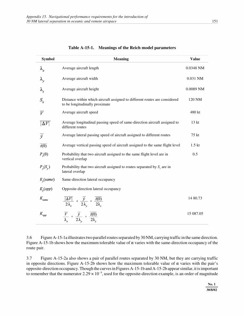
Appendix 15. Navigational performance requirements for the introduction of 30 NM lateral separation in oceanic and remote airspace 151
No. 1
30/8/02
Table A-15-1. Meanings of the Reich model parameters
Symbol Meaning Value
Average aircraft length 0.0348 NM
Average aircraft width 0.031 NM
Average aircraft height 0.0089 NM
Distance within which aircraft assigned to different routes are consideredto be longitudinally proximate
120 NM
Average aircraft speed 480 kt
Average longitudinal passing speed of same-direction aircraft assigned todifferent routes
13 kt
Average lateral passing speed of aircraft assigned to different routes 75 kt
Average vertical passing speed of aircraft assigned to the same flight level 1.5 kt
Probability that two aircraft assigned to the same flight level are invertical overlap
0.5
Probability that two aircraft assigned to routes separated by Sy are inlateral overlap
Same-direction lateral occupancy
Opposite-direction lateral occupancy
14 80.73
15 087.05
3.6 Figure A-15-1a illustrates two parallel routes separated by 30 NM, carrying traffic in the same direction.Figure A-15-1b shows how the maximum tolerable value of � varies with the same-direction occupancy of theroute pair.
3.7 Figure A-15-2a also shows a pair of parallel routes separated by 30 NM, but they are carrying trafficin opposite directions. Figure A-15-2b shows how the maximum tolerable value of � varies with the pair’sopposite-direction occupancy. Though the curves in Figures A-15-1b and A-15-2b appear similar, it is importantto remember that the numerator 2.29 × 10�9, used for the opposite-direction example, is an order of magnitude

152 Manual on Airspace Planning Methodology for the Determination of Separation Minima
No. 1
30/8/02
30 NM
Figure A-15-1a. A pair of parallel routescarrying traffic in the same direction
0 0.2 0.4 0.6 0.8 1 1.2 1.4 1.6 1.8 2
0.00035
0.0003
0.00025
0.0002
0.00015
0.0001
5E-05
0
Alph
a
Same-direction occupancy
Route separation = 30 NMTLS = 5E-9
Figure A-15-1b. Maximum acceptable value of alpha
smaller than the numerator 2.33 × 10⁻⁸ used for the same-direction case, and so the maximum tolerable values

Appendix 15. Navigational performance requirements for the introduction of 30 NM lateral separation in oceanic and remote airspace 153
No. 1
30/8/02
30 NM
Figure A-15-2a. A pair of parallel routescarrying traffic in the opposite direction
0 0.2 0.4 0.6 0.8 1 1.2 1.4 1.6 1.8 2
3.5E-05
3E-05
2.5E-05
2E-05
1.5E-05
1E-05
5E-06
0
Alph
a
Opposite-direction occupancy
Route separation = 30 NMTLS = 5E-9
Figure A-15-2b. Maximum acceptable value of alpha

154 Manual on Airspace Planning Methodology for the Determination of Separation Minima
No. 1
30/8/02
of � shown in Figure A-15-2b are an order of magnitude smaller than the corresponding values shown inFigure A-15-1b. In particular, note that the scales of the vertical axes in the two figures differ by an order ofmagnitude. (When the fleet using the route system exhibits typical lateral errors whose 95 per cent containmentvalue is less than Sy/6, Py(Sy) varies (almost) directly with �. As was shown in 3.5, Py(Sy) varies inversely withoccupancy. Thus we expect � also to vary inversely with occupancy, and indeed Figures A-15-1b and A-15-2bboth look like hyperbolas of the form constant/x.)
3.8 The computations of maximum acceptable values of � assume that the fleet’s typical performance justsatisfies RNP 4. Thus 95 per cent of typical lateral deviations are assumed to be less than 4 NM. It follows thatthe parameter �1 has the value 4/[�ln(.05)] = 1.3352. The parameter �2 is taken to equal Sy, the distance betweenthe routes — i.e. 30 NM. This is a conservative value in that it maximizes the lateral overlap probability Py(Sy).
3.9 Figure A-15-3a shows four parallel routes, with traffic moving in the same direction on all of them. Forease of reference, the routes are labelled consecutively as R1, R2, R3 and R4. We assume three flight levels inthis example, and we assume a traffic distribution in which the lowest flight level carries 1/4 of the traffic, themiddle level carries 5/12 of it, and the upper level carries the remaining 1/3. On each flight level, R1 carries1/12 of the traffic, R2 carries 1/3 of it, R3 carries 5/12 of it, and R4 carries the remaining 1/6. Thus the examplereflects a concentration of traffic on the system’s central routes, as is sometimes observed in practice.
3.10 Appendix 14 derives formulae for the occupancies and accident rates of all pairs of flight paths in sucha system, as well as for collections of pairs of flight paths. Figure A-15-3b is based on an analysis that firstapplies the formulae of that appendix to compute accident rates, and then varies �, the rate of atypical errors,to find the value that produces an accident rate equal to the TLS of 5 × 10�9 accidents per flight hour. The figureshows the values of � corresponding to (adjacent flight path) occupancies ranging from 0.1 to 2.0. The analysissupporting Figure A-15-3b differs from most estimates of accident rates (such as those on whichFigures A-15-1b and A-15-2b are based) in that it includes not only the rate of accidents due to the loss ofplanned separation between aeroplanes assigned to adjacent routes, but also the rate of accidents fromaeroplanes assigned to non-adjacent routes. In the example used to generate Figure A-15-3b, the inclusion ofnon-adjacent routes increases the accident rate by almost a seventh and reduces the maximum acceptable � byalmost 13 per cent. The example suggests that while accident rates generated from non-adjacent routesconstitute a minor contribution to the total rate, that contribution is still far from being negligible orinsignificant.
3.11 The analysis mentioned in 1.1 was based on a system of seven parallel routes operating on seven flightlevels. It was modelled after the North Atlantic Organized Track System (NAT OTS) as it operated in the mid-1990s, prior to the implementation of a reduced vertical separation minimum (RVSM) of 1 000 feet. An earlierattempt to estimate the maximum acceptable values of � in such a system, discussed at the spring 1995 meetingof RGCSP WG/A, had even attempted to account for the concentration of traffic on the system’s central routesand central flight levels, but its analysis of the effect of the concentration was not correct. Applying the resultsof Appendix 14 is expected to remedy the errors of the earlier analyses.
3.12 Figure A-15-4 graphs the results of an analysis similar to the one that supports Figure A-15-3b. Weassume a system of seven parallel routes on seven flight levels, and we take the distribution of traffic on theindividual flight paths to be the distribution observed for eastbound NAT OTS traffic on 15 August 1994 (thesame distribution used in the spring 1995 analysis). The maximum acceptable values of � shown inFigure A-15-4 are somewhat smaller than the corresponding values shown in Figure A-15-3b, which arethemselves somewhat smaller than those shown in Figure A-15-1b. In the analysis supporting Figure A-15-4,

Appendix 15. Navigational performance requirements for the introduction of 30 NM lateral separation in oceanic and remote airspace 155
No. 1
30/8/02
30 NM
30 NM
30 NM
R1
R2
R3
R4
Figure A-15-3a. Four parallel routes carrying trafficin the same direction
we find that the rate of accidents due to collisions between aeroplanes assigned to (co-altitude) adjacent flightpaths constitutes slightly more than 75 per cent of the total accident rate. Aeroplanes assigned to paths separatedby twice the minimum lateral separation account for another 20 per cent of the total; those assigned to pathsseparated by three times the minimum distance contribute more than 4 per cent; and those assigned to pathsseparated by four times the minimum distance contribute most of the remaining 1 per cent. Thus it can onceagain be seen that aeroplanes assigned to non-adjacent paths make a significant contribution — nearly 25 percent in this case — to the route system’s total accident rate.
3.13 Recall that the RNP of the airspace determines the parameter �1 of the DDE density function and thatwe have assumed the most conservative value for the parameter �2. The analyses supporting Figures A-15-1b,2b, 3b, and 4 derive the maximum tolerable values of �, the rate of atypical lateral errors, under which the givenroute systems and occupancies can satisfy the TLS of 5 × 10�9 accidents per flight hour. The three parameters,�, �1 and �2, completely determine the DDE density function used to describe aircraft performance that justmeets the TLS.
3.14 The North Atlantic (NAT) minimum navigation performance specification (MNPS) also states aircraftperformance requirements in terms of three parameters. The first of them is a limit on the standard deviationof lateral track-keeping errors. The second, usually denoted �, is a limit on the proportion of total flight time
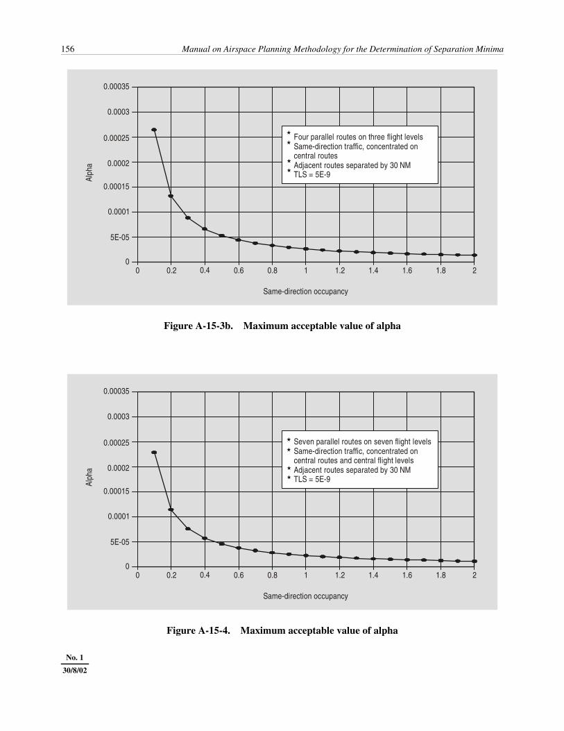
156 Manual on Airspace Planning Methodology for the Determination of Separation Minima
No. 1
30/8/02
0 0.2 0.4 0.6 0.8 1 1.2 1.4 1.6 1.8 2
0.00035
0.0003
0.00025
0.0002
0.00015
0.0001
5E-05
0
Alph
a
Same-direction occupancy
Four parallel routes on three flight levelsSame-direction traffic, concentrated oncentral routesAdjacent routes separated by 30 NMTLS = 5E-9
�
�
�
�
Figure A-15-3b. Maximum acceptable value of alpha
0 0.2 0.4 0.6 0.8 1 1.2 1.4 1.6 1.8 2
0.00035
0.0003
0.00025
0.0002
0.00015
0.0001
5E-05
0
Alph
a
Same-direction occupancy
Seven parallel routes on seven flight levelsSame-direction traffic, concentrated oncentral routes and central flight levelsAdjacent routes separated by 30 NMTLS = 5E-9
�
�
�
�
Figure A-15-4. Maximum acceptable value of alpha

Appendix 15. Navigational performance requirements for the introduction of 30 NM lateral separation in oceanic and remote airspace 157
No. 1
30/8/02
spent more than half of a separation standard away from the route centre line, i.e. a limit on the rate of grosslateral errors. The third, called �, is a limit on the proportion of flight time spent in the immediate vicinity ofan adjacent route’s centre line. In the MNPS, the “immediate vicinity” is taken to mean the 20-NM-wide bandthat covers all points within 10 NM of the centre line. In the present analysis, for which adjacent routes haveonly 30 NM separation between their centre lines, the “immediate vicinity” is taken to mean the 12-NM-wideband covering all points within 6 NM of the adjacent route’s centre line. Fortunately, it is not difficult totranslate values of �, �1 and �2 into corresponding values of the three parameters used in the NAT MNPS. Thelimit on the standard deviation of lateral track-keeping errors is logically equivalent to an RNP, and values for� and � can be obtained by integrating the DDE density function over appropriate intervals or, equivalently,by computing differences of the DDE distribution function evaluated at appropriate points.
3.15 The NAT MNPS requires typical navigation equivalent to RNP 12.6, while (as indicated above) asystem having a 30 NM lateral separation minimum is likely to operate with RNP 4. Table A-15-2 shows thevalues of � that are graphed in Figure A-15-4 (i.e. the maximum tolerable rates of atypical errors for a one-wayroute system that has seven routes and seven flight levels, has a minimum lateral separation of 30 NM andtypically has a traffic distribution resembling that of the eastbound NAT OTS on 15 August 1994).Table A-15-2 also shows the � and � values corresponding to each value of �. Even at the lowest occupancyshown in the table, i.e. at 0.1, these � and � values are considerably more stringent than the values given in theNAT MNPS, where � = 5.3 × 10�4 and � = 1.3 × 10�4.
4. MEANS OF REDUCING THE RATE OFGROSS LATERAL ERRORS
Several improvements in avionics, communication systems and air traffic control systems that were to beimplemented during the late 1990s were expected to significantly reduce the rate of gross lateral errors andthereby enable reductions in lateral separations. In order to determine whether the proposed systems did indeedhave the potential to eliminate oceanic gross errors, researchers from the United States Federal AviationAdministration’s Flight Standards Service carefully examined each of the “Table A” and “Table B” errorsentered into the database of the North Atlantic Central Monitoring Agency (NAT CMA) between 1986 and1993. Their examination revealed that the proposed improvements had the potential to eliminate approximately95 per cent of the listed gross errors. While this result confirmed the potential benefit of pursuing the proposedimplementations, it will be necessary to confirm that the various subsystems which are intended to contributeto error reduction actually operate as planned. It is also worth noting that any new system has the potential tocause previously unforeseen errors, and since some of the new systems are highly complex, it may be extremelydifficult to determine the causes of such errors.
5. APPLICATION CONSIDERATIONS
5.1 Each oceanic airspace has characteristics that distinguish it from others, such as the number and lengthof its routes, and the dimensions, speeds, and navigational characteristics of the aeroplanes that use it. Thequantitative results reported in section 3 are derived from typical values of the parameters that are significantin collision risk analyses, but they should not be viewed as applicable to all oceanic airspace. Nonetheless, itwould not be difficult to replicate those analyses with the values found to be applicable to any particular routesystem.

158 Manual on Airspace Planning Methodology for the Determination of Separation Minima
No. 1
30/8/02
Table A-15-2. Eta and zeta values computed fromdouble double exponential (DDE) distribution function
Lambda1 = 1.3352Lambda2 = 30
Half lambda2 =Half separation = 15
Outer zeta limit = 36
Inner zeta limit = 24
Occupancy Maximum alpha Eta Zeta
0.1 2.29E-04 1.52E-04 3.40E-050.2 1.15E-05 8.27E-05 1.70E-050.3 7.53E-05 5.95E-05 1.13E-050.4 5.72E-05 4.79E-05 8.50E-060.5 4.58E-05 4.10E-05 6.80-060.6 3.82E-05 3.64E-05 5.67-060.7 3.27E-05 3.30E-05 4.86-060.8 2.86E-05 3.06E-05 4.25-060.9 2.54E-05 2.86E-05 3.78-061.0 2.29E-05 2.71E-05 3.40-061.1 2.08E-05 2.58E-05 3.10-061.2 1.91E-05 2.48E-05 2.84-061.3 1.76E-05 2.39E-05 2.62-061.4 1.63E-05 2.31E-05 2.43-061.5 1.52E-05 2.25E-05 2.27-061.6 1.43E-05 2.19E-05 2.13-061.7 1.34E-05 2.14E-05 2.01-061.8 1.27E-05 2.09E-05 1.89-061.9 1.20E-05 2.05E-05 1.80-062.9 1.14E-05 2.01E-05 1.71-06
5.2 Appropriate values for some of the parameters used in collision risk analyses can be gathered throughsurveys of operators; others can be found through examinations of radar-reported aircraft positions; still othersmay be obtained from careful sorting of the data recorded on flight-progress strips. While some of the processesinvolved in determining parameter values are labour-intensive and may require weeks or months of effort, mostcan be accomplished within a reasonable time period. Gross errors, however, occur quite infrequently, and thusan airspace management authority that wishes to determine whether its route system’s gross-error rate isacceptably low may need to monitor the system over a period of several years and establish a database such as

Appendix 15. Navigational performance requirements for the introduction of 30 NM lateral separation in oceanic and remote airspace 159
No. 1
30/8/02
that of the NAT CMA. Of course, if the database is not well-maintained — in particular, if it does not includeall of the gross errors that occur in the airspace — then the authority may mistakenly conclude that its routesystem can operate safely with smaller separations than are warranted by the system’s true (but unknown) rateof gross errors.
6. CONCLUSION
Section 3 considers four different examples of route systems having a 30 NM separation between adjacent co-altitude flight paths. For each of those systems, it derives the maximum rate of atypical errors that can betolerated for each level of occupancy if the system is to meet a TLS of 5 × 10�9 accidents per flight hour.

Appendix 16A METHOD OF DERIVING PERFORMANCE
STANDARDS FOR AUTOMATIC DEPENDENTSURVEILLANCE (ADS) SYSTEMS
1. INTRODUCTION
An airspace management authority planning to implement an ADS system may wish to establish performancestandards for the system before it embarks upon the preparation of detailed specifications and other procurementdocuments. This appendix suggests a procedure for obtaining five significant performance standards:
pw — the minimum acceptable probability that the system prevents a waypoint-insertion lateralerror;
pn — the minimum acceptable probability that the system prevents a preventable non-waypoint-insertion lateral error;
P(A) — the minimum acceptable probability that the sequence of actions referred to in thisappendix as an “ADS cycle” is completed;
t — a maximum acceptable time for completion of an ADS cycle; and
m — the minimum acceptable probability that an ADS cycle is completed in time t, given thatit is completed.
The procedure is based on two important characteristics of ADS systems: their operation of route conformancefunctions and their use of event contracts.
2. OBTAINING VALUES OF pw AND pn
2.1 The first step in the procedure assumes that the airspace management authority maintains (or hasaccess to) a monitoring system that records the gross lateral errors committed by the fleet of aeroplanes that useits routes. For example, the Central Monitoring Agency (CMA) of the United Kingdom’s National Air TrafficServices maintains statistics on the performance of the North Atlantic fleet; the United States Federal AviationAdministration’s Asia-Pacific Approvals Registry and Monitoring Organization (APARMO) performs a similarfunction for the Pacific fleet; and Spain’s Aena operates the South Atlantic Monitoring Agency (SATMA).Although the monitoring system may be employed for various other purposes, the procedure described here ischiefly concerned with its ability to determine a route system’s rate of gross lateral errors r. One would usuallyexpect r to be derived empirically and to describe a prevailing rate, but in some contexts it might indicate
No. 1 16030/8/02

Appendix 16. A method of deriving performance standards for automatic dependentsurveillance (ADS) systems 161
No. 1
30/8/02
an expected future rate, as long as its value could be justified on reasonable analytic grounds. The rate r mightbe low enough to permit safe operations under current conditions, but be too high for the route system to operatesafely after the implementation of a projected change, such as a reduction in the lateral separation betweenadjacent parallel routes. The implementation of ADS might be needed in order to reduce the gross error rateto an acceptable level.
2.2 Thus the airspace management authority also needs to select a maximum tolerable gross error rate�R. �R is the maximum tolerable probability that after the implementation of ADS a randomly chosen flightis committing a gross error.
2.3 An examination of gross error data, such as those maintained by the CMA, may suggest a rate of errorsattributable to failures of navigation systems. It is reasonable to expect that whenever air traffic controllers arenot informed of such a failure, the crew of the affected aeroplane is also unaware of it for, in most cases, if thecrew were aware of it, it would notify its servicing ATC unit. If the flight crew has not been informed of afailure, then the navigation system itself, and all aircraft subsystems with which it communicates, must havebeen unable to detect the failure. The CMA normally requests an investigation of each NAT gross lateral errorthat comes to its attention, and it retains a record of the cause of the error. If other monitoring agencies dolikewise, then a typical airspace management authority should have access to data that will enable it to estimatethe fraction, fu, of all gross lateral errors in its airspace caused by undetectable failures of navigation systems.Since airborne ADS units cannot detect these failures, the ADS system will be unable to prevent the resultingerrors, and the fleet’s rate of errors after the implementation of ADS will be at least rfu. If rfu > �R, then theimplementation of ADS will not by itself be capable of reducing the system’s gross error rate to an acceptable
level. The remainder of this appendix therefore applies only to values of fu less than , i.e. values for which
rfu < �R.
2.4 It has been observed that, in recent years, in at least one heavily travelled airspace, a large proportionof gross lateral errors have been waypoint-insertion errors. Using data from the relevant monitoring agency, theauthority can also estimate fw , the fraction of all gross errors that are waypoint-insertion errors. The routesystem’s fraction of detectable, and possibly preventable, gross errors is 1 � fu. Since all waypoint-insertion
errors are candidates for prevention by ADS, it is clear that fw < 1 � fu , and that is the fraction of possibly
preventable errors that are waypoint-insertion errors. Thus is the fraction of possibly
preventable gross errors that are non-waypoint-insertion errors. The underlying rate of (preventable) waypoint-insertion gross errors is rfw , and the underlying rate of preventable non-waypoint-insertion gross errors isr(1 � fu � fw). That is, prior to ADS implementation, rfw = P(a randomly chosen flight is committing a waypoint-insertion gross error); likewise, r(1 � fu � fw) = P(a randomly chosen flight is committing a preventable non-waypoint-insertion gross error). To save space, let the abbreviation “WPIE” denote “waypoint-insertion grosserror”, and let “NWPIE” denote “non-waypoint-insertion gross error”.
2.5 The route conformance function of ADS (much of which is implemented in the ground-basedcomponent of the system) is expected to eliminate most WPIEs. Let pw = P(ADS prevents a WPIE), and let pn
= P(ADS prevents a preventable NWPIE). Then 1 � pw = P(ADS fails to prevent a WPIE) and 1 � pn = P(ADSfails to prevent a preventable NWPIE). After ADS is implemented in a route system, the maximum tolerablerate of gross errors is �R. However, ADS will not have any effect on the portion of the gross error rate
162 Manual on Airspace Planning Methodology for the Determination of Separation Minima
No. 1
30/8/02
represented by rfu, the rate of non-preventable gross errors. If the route system’s rate of gross errors after theimplementation is to meet the maximum tolerable rate �R, it must satisfy:
�R � P(a randomly chosen flight is committing a preventable gross error)
= P(a randomly chosen flight is committing a WPIE)
+ P(a randomly chosen flight is committing a preventable NWPIE)
= P(ADS fails to prevent a WPIE)rfw
+ P(ADS fails to prevent a preventable NWPIE)r(1 � fu � fw)
= (1 � pw)rfw + (1 � pn)r(1 � fu � fw).
Equivalently,
� (1�pw)fw + (1�pn)(1�fu�fw)
= fw � fw pw + 1 � fu � fw � (1�fu�fw)pn
= 1 � fu � fw pw � (1�fu�fw)pn
and
� 1 � fw pw � (1�fu�fw)pn .
Thus
(1�fu�fw )pn � 1 � � fw pw
or, equivalently,
pn � . (1)
From this inequality it is clear that the set of possible values of the probability pn is bounded from below by a
linear function of the probability pw . The line that forms the lower bound has pw-intercept and
pn-intercept . However, since pw and pn are probabilities, they also must lie between 0 and 1.

Appendix 16. A method of deriving performance standards for automatic dependentsurveillance (ADS) systems 163
No. 1
30/8/02
1
0.8
0.6
0.4
0.2
0.20
0 0.4 0.6 0.8 1
η-5
ff
u
w
= 0.05 = 0.9
R = 1.41•10 6.4•10
-5
r =feasiblevalues of
and p pw n
P n =
P(AD
S pr
even
ts a
pre
vent
able
NW
PIE)
pw = P(ADS prevents a WPIE)
Figure A-16-1. Relationship between required probabilities
2.6 Thus, once the authority has chosen values for the parameters �R, r, fu and fw, its choice of theprobabilities pw and pn is constrained by the linear bound given in inequality (1) and by the requirement that theyremain between 0 and 1. The area to the right of the sloping line in Figure A-16-1 illustrates a set of feasiblevalues of pn and pw . In this particular example, the parameters have the values �R = 1.41 � 10�5, r = 6.4 � 10�5,fu = 0.05 and fw = 0.90. Note that where pw is greater than or equal to 0.8663, pn can take any value between 0and 1 because the ADS route conformance function eliminates enough WPIEs that it is not necessary for ADSto eliminate any preventable NWPIEs in order to reduce the overall error rate to �R. On the other hand, wherepw is less than or equal to 0.8107, the route conformance function is unable to prevent enough waypoint errorsto reduce the overall error rate to �R, even if ADS completely eliminates all other preventable errors. Of course,different inputs would change the graph, but if it remained similar to Figure A-16-1, there is a substantialpossibility that the ADS route conformance function would suffice to reduce the overall gross error rate to therequired level because its success rate has been predicted to be better than 86.63 per cent.

164 Manual on Airspace Planning Methodology for the Determination of Separation Minima
No. 1
30/8/02
1
0.8
0.6
0.4
0.2
0.20
0 0.4 0.6 0.8 1
η-5
ff
u
w
= 0.05 = 0.9
R = 1.41•10 6.4•10
-5
r =
feasiblevalues of
and p pw n
p n =
P(AD
S pr
even
ts a
pre
vent
able
NW
PIE)
pw = P(ADS prevents a WPIE)
Figure A-16-2. Relationship between required probabilities
2.7 The boundary line in Figure A-16-1 is quite steep because fw, the fraction of gross errors that arewaypoint-insertion errors, is a large fraction (90 per cent) of the total. In other words, the overall rate of grosserrors is reduced by the required extent if and only if the rate of waypoint-insertion errors is reduced by nearlythe same extent. Even if all other gross errors are eliminated, it is still necessary to reduce waypoint-insertionerrors by 81.07 per cent, but if ADS eliminates 86.63 per cent of waypoint-insertion errors, it does not need toeliminate any others.
2.8 Figure A-16-2 shows an example in which fw = 0.5, a fraction typical of one heavily used airspaceduring the early 1990s. In this case, the lower right end of the boundary line shows that even if pw = 1 (i.e. ifADS prevents 100 per cent of waypoint-insertion errors) it still needs to prevent at least 62.14 per cent of otherpreventable errors in order to reduce the error rate to �R = 1.41�10�5. Likewise, the top left end of the boundaryline shows that if ADS can eliminate 100 per cent of preventable non-waypoint-insertion errors, then it will stillneed to prevent at least 65.93 per cent of waypoint-insertion errors in order to succeed in reducing the overallrate to �R.
2.9 Thus the authority can begin its specification of ADS performance parameters by:

Appendix 16. A method of deriving performance standards for automatic dependentsurveillance (ADS) systems 165
No. 1
30/8/02
a) estimating r, an underlying rate of gross lateral errors;
b) selecting a maximum tolerable probability, �R, that a typical flight will commit a gross lateralerror after the implementation of ADS;
c) estimating fu, the fraction of gross lateral errors that ADS cannot be expected to prevent (whilerecognizing that if rfu > �R, then the implementation of ADS will not, by itself, be capable ofreducing the system’s gross error rate to an acceptable level);
d) estimating fw, the fraction of gross lateral errors that are waypoint-insertion errors; and
e) using inequality (1) to select pw, the minimum acceptable probability that a waypoint-insertionerror will be prevented by ADS, and pn, the minimum acceptable probability that a (preventable)non-waypoint-insertion error will be prevented by ADS.
2.10 The very significant difference between Figures A-16-1 and A-16-2 (figures that reflect differentprevailing conditions in the same airspace during different time periods) illustrates an important principle.Different airspace, and even the same airspace operating in different time periods, can exhibit differentcharacteristics, and thus an analysis of safety requirements done for one of them is not necessarily relevant toanother. The airspace management authority must be careful to select parameter values that reflect the airspaceand the time period relevant to its planning.
3. MODELLING ADS OPERATION
3.1 A basic scenario
3.1.1 Having chosen or derived values for the parameters listed in 2.9, the airspace management authoritycan then derive a limit on the maximum acceptable time for the transmission of the sequence of messages usedby an ADS system and an associated communications link to prevent the occurrence of a gross lateral error. Theremainder of this section explains the model used to derive that limit.
3.1.2 ADS systems send aircraft positions to air traffic controllers when the aircraft are beyond the coverageof surveillance radar. An ADS system consists of both ground-based and airborne components and may alsoinclude a space-based communications link. The ground-based component typically arranges a “contract” withthe airborne component of each aeroplane that participates in the system, and that contract specifies the kindsof data that are to be reported, as well as the conditions under which reports are to be transmitted.
3.1.3 The messages sent by the airborne component generally incur transmission costs, and in order to keepsuch costs reasonably low, current ADS systems employ typical reporting rates of approximately one report per15 minutes. Such low update rates are clearly of very little use in promptly notifying the air traffic control(ATC) system of unauthorized or unintentional deviations from the aeroplane’s planned route of flight, sincethere is only a small probability that such a deviation occurs shortly before the airborne unit sends a scheduled

166 Manual on Airspace Planning Methodology for the Determination of Separation Minima
No. 1
30/8/02
report. Instead, the ADS system relies on the airborne unit to monitor its aircraft’s progress along its clearedroute of flight and to automatically report to the ATC system whenever the aeroplane deviates from that routeby more than some prescribed distance. In this discussion that distance is called B because it defines a buffer(of width 2B) about the route’s centre line. The angle by which the aeroplane’s true path deviates from the routeis denoted �d.
3.1.4 Suppose that an aeroplane begins to deviate from its cleared route of flight. (The present discussiondoes not address the issue of whether the deviation is appropriate or not. Some deviations result from humanerror or equipment malfunction. Others are intentional, and of those, some are obviously necessary to ensuresafety of flight.) When the aeroplane has laterally moved distance B from the centre line of its cleared route,the airborne ADS unit should recognize that it is passing beyond the buffer and should generate a report to theATC system. However, it is not unreasonable to imagine that the airborne ADS unit and the ground-based ATCsystem might have different definitions of the cleared route. Such an error could result from various causes, butregardless of the cause, the error could lead the airborne unit to understand that it is following the cleared route,even though its path is in fact diverging from that which the ATC system understands the cleared route to beand which it expects the aeroplane to be following. There are, undoubtedly, a variety of other means by whichthe airborne unit might fail to generate a report to the ATC system, such as failure of its electronic componentsor execution of faulty software. Whatever they may be, the existence of mechanisms that prevent the generationor transmission of such reports leads to the conclusion that while the probability of correctly generating andtransmitting a report may be relatively large, it must still be strictly less than 1. Let pt denote that probability.In the (highly probable) event that a report is transmitted, let T1 denote the random variable that is the timebetween the aeroplane’s passage out of the buffer and its transmission of the report.
3.1.5 The report typically passes through an elaborate, complex communications system consisting of manylinks. Let pd denote the probability that it reaches the correct ATC system, and in the event that it does so, letthe random variable D be the time from its transmission to its reception.
3.1.6 When the ADS report reaches the ATC system, it may be processed by a controller (perhaps aided bya computer), and the controller may respond by transmitting a message telling the pilot to return to the clearedroute of flight. Let pc denote the probability that the ATC system correctly generates and transmits such amessage, and in the event that it does so, let the random variable C be the time from the arrival of the ADSreport to the transmission of the response.
3.1.7 The response message must also pass through a complex communications system consisting of manylinks. Let pu be the probability that it reaches the pilot, and if it does, let the random variable U be the elapsedtime between its transmission from the ATC system and its arrival at the pilot’s position.
3.1.8 Upon receiving the controller’s message, the pilot takes some time to understand it and to decidewhether to implement it. Let pi be the probability that the pilot decides to implement the ATC system’sinstruction, and let I denote the time between receipt of the controller’s message and the pilot’s initiation of aconstant bank angle turn back towards the cleared route of flight. Let the random variable � be the bank angle.
3.1.9 The aeroplane continues to move away from its assigned route until its course changes by �d, at whichinstant it is moving parallel to the route. (It then continues to turn until it reaches the heading at which the pilotwishes to return to the route.) Thereafter it moves back toward the route. Thus the aeroplane reaches itsmaximum distance from the route’s centre line at the moment when it has turned enough to be flying parallel

Appendix 16. A method of deriving performance standards for automatic dependentsurveillance (ADS) systems 167
No. 1
30/8/02
to the route. Let Y denote that maximum distance, and let T2 denote the time between the initiation of the bankand the moment when the aeroplane’s heading has turned through an angle �d. Let V denote the aeroplane’sspeed, and let g (� 9.8 metres/sec2) denote the acceleration of gravity. As is shown in the attachment to this
appendix, .
3.1.10 If the aeroplane is flying in a system of parallel routes, it is viewed as committing a gross lateral error(sometimes also called a gross navigational error or GNE) when its deviation from the centre line of its assignedroute exceeds half of the separation between adjacent routes. Let S denote that separation. Also, conservativelyassume that the aeroplane continues to deviate from its route and commits a gross error, unless the ADS system(and its associated communications system) works well enough to turn it back to the heading of the route beforeits excursion takes it S/2 away from the centre line. Thus the aeroplane avoids committing a gross error if andonly if:
a) the airborne ADS component transmits a report indicating that its aeroplane has passed theboundary of the buffer;
b) the report is successfully received by the appropriate ATC unit;
c) the ATC unit issues a message telling the pilot to return the aeroplane to its cleared route;
d) the ATC unit’s message is correctly received by the pilot;
e) the pilot takes the appropriate action to turn the aeroplane; and
f) the aeroplane turns to the heading of its route before its lateral distance from the centre linereaches S/2.
Together, events a) through e) constitute an “ADS cycle”. Let A denote the mathematical intersection of thoseevents, i.e. the event that the ADS cycle is completed, in that actions a) through e) all occur. Then P(A)= pt � pd � pc � pu � pi . Given that the cycle is completed, the probability that action f) occurs is the (conditional)probability that Y < S/2.
3.1.11 The aeroplane’s speed, V, is a random variable in that it takes different values for different aeroplanes,but for any particular cruising aeroplane it is essentially constant. During the periods whose durations are T1,D, C, U, and I, the aeroplane is travelling straight, and its lateral speed is V sin �d. Thus it laterally travelsV sin �d (T1 + D + C + U +I) during those five periods.
3.1.12 As is shown in the attachment to this appendix, the lateral distance that the aeroplane travels while
turning, during the time period of duration T2 , is . Thus Y, the aeroplane’s greatest lateral
distance from the centre line of its cleared route, is given by
. (2)
168 Manual on Airspace Planning Methodology for the Determination of Separation Minima
No. 1
30/8/02
The probability that the aeroplane returns to its cleared route of flight without committing a gross lateral erroris then P[A and (Y < S/2)] = P(A) � P( Y < S/2 � A)
. (3)
3.2 Distributions of random variables
3.2.1 Little, if any, empirical data are available to characterize the random variables T1, D, C, U, I, V, �d and�. It is, however, clear that they are all strictly positive, and their distribution functions must reflect thatproperty.
3.2.2 The times D and U vary with the performance characteristics of the equipment used to accomplish theADS data link functions. They can also be expected to vary because of delays due to random contention forscarce transmission resources. One expects D and U to have extremely small probabilities of being very closeto 0, but their probability density functions can be expected to increase with increasing time, up to some localmaxima, and then gradually decrease. Functions such as gamma densities may be reasonable candidates toquantitatively describe these random variables.
3.2.3 T1, the aeroplane’s delay in sending a message to the ATC system, is likely to be far smaller than Dand U, but it too may be well described by an appropriate gamma density.
3.2.4 The time intervals C and I depend on the performance of both equipment and humans, but one expectstheir density functions to have the same properties mentioned in 3.2.2, and so the gamma densities are againlikely candidates to describe them.
3.2.5 The distribution of speeds in a given airspace depends on the types of aircraft that use it. However,the speeds used for travel in one particular direction, on a single route or a set of parallel routes, rarely differfrom each other by more than 100 kt, i.e. approximately 50 metres/second. Thus it may be possible, for manyairspaces, to model aircraft speed V as a random variable uniformly distributed over a relatively small interval.
3.2.6 The bank angle � of a deviating aeroplane may vary with the flight management system of itsaeroplane, with the deviation angle �d, and with the aeroplane’s longitudinal distance from its next reportingpoint when it begins to turn back toward its cleared route. In the absence of empirical data, a uniformdistribution over a small range of angles (perhaps 10 or 15 degrees) may suffice to describe the bank angle.
3.2.7 In the scenario presented above, the aeroplane laterally deviates from its assigned route at a speed ofV sin �d during the time periods whose lengths are T1, D, C, U and I. If the sum of those times is as little as twoor three minutes, but the deviation angle �d is relatively large, the lateral speed will be great enough to causea gross lateral error — even before the aeroplane begins to turn back toward its assigned route. It is clear that(the sine of) �d has a very significant effect on the probability that the deviating aeroplane commits a grosslateral error. Large deviation angles lead to very large lateral speeds, and in such cases the aeroplane avoidscommitting a gross error only when the ADS system works so quickly that it allows the aeroplane to turn backtoward its cleared route within a very short time after leaving the buffer. For example, if the aeroplane ismoving at 480 kt, and �d = 30°, then the lateral speed is 480 kt � sin(30°) = 240 kt or 4 NM per minute. If thedistance between the routes is 30 NM, and the buffer’s half-width is 5 NM, then the aeroplane commits a gross

Appendix 16. A method of deriving performance standards for automatic dependentsurveillance (ADS) systems 169
No. 1
30/8/02
error if it goes (30/2) � 5 NM = 10 NM past the boundary of the buffer, and so (without even considering lateralmovement during the aeroplane’s turnback toward its route, it’s clear that) the aeroplane commits a gross errorif T1 + D + C + U + I exceeds (10 NM)/(4 NM/min) = 2½ minutes.
3.3 Deriving a performance parameterfrom the basic scenario
3.3.1 When airspace management authorities have accumulated several years of experience in the operationof ADS systems, it may become easy for them to develop requirements for the distributions of T1, D, C, U andI. However, at the time of the preparation of this appendix, the data needed to develop such requirements werenot readily available. Nonetheless, though the distributions of the individual times T1, D, C, U and I may bedifficult to determine, the example in the last paragraph suggests that their sum is far more important than anyof the individual terms. Therefore, it makes sense to return to equation (3), which expresses the probability thatADS prevents a deviation from developing into a gross error as
.
By selecting a minimum acceptable probability pn that ADS prevents a preventable NWPIE, the airspacemanagement authority will effectively require that
, (4)
or, equivalently, that . Figure A-16-3 shows values of for six different
probabilities P(A) that the ADS cycle is successfully completed, and for a large range of possible values of pn.That is, Figure A-16-3 shows minimum acceptable values of
.
Through consultations with equipment manufacturers the airspace management authority should be able toestimate a realistic (or even a conservatively large) value for P(A). Dividing the chosen value of pn by the chosenvalue of P(A) then yields the minimum acceptable probability m that the ADS cycle is completed quicklyenough, given that it is completed. In the event that pn /P(A) > 1, a larger value of P(A) needs to be adopted(since the quotient m must be a probability).
3.3.2 The probability can be re-expressed as
. (5)

170 Manual on Airspace Planning Methodology for the Determination of Separation Minima
No. 1
30/8/02
1
0.8
0.6
0.4
0.2
0
0 0.2 0.4 0.6 0.8 1
Requ
ired
P(<
/2)
Y S
A
pn = P(ADS prevents a preventable NWPIE)
P( ) = .90A P( ) = .80AP( ) = .99A
P( ) = .85A P( ) = .75AP( ) = .95A
Figure A-16-3. Minimum acceptable probability that ADS prevents apreventable NWPIE, given that the ADS cycle is completed
By choosing conservative (or “worst-case”) values of aircraft speed V, bank angle � and deviation angle �d, theauthority can construct a graph such as Figure A-16-4. (The most conservative values of V and �d are the largestvalues that might reasonably be expected; the most conservative value of � is the smallest value that might be
expected.) Figure A-16-4 shows values of for six different combinations of
V and � and for a range of deviation angles �d extending from 15 degrees to 90 degrees. This particular exampletakes the distance S between adjacent routes to be 30 NM and takes B, the buffer’s half-width, to be 5.66 NM,which is approximately three standard deviations of typical lateral error for an aeroplane that just meets requirednavigation performance (RNP) level 4. Let t be the value that the airspace management authority derives from

Appendix 16. A method of deriving performance standards for automatic dependentsurveillance (ADS) systems 171
No. 1
30/8/02
00
50
100
150
200
250
300
20 40 60 80 100
( in kt, in degreesV
d (degrees)
Max
imum
acc
epta
ble
ADS
cycl
e tim
e (s
econ
ds)
V = 500, = 20 V = 550, = 20 V = 600, = 20
V = 500, = 15 V = 550, = 15 V = 600, = 15
Figure A-16-4. Maximum acceptable ADS cycle time
a figure such as Figure A-16-4. Then the authority has, in essence, established a requirement that or, in other words, that
P(ADS cycle time < t | the ADS cycle is completed) � m . (6)
3.3.3 The analysis of the preceding paragraphs does not include the effect of wind. It has been shown,however (reference 1) that the effect of wind on maximum ADS cycle time can be well approximated to withinone second in almost all cases of interest, by using the maximum ground speed in place of airspeed in the aboveanalysis. The airspace management authority can take the most conservative case by selecting the highest

172 Manual on Airspace Planning Methodology for the Determination of Separation Minima
No. 1
30/8/02
airspeed VA and wind speed VW that might reasonably be expected and then using V = VA + VW in equation (5).For example, the case of an aircraft with maximum airspeed VA = 500 kt and maximum wind speed VW = 200 ktcan be satisfactorily approximated by using a value V = 700 kt in equation (5).
4. SUMMARY
By following the procedure detailed in sections 2 and 3 of this appendix, an airspace management authority thatis planning to implement an ADS system can obtain values for five significant ADS performance parameters:
pw — the minimum acceptable probability that the system prevents a waypoint-insertion lateralerror;
pn — the minimum acceptable probability that the system prevents a preventable non-waypoint-insertion lateral error;
P(A) — the minimum acceptable probability that the sequence of actions referred to in thisappendix as an “ADS cycle” is completed;
t — a maximum acceptable time for completion of an ADS cycle; and
m — the minimum acceptable probability that an ADS cycle is completed in time t, given thatit is completed.
5. REFERENCES
1. Silverman, B.H., The Effect of Wind on Calculation of Maximum Allowable ADS Cycle Time,SASP-WG/WHL/1-WP/3, 17 April 2002.
— — — — — — — —

Appendix 16. A method of deriving performance standards for automatic dependentsurveillance (ADS) systems 173
No. 1
30/8/02
Attachment to Appendix 16
DESCRIPTION OF A TURNING AEROPLANE
1. This simple model of a turning aeroplane ignores the effect of winds and also ignores the brief periodduring which the aeroplane rolls into a bank. Let M (kg) denote the mass of an aeroplane, and let g (m/sec2)denote the acceleration of gravity. While the aeroplane is flying straight and level, its wings, moving throughthe air, generate lift which equals its weight, Mg. That is, the wings generate a force of magnitude Mg, directedupward. If the aeroplane goes into a bank at a constant angle �, it needs to increase lift in order to continue togenerate a vertical force component Mg and thereby maintain its altitude. As is shown in Figure A-16-5, theforce normal to the wings is then Mg sec �, and the horizontal force on the aeroplane is Mg tan �.Therefore,the magnitude of the aircraft’s horizontal acceleration is g tan �.
2. Figure A-16-6 illustrates a rectangular coordinate system established so that when the aeroplane beginsits turn, at time 0, it is at the origin and is headed along the X-axis (the horizontal axis) in the positive direction.Let t denote the time elapsed since the beginning of the turn. At any t � 0, let (x(t), y(t)) denote the aeroplane’sposition, let denote its velocity, and let denote its acceleration. Assume
that the aeroplane maintains a constant speed V during its turn so that for all t � 0.
3. At the beginning of the turn the aeroplane’s velocity is . The horizontal
component of the force generated by the wings is always directed at a right angle to the aeroplane’s velocityvector. That is, the aeroplane’s acceleration vector remains perpendicular to its velocity vector throughout theconstant bank angle turn. Thus the initial acceleration must be or , dependingon whether the turn is to the left or to the right. At an arbitrary time t, when the velocity vector lies along a linewhose slope is the acceleration vector must lie along a line whose slope is the negative reciprocal
of , i.e. . The two unit vectors that lie along such a line are and
, and since the magnitude of the acceleration remains constant at throughout the turn,
must be either or , depending on the direction of the turn. For the
sake of argument, assume that the turn is to the left, as shown in Figure A-16-6.
Then:
.
Since , it follows that
and .

174 Manual on Airspace Planning Methodology for the Determination of Separation Minima
No. 1
30/8/02
Mg•secMg
wings
Mg•tan horizontal
Figure A-16-5. Forces acting on a banked aeroplane
These differential equations have solutions
and
,
which also fit the initial conditions vx(0) = V and vy(0) = 0.
4. The aeroplane begins its turn at the origin, (0,0). At time t, its position, , satisfies
and . Substituting the expressions for vx and vy obtained in the last paragraph
then yields two simple integrations, the results of which are
and
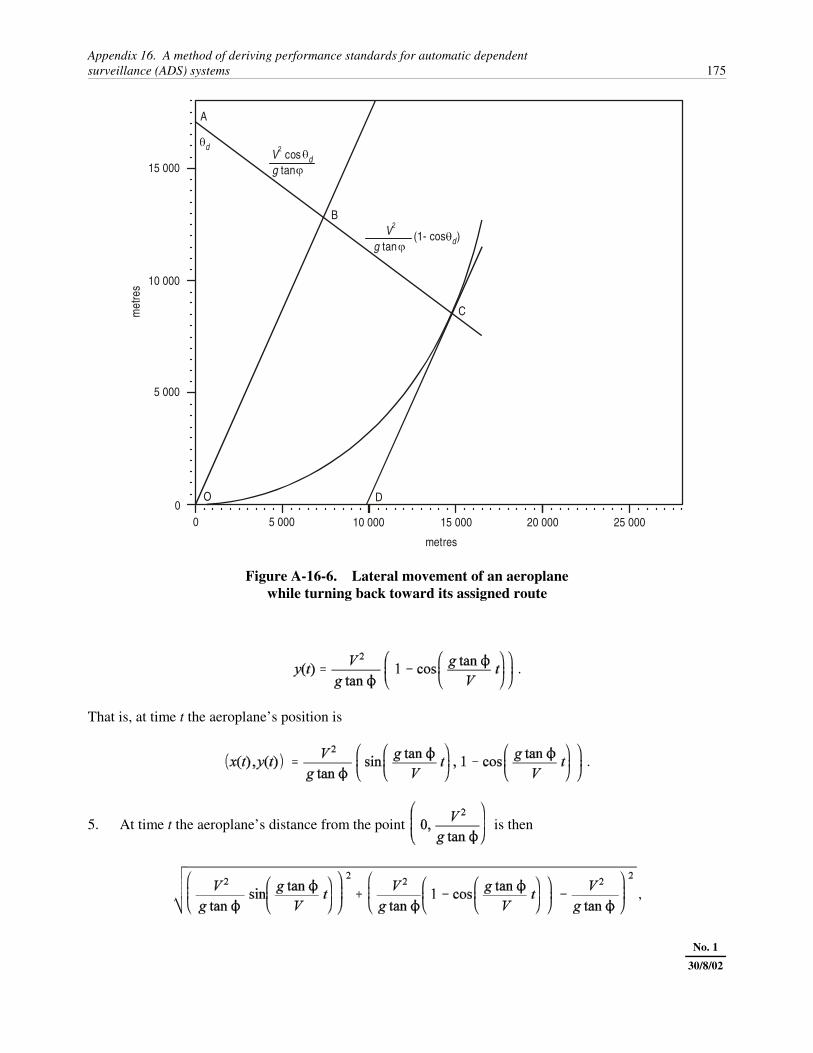
Appendix 16. A method of deriving performance standards for automatic dependentsurveillance (ADS) systems 175
No. 1
30/8/02
00
5 000 10 000 15 000 20 000 25 000
5 000
10 000
15 000
metres
met
res
A
C
B
DO
ddV2 cos
g tan
dg tanV2
(1- cos )
Figure A-16-6. Lateral movement of an aeroplanewhile turning back toward its assigned route
.
That is, at time t the aeroplane’s position is
.
5. At time t the aeroplane’s distance from the point is then
,

176 Manual on Airspace Planning Methodology for the Determination of Separation Minima
No. 1
30/8/02
which is easily simplified to . Since this distance is not a function of t, but is a constant, the aircraft’s
path during its turn must lie along the circle of radius about the point . In Figure A-16-6
the aeroplane’s path is shown as arc OC, and the circle’s centre, , is labelled point A.
6. When the aircraft begins its turn, it is headed along the X-axis, so that the angle between its velocity vectorand the X-axis is 0. As the turn progresses, the velocity vector rotates away from the X-axis. Since theaeroplane’s path lies along a circle, the central angle subtended by the path at time t, �(t), is also the angle by
which the velocity vector has rotated away from the X-axis. The tangent of that angle is , and the
expressions derived above for vx(t) and vy(t) immediately yield the result , from which
it follows (since the tangent function is one-to-one on ) that , or .
7. Let �d denote the angle at which the aeroplane deviates from its cleared route before beginning its turn.It needs to turn through the same angle before it can begin to head back toward the route. It reaches itsmaximum distance from the route at the instant when it has turned through that angle and is (momentarily)heading parallel to the route. In Figure A-16-6, that occurs when the aeroplane is at point C. The tangent to thecircle at C intersects the X-axis at a point D, so line segment is parallel to the cleared route. Line segment is drawn parallel to segment (and is therefore also parallel to the cleared route), and it passes through O= (0,0), the point at which the aeroplane began its turn.
8. Since is tangent to the circle at C, the radius is perpendicular to , and the cleared routeof flight, and so the length of segment is the distance that the aeroplane moved away from the cleared routebetween the time it began its turn and the time it started moving back toward the route. Triangle ABO is a right
triangle whose hypotenuse has length , and angle OAB has measure . Thus the length of segment
must be . Since the radius has length , the length of segment must be
.