00000chen- linear regression analysis3
TRANSCRIPT
8/13/2019 00000chen- Linear Regression Analysis3
http://slidepdf.com/reader/full/00000chen-linear-regression-analysis3 1/252
MultipleRegression Analysis
y = 0 + 1 x 1 + 2 x 2 + . . . p x p + ε
12013/11/27 Chia-Hsin Chen

8/13/2019 00000chen- Linear Regression Analysis3
http://slidepdf.com/reader/full/00000chen-linear-regression-analysis3 2/252
Assumptions of OLS
Estimator

8/13/2019 00000chen- Linear Regression Analysis3
http://slidepdf.com/reader/full/00000chen-linear-regression-analysis3 3/252
Regression Residual
A regression residual, , is defined as the
difference between an observed y value and its
corresponding predicted value:
0 1 1 2 2ˆ ˆ ˆ ˆˆ ˆ b b b b
k k y y y x x x
2013/11/27

8/13/2019 00000chen- Linear Regression Analysis3
http://slidepdf.com/reader/full/00000chen-linear-regression-analysis3 4/252
Assumptions of OLS Estimator
1) E(εi
) = 0 (unbiasedness)
2) Var(ε i) is constant (homoscedasticity)
3) Cov(ε i, ε j) = 0 (independent error terms)
4) Cov(ε i,Xi) = 0 (error terms unrelated to X’s) ε i ~ iid (0 , 2)
Gauss-Markov Theorem: If these conditions hold,
OLS is the best linear unbiased estimator (BLUE).Additional Assumption: ε i’s are normally distributed.
8/13/2019 00000chen- Linear Regression Analysis3
http://slidepdf.com/reader/full/00000chen-linear-regression-analysis3 5/252
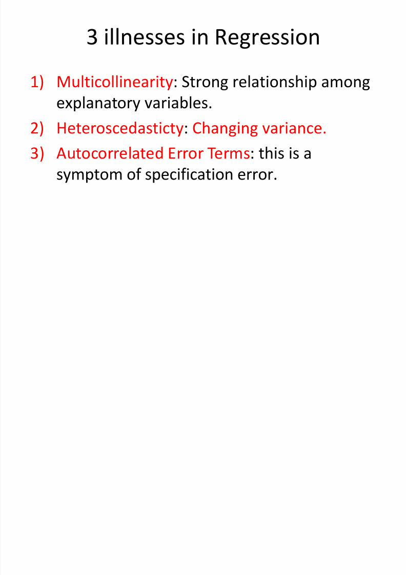
3 illnesses in Regression
1) Multicollinearity: Strong relationship among
explanatory variables.
2) Heteroscedasticty: Changing variance.
3) Autocorrelated Error Terms: this is a
symptom of specification error.
8/13/2019 00000chen- Linear Regression Analysis3
http://slidepdf.com/reader/full/00000chen-linear-regression-analysis3 6/252
Checking the Regression
Assumptions

8/13/2019 00000chen- Linear Regression Analysis3
http://slidepdf.com/reader/full/00000chen-linear-regression-analysis3 7/252
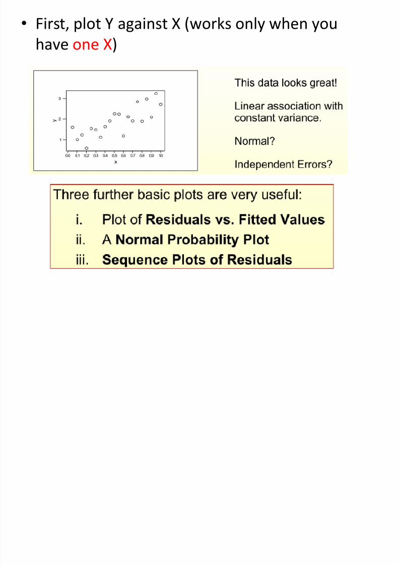
Assumptions of the model:
1) linear conditional mean
2) constant variance (homoskedasticity), normal errors
3) independent error terms
So we should see:
– a pattern of constant variation around a line
– very few points more than 2 standard deviations
away from central linear relationship.
How can we be sure of this when using real data? Wemust perform some basic diagnostic procedures to
insure that the model holds

8/13/2019 00000chen- Linear Regression Analysis3
http://slidepdf.com/reader/full/00000chen-linear-regression-analysis3 8/252
If the model assumptions are violated:
– Prediction can be systematically biased
– Standard errors and t-tests wrong
– someone may be able to beat you with adifferent and better model
All of the assumptions of the model are
really statements about the regression errorterms (ε).
How can we detect violations of the model?

8/13/2019 00000chen- Linear Regression Analysis3
http://slidepdf.com/reader/full/00000chen-linear-regression-analysis3 9/252
Example: Data Set 1

8/13/2019 00000chen- Linear Regression Analysis3
http://slidepdf.com/reader/full/00000chen-linear-regression-analysis3 10/252
Example: Data Set 2
8/13/2019 00000chen- Linear Regression Analysis3
http://slidepdf.com/reader/full/00000chen-linear-regression-analysis3 11/252
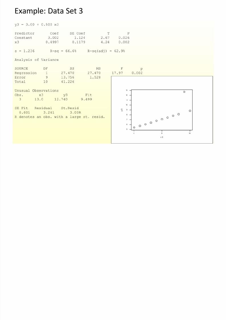
Example: Data Set 3

8/13/2019 00000chen- Linear Regression Analysis3
http://slidepdf.com/reader/full/00000chen-linear-regression-analysis3 12/252
Example: Data Set 4

8/13/2019 00000chen- Linear Regression Analysis3
http://slidepdf.com/reader/full/00000chen-linear-regression-analysis3 13/252
Residual Analysis

8/13/2019 00000chen- Linear Regression Analysis3
http://slidepdf.com/reader/full/00000chen-linear-regression-analysis3 14/252
Properties of
Regression Residual
The mean of the residuals is equal to 0.
• This property follows from the fact that the
sum of the differences between the observed
y values and their least squares predicted
values is equal to 0.
ˆResiduals 0 y y
ˆ y
2013/11/27
8/13/2019 00000chen- Linear Regression Analysis3
http://slidepdf.com/reader/full/00000chen-linear-regression-analysis3 15/252
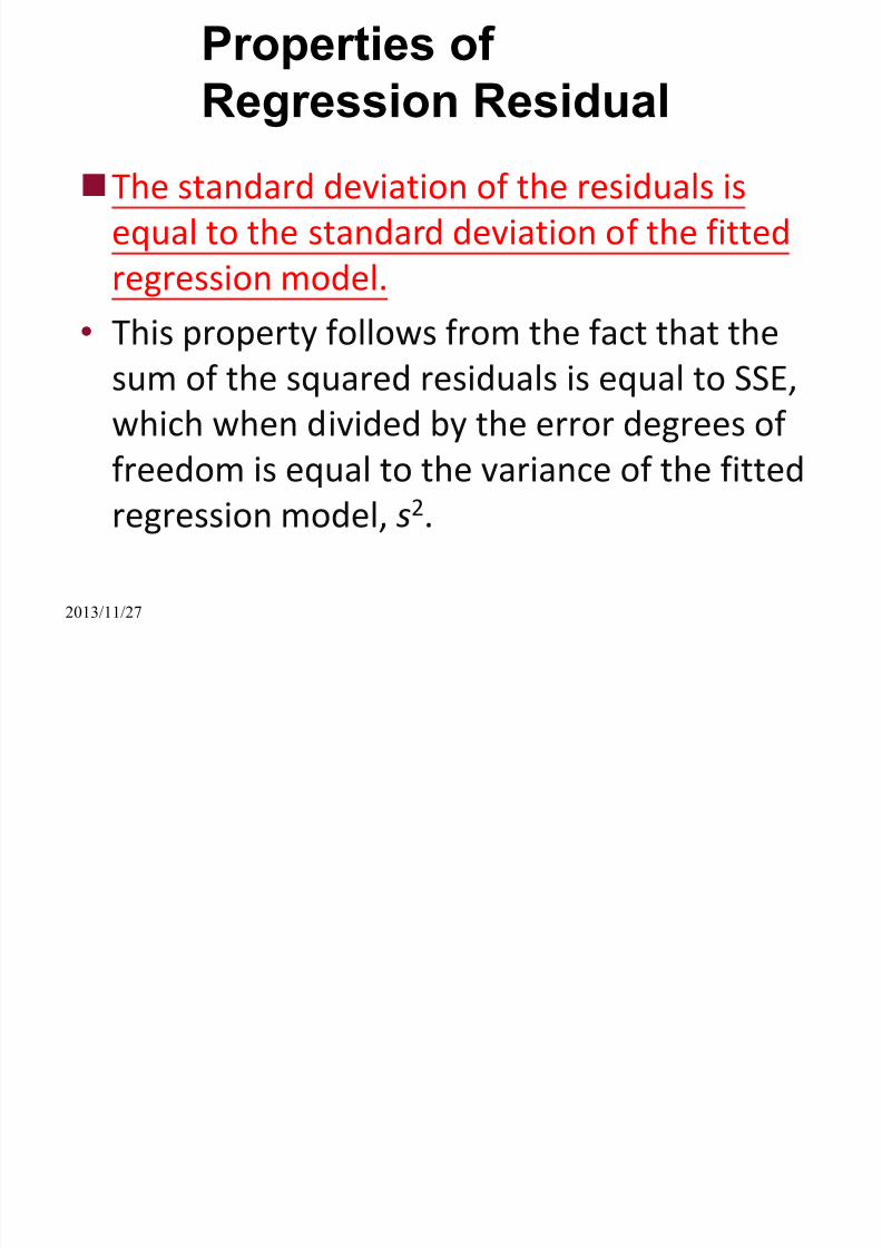
Properties of
Regression Residual
The standard deviation of the residuals is
equal to the standard deviation of the fitted
regression model.
• This property follows from the fact that the
sum of the squared residuals is equal to SSE,
which when divided by the error degrees of
freedom is equal to the variance of the fitted
regression model, s2.
2013/11/27

8/13/2019 00000chen- Linear Regression Analysis3
http://slidepdf.com/reader/full/00000chen-linear-regression-analysis3 16/252
Properties of
Regression Residual
The square root of the variance is both the
standard deviation of the residuals and the
standard deviation of the regression model.
2 2
2
ˆResiduals SSE
Residuals SSE
1 1
y y
sn k n k
2013/11/27

8/13/2019 00000chen- Linear Regression Analysis3
http://slidepdf.com/reader/full/00000chen-linear-regression-analysis3 17/252
Regression Outlier
A regression outlier is a residual that is larger
than 3s (in absolute value).
2013/11/27

8/13/2019 00000chen- Linear Regression Analysis3
http://slidepdf.com/reader/full/00000chen-linear-regression-analysis3 18/252
Heteroskedasticity

8/13/2019 00000chen- Linear Regression Analysis3
http://slidepdf.com/reader/full/00000chen-linear-regression-analysis3 19/252
• Heteroskedasticity : the error terms do not all
have the same variance.
8/13/2019 00000chen- Linear Regression Analysis3
http://slidepdf.com/reader/full/00000chen-linear-regression-analysis3 20/252

8/13/2019 00000chen- Linear Regression Analysis3
http://slidepdf.com/reader/full/00000chen-linear-regression-analysis3 21/252
Consequences of Using OLS
when Heteroscedasticity
OLS estimation still gives unbiased coefficient
estimates, but they are no longer BLUE.
• This implies that if we still use OLS in the
presence of heteroscedasticity, our standarderrors could be inappropriate and hence any
inferences we make could be misleading.
• Whether the standard errors calculated using theusual formulae are too big or too small will
depend upon the form of the heteroscedasticity.

8/13/2019 00000chen- Linear Regression Analysis3
http://slidepdf.com/reader/full/00000chen-linear-regression-analysis3 22/252
Detection of Heteroscedasticity
Graphical methods
Formal tests: There are many of them
• Goldfeld-Quandt (GQ) test• White’s test
• ……

8/13/2019 00000chen- Linear Regression Analysis3
http://slidepdf.com/reader/full/00000chen-linear-regression-analysis3 23/252
Graphical analysis of residuals
To check for homoscedasticity (constant variance):
— Produce a scatterplot of the standardized residualsagainst the fitted values.
— Produce a scatterplot of the standardized residuals
against each of the independent variables.
• If assumptions are satisfied, residuals should varyrandomly around zero and the spread of theresiduals should be about the same throughoutthe plot (no systematic patterns.)
2013/11/27
8/13/2019 00000chen- Linear Regression Analysis3
http://slidepdf.com/reader/full/00000chen-linear-regression-analysis3 24/252

8/13/2019 00000chen- Linear Regression Analysis3
http://slidepdf.com/reader/full/00000chen-linear-regression-analysis3 25/252
1.Plot of Residuals vs. Fitted Values
Useful for:
• detection of non-linear relationships
• detection of non-constant variances
What should this look like?
• 1. Residuals should be evenly distributed
around the mean
• 2. No relationship between the mean of the
residual and the level of fitted value

8/13/2019 00000chen- Linear Regression Analysis3
http://slidepdf.com/reader/full/00000chen-linear-regression-analysis3 26/252
A key assumption is that the
regression model is a linear
function. This is not always true.This will show up even more
prominently in the residuals vs.
fitted plot…
r e s i d u
a l s
There should be no
relationship between the
average value of the
residuals and fitted (X)
8/13/2019 00000chen- Linear Regression Analysis3
http://slidepdf.com/reader/full/00000chen-linear-regression-analysis3 27/252
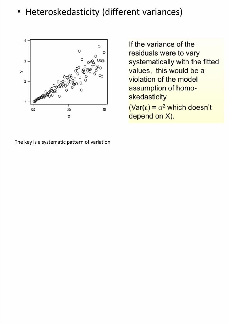
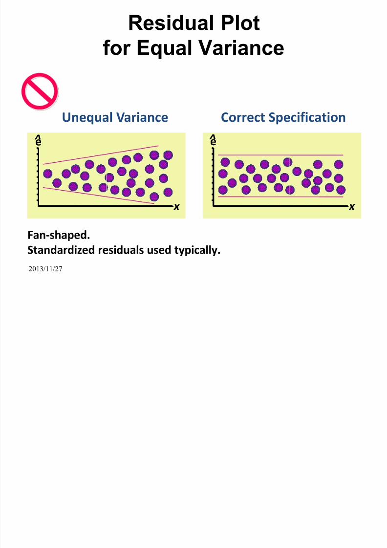
• Heteroskedasticity (different variances)
The key is a systematic pattern of variation
8/13/2019 00000chen- Linear Regression Analysis3
http://slidepdf.com/reader/full/00000chen-linear-regression-analysis3 28/252
r e s i d u a l s
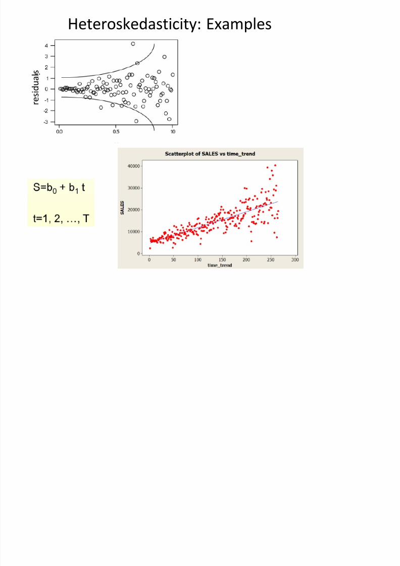
Heteroskedasticity: Examples

8/13/2019 00000chen- Linear Regression Analysis3
http://slidepdf.com/reader/full/00000chen-linear-regression-analysis3 29/252
Homoscedasticity is probably violated if…
The residuals seem to increase or decrease inaverage magnitude with the fitted values, it isan indication that the variance of the residuals
is not constant.
The points in the plot lie on a curve aroundzero, rather than fluctuating randomly.
A few points in the plot lie a long way fromthe rest of the points.

8/13/2019 00000chen- Linear Regression Analysis3
http://slidepdf.com/reader/full/00000chen-linear-regression-analysis3 30/252
Residual Plot
for Functional Form
Add x 2 Term Correct Specification
x
e ^
x
e ^
2013/11/27
0
8/13/2019 00000chen- Linear Regression Analysis3
http://slidepdf.com/reader/full/00000chen-linear-regression-analysis3 31/252
8/13/2019 00000chen- Linear Regression Analysis3
http://slidepdf.com/reader/full/00000chen-linear-regression-analysis3 32/252
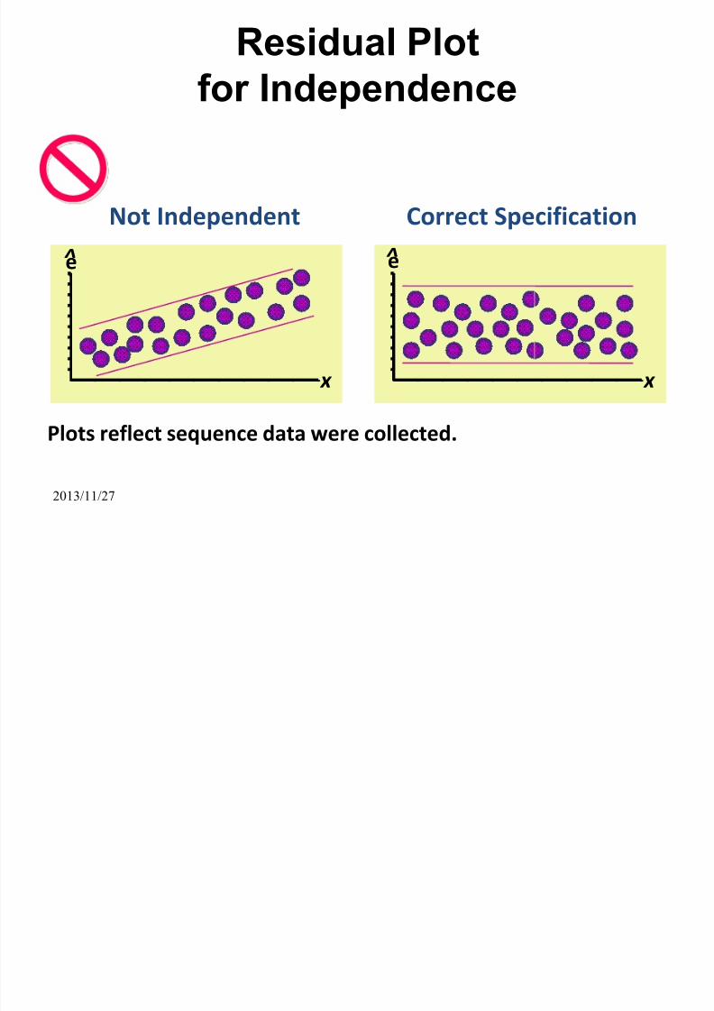
Residual Plot
for Independence
x
Not Independent Correct Specification
Plots reflect sequence data were collected.
e ^
x
e ^
2013/11/27

8/13/2019 00000chen- Linear Regression Analysis3
http://slidepdf.com/reader/full/00000chen-linear-regression-analysis3 33/252
Testing the Normality
Assumption
8/13/2019 00000chen- Linear Regression Analysis3
http://slidepdf.com/reader/full/00000chen-linear-regression-analysis3 34/252
Normality of residuals.
Normality is not required in order to obtain
unbiased estimates of the regression
coefficients.
• But normality of the residuals necessary forsome of the other tests – for example the
Bresch Pagan test of heteroscedasticity, Durbin
Watson test of autocorrelation, etc.

8/13/2019 00000chen- Linear Regression Analysis3
http://slidepdf.com/reader/full/00000chen-linear-regression-analysis3 35/252
Normality of residuals.
Non-normal residuals cause the following:• t-tests and other associated statistics may no
longer be t distributed
• Least squares estimates are extremely sensitiveto large εi and it may be possible to improve on
least squares
• The linear functional form may be incorrect andvarious transformations of the dependent
variable may be necessary.

8/13/2019 00000chen- Linear Regression Analysis3
http://slidepdf.com/reader/full/00000chen-linear-regression-analysis3 36/252
Normality
The random errors need be regarded as a random
sample from a N(0,σ2) distribution, so we can
check this assumption by checking whether the
residuals might have come from a normaldistribution.
We should look at the standardized residuals
Options for looking at distribution:
• Histogram,
• Normal plot of residuals

8/13/2019 00000chen- Linear Regression Analysis3
http://slidepdf.com/reader/full/00000chen-linear-regression-analysis3 37/252
How can we detect departures from normality?
• Characteristics of the normal distribution : thin tails
and symmetry.• The most basic analysis would be to graph the
histogram of the standardized residuals.
Neither of these plots look particularly symmetric
Histogram

8/13/2019 00000chen- Linear Regression Analysis3
http://slidepdf.com/reader/full/00000chen-linear-regression-analysis3 38/252
ExampleHistogram with a normal curve for recent 61 observations
of the monthly stock rate of return of Exxon
The histogram uses only 61
observations, whereas the normal
curve superimposed depicts the
histogram using infinitely many
observations. Therefore, sampling
errors should show up as gaps
between the two curves.
This is not effective for revealing a subtle but systematic
departure of the histogram from normality.

8/13/2019 00000chen- Linear Regression Analysis3
http://slidepdf.com/reader/full/00000chen-linear-regression-analysis3 39/252
Normal Q-Q Plot of Residuals
A normal probability plot is found by plotting the residualsof the observed sample against the corresponding residualsof a standard normal distribution N (0,1)
1) The first step is to sort the data from the lowest to thehighest. Let n be the number of observations. Then, the
lowest observation, denoted as x(1) is the (1/n) th quantileof the data.
2) The next step is to determine for each observation thecorresponding quantile of the normal distribution that hasthe same mean and the standard deviation as the data. The
following Excel function is a convenient way to determinethe normal (i/(n+1)) th quantile, denoted as x’(i).
x’(i) = NORMINV(i/(n+1), sample mean, sample standard deviation).
N l Q Q l t

8/13/2019 00000chen- Linear Regression Analysis3
http://slidepdf.com/reader/full/00000chen-linear-regression-analysis3 40/252
• If the plot shows a straight line, it is
reasonable to assume that the observedsample comes from a normal distribution.
• If the points deviate a lot from a straight line,
there is evidence against the assumption thatthe random errors are an independent samplefrom a normal distribution.
x’(i)
i/(n+1)
Normal Q-Q plot

8/13/2019 00000chen- Linear Regression Analysis3
http://slidepdf.com/reader/full/00000chen-linear-regression-analysis3 41/252
Normal Q-Q Plot
• qq-plots plot the quantiles of a variable
against the quantiles of a normal
distribution.
• qq plot is sensitive to non-normality
near the tails.

8/13/2019 00000chen- Linear Regression Analysis3
http://slidepdf.com/reader/full/00000chen-linear-regression-analysis3 42/252
1) The data are arranged from smallest to largest.2) The percentile of each data value is determined.
3) the z-score of each data value is calculated.
4) z-scores are plotted against the percentiles ofdata values
Departures from this straight line indicatedepartures from normality.
PP-plot is sensitive to non-normality in the middlerange of data.
PP-plot graphs
PP-plot graphs

8/13/2019 00000chen- Linear Regression Analysis3
http://slidepdf.com/reader/full/00000chen-linear-regression-analysis3 43/252
PP-plot graphs
8/13/2019 00000chen- Linear Regression Analysis3
http://slidepdf.com/reader/full/00000chen-linear-regression-analysis3 44/252
Example
l

8/13/2019 00000chen- Linear Regression Analysis3
http://slidepdf.com/reader/full/00000chen-linear-regression-analysis3 45/252
Example
Suppose simulate some data from a t distribution with only 3
degrees of freedom.
8/13/2019 00000chen- Linear Regression Analysis3
http://slidepdf.com/reader/full/00000chen-linear-regression-analysis3 46/252
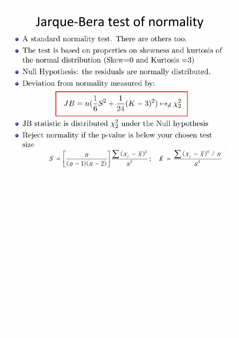
Jarque-Bera test of normality
3 4
3 4
( ) ( ) /;
( 1)( 2)
i i x x x x n n
S K
n n s s
k

8/13/2019 00000chen- Linear Regression Analysis3
http://slidepdf.com/reader/full/00000chen-linear-regression-analysis3 47/252
眾 數 平均 數中 位 數 x
f ( x )
眾 數平 均 數 x中 位 數
( x )
中 位
數
=平
均
數
=眾
數
( x )
x
skewness
Skewed to the right, SK>0
Skewed to the left, SK<0
3
3( )
( 1)( 2)
i x x n S n n s

8/13/2019 00000chen- Linear Regression Analysis3
http://slidepdf.com/reader/full/00000chen-linear-regression-analysis3 48/252
kurtosis
( X )
高窄峰
低闊峰
常態峰
4
4
( ) /i
x x n K
s
What can we do if we find evidence of

8/13/2019 00000chen- Linear Regression Analysis3
http://slidepdf.com/reader/full/00000chen-linear-regression-analysis3 49/252
What can we do if we find evidence ofNon-Normality?
What is the pattern in the plot of residuals?Check alternative (non-linear) specifications that
are appropriate.
Deviations from normality could be due tooutliers.
– Find the reasons for outliers.
– Data error? Correct the entry. – If not data error, and there is a valid reason for that
observation, then could use a dummy variable for
that observation.
8/13/2019 00000chen- Linear Regression Analysis3
http://slidepdf.com/reader/full/00000chen-linear-regression-analysis3 50/252
8/13/2019 00000chen- Linear Regression Analysis3
http://slidepdf.com/reader/full/00000chen-linear-regression-analysis3 51/252
What should you do about outliers?
Investigate – data errors, changes in
measurement,
structural changes in the environment
Consider deleting only if you have a good reason.
What is an outlier?
– an unusual observation which is not likely to reoccur.
– If it is likely to reoccur, you will fool yourself bydeletion. You will think that the model fits and
predicts better than it really does.

8/13/2019 00000chen- Linear Regression Analysis3
http://slidepdf.com/reader/full/00000chen-linear-regression-analysis3 52/252
St i

8/13/2019 00000chen- Linear Regression Analysis3
http://slidepdf.com/reader/full/00000chen-linear-regression-analysis3 53/252
Steps in a
Residual Analysis
1. Check for a misspecified model by plotting
the residuals against each of the quantitative
independent variables.
• Analyze each plot, looking for a curvilinear
trend. This shape signals the need for a
quadratic term in the model. Try a second-
order term in the variable against which theresiduals are plotted.
2013/11/27
St i R id l A l i

8/13/2019 00000chen- Linear Regression Analysis3
http://slidepdf.com/reader/full/00000chen-linear-regression-analysis3 54/252
Steps in a Residual Analysis
2. Examine the residual plots for outliers. Draw
lines on the residual plots at 2- and 3-standard-deviation distances below andabove the 0 line.
• Examine residuals outside the 3-standard-deviation lines as potential outliers and checkto see that no more than 5% of the residualsexceed the 2-standard-deviation lines.
2013/11/27

8/13/2019 00000chen- Linear Regression Analysis3
http://slidepdf.com/reader/full/00000chen-linear-regression-analysis3 55/252
St i
8/13/2019 00000chen- Linear Regression Analysis3
http://slidepdf.com/reader/full/00000chen-linear-regression-analysis3 56/252
Steps in a
Residual Analysis
3. Check for nonnormal errors by plotting afrequency distribution of the residuals, usinga stem-and-leaf display or a histogram.
• Check to see if obvious departures fromnormality exist. Extreme skewness of thefrequency distribution may be due to outliers
or could indicate the need for atransformation of the dependent variable.
2013/11/27
Steps in a

8/13/2019 00000chen- Linear Regression Analysis3
http://slidepdf.com/reader/full/00000chen-linear-regression-analysis3 57/252
Steps in a
Residual Analysis
4. Check for unequal error variances by plottingthe residuals against the predicted values, .If you detect a cone-shaped pattern or some
other pattern that indicates that the varianceof is not constant, refit the model using anappropriate variance-stabilizing transformation on y , such as ln (y ). (Consultthe references for other useful variance-stabilizing transformations.)
2013/11/27

8/13/2019 00000chen- Linear Regression Analysis3
http://slidepdf.com/reader/full/00000chen-linear-regression-analysis3 58/252
Goldfeld-Quandt (GQ) test
The Goldfeld-Quandt (GQ) test is carried outas follows.
1) Split the total sample of length T into two
sub-samples of length T1 and T2. Theregression model is estimated on each sub-sample and the two residual variances arecalculated.
2) The null hypothesis is that the variances ofthe disturbances are equal, H0: 2
2
2
1

8/13/2019 00000chen- Linear Regression Analysis3
http://slidepdf.com/reader/full/00000chen-linear-regression-analysis3 59/252

8/13/2019 00000chen- Linear Regression Analysis3
http://slidepdf.com/reader/full/00000chen-linear-regression-analysis3 60/252
• White’s general test for heteroscedasticity is oneof the best approaches because it makes fewassumptions about the form of theheteroscedasticity.
• The test is carried out as follows:1) Assume that the regression we carried out is as
follows y t = 1 + 2x 2t + 3x 3t + u t
And we want to test H0: Var(u t ) = 2
.We estimate the model, obtaining the residuals .
White’s Test: Detection of Heteroscedasticity
ut

8/13/2019 00000chen- Linear Regression Analysis3
http://slidepdf.com/reader/full/00000chen-linear-regression-analysis3 61/252
2) Then run the auxiliary regression
3) Obtain R2 from the auxiliary regression and multiply it
by the number T of observations. It can be shown thatT R2 2 (m)
where m is the number of regressors in the auxiliaryregression excluding the constant term.
4) If the 2
test statistic from step 3 is greater than thecorresponding value from the statistical table, then rejectthe null hypothesis that the disturbances arehomoscedastic.
t t t t t t t t v x x x x x xu 326
2
35
2
2433221
2ˆ

8/13/2019 00000chen- Linear Regression Analysis3
http://slidepdf.com/reader/full/00000chen-linear-regression-analysis3 62/252
How Do we Deal with
Heteroscedasticity?
8/13/2019 00000chen- Linear Regression Analysis3
http://slidepdf.com/reader/full/00000chen-linear-regression-analysis3 63/252
Generalised Least Squares (GLS)
If the form (i.e. the cause) of the heteroscedasticity is
known, then we can use an estimation method
which takes this into account (called generalised
least squares, GLS).
G li d L t S (GLS)

8/13/2019 00000chen- Linear Regression Analysis3
http://slidepdf.com/reader/full/00000chen-linear-regression-analysis3 64/252
Generalised Least Squares (GLS)
A simple illustration of GLS is as follows: Suppose
that the error variance is related to another variable
zt by
• To remove the heteroscedasticity, divide the
regression equation by zt. Than
where is the error term.
So the disturbances from the new regression
equation will be homoscedastic.
22var t t z u
t
t
t
t
t
t t
t v z
x
z
x
z z
y 3
32
21
1 b b b
t
t t
z
uv
2
2
22
2
var var var
t
t
t
t
t
t t
z
z
z
u
z
uv

8/13/2019 00000chen- Linear Regression Analysis3
http://slidepdf.com/reader/full/00000chen-linear-regression-analysis3 65/252
Other Correcting for Heteroskedasticity

8/13/2019 00000chen- Linear Regression Analysis3
http://slidepdf.com/reader/full/00000chen-linear-regression-analysis3 66/252
Other Correcting for Heteroskedasticity
Use White’s heteroscedasticity consistentstandard error estimates.
• The effect of using White’s correction is that in
general the standard errors for the slopecoefficients are increased relative to the usualOLS standard errors.
• This makes us more “conservative” in hypothesis
testing, so that we would need more evidenceagainst the null hypothesis before we wouldreject it.
E l

8/13/2019 00000chen- Linear Regression Analysis3
http://slidepdf.com/reader/full/00000chen-linear-regression-analysis3 67/252
Example
8/13/2019 00000chen- Linear Regression Analysis3
http://slidepdf.com/reader/full/00000chen-linear-regression-analysis3 68/252

8/13/2019 00000chen- Linear Regression Analysis3
http://slidepdf.com/reader/full/00000chen-linear-regression-analysis3 69/252
8/13/2019 00000chen- Linear Regression Analysis3
http://slidepdf.com/reader/full/00000chen-linear-regression-analysis3 70/252
8/13/2019 00000chen- Linear Regression Analysis3
http://slidepdf.com/reader/full/00000chen-linear-regression-analysis3 71/252

8/13/2019 00000chen- Linear Regression Analysis3
http://slidepdf.com/reader/full/00000chen-linear-regression-analysis3 72/252

8/13/2019 00000chen- Linear Regression Analysis3
http://slidepdf.com/reader/full/00000chen-linear-regression-analysis3 73/252

8/13/2019 00000chen- Linear Regression Analysis3
http://slidepdf.com/reader/full/00000chen-linear-regression-analysis3 74/252
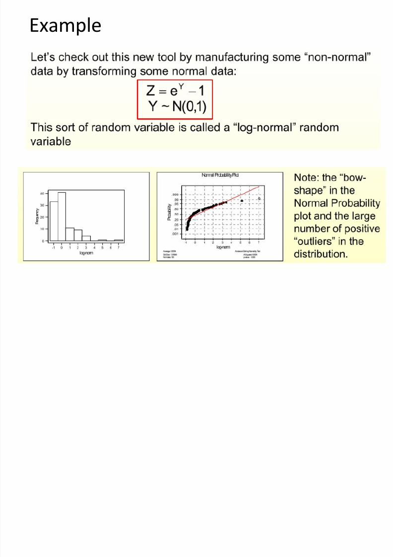
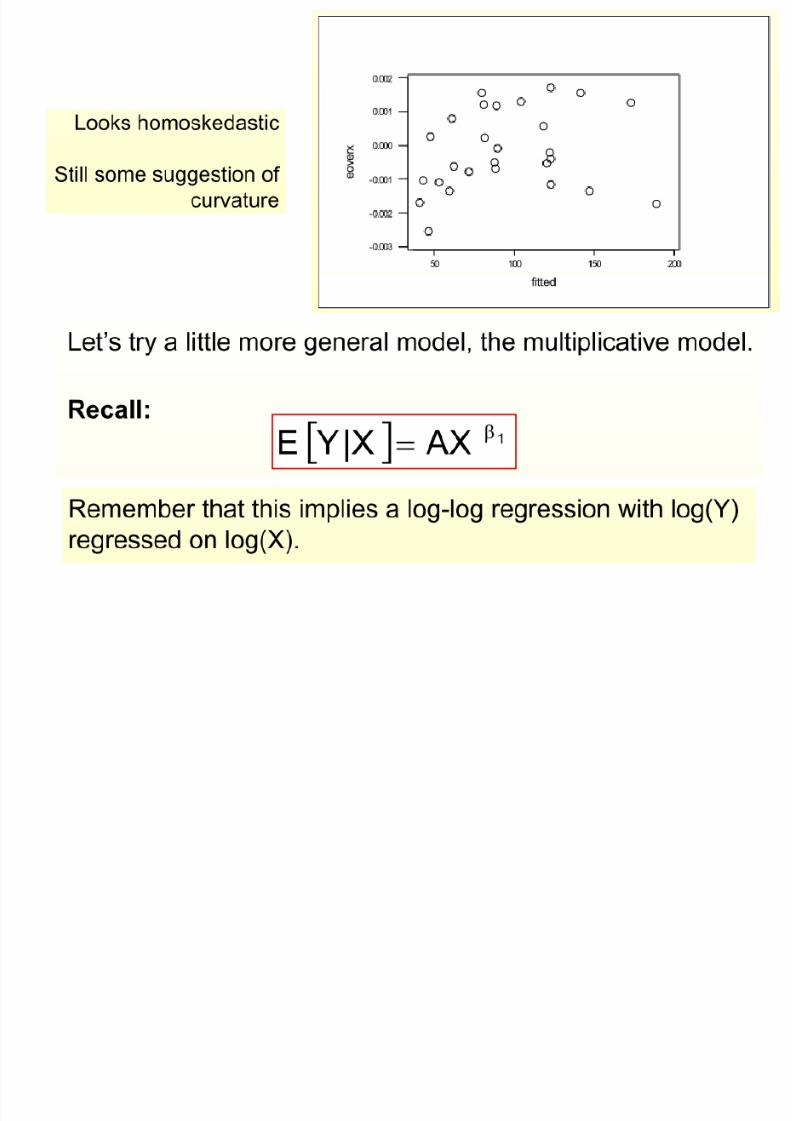
Reasons for the Log Transform

8/13/2019 00000chen- Linear Regression Analysis3
http://slidepdf.com/reader/full/00000chen-linear-regression-analysis3 75/252

8/13/2019 00000chen- Linear Regression Analysis3
http://slidepdf.com/reader/full/00000chen-linear-regression-analysis3 76/252
1
Y X
Y b

8/13/2019 00000chen- Linear Regression Analysis3
http://slidepdf.com/reader/full/00000chen-linear-regression-analysis3 77/252

8/13/2019 00000chen- Linear Regression Analysis3
http://slidepdf.com/reader/full/00000chen-linear-regression-analysis3 78/252

8/13/2019 00000chen- Linear Regression Analysis3
http://slidepdf.com/reader/full/00000chen-linear-regression-analysis3 79/252
Multicolinear
Multicollinearity

8/13/2019 00000chen- Linear Regression Analysis3
http://slidepdf.com/reader/full/00000chen-linear-regression-analysis3 80/252
Multicollinearity
This problem occurs when the explanatory variables are very
highly correlated with each other. Perfect multicollinearity
• Cannot estimate all the coefficients
e.g. suppose x3 = 2 x2
and the model is yt = b 1 + b 2 x2t + b 3 x3t + b 4 x4t + ut Problems if Near Multicollinearity is Present but Ignored
• R2 will be high but the individual coefficients will have highstandard errors.
• The regression becomes very sensitive to small changes in thespecification.
• Thus confidence intervals for the parameters will be very wide,and significance tests might therefore give inappropriateconclusions.
8/13/2019 00000chen- Linear Regression Analysis3
http://slidepdf.com/reader/full/00000chen-linear-regression-analysis3 81/252
8/13/2019 00000chen- Linear Regression Analysis3
http://slidepdf.com/reader/full/00000chen-linear-regression-analysis3 82/252

8/13/2019 00000chen- Linear Regression Analysis3
http://slidepdf.com/reader/full/00000chen-linear-regression-analysis3 83/252

8/13/2019 00000chen- Linear Regression Analysis3
http://slidepdf.com/reader/full/00000chen-linear-regression-analysis3 84/252
8/13/2019 00000chen- Linear Regression Analysis3
http://slidepdf.com/reader/full/00000chen-linear-regression-analysis3 85/252

8/13/2019 00000chen- Linear Regression Analysis3
http://slidepdf.com/reader/full/00000chen-linear-regression-analysis3 86/252
8/13/2019 00000chen- Linear Regression Analysis3
http://slidepdf.com/reader/full/00000chen-linear-regression-analysis3 87/252
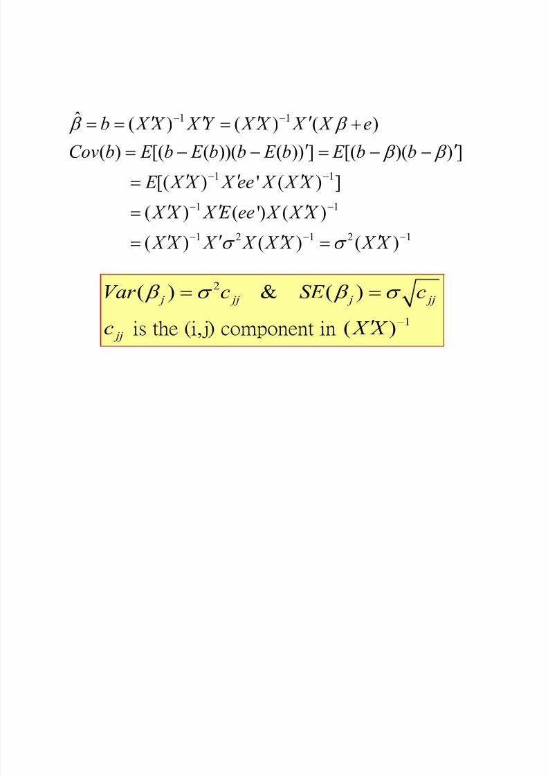
1 1
1 1
1 1
1 2 1 2 1
ˆ ( ) ( ) ( )
( ) [( ( ))( ( )) ] [( )( ) ]
[( ) ' ( ) ]
( ) ( ') ( )
( ) ( ) ( )
b b
b b
b X X X Y X X X X e
Cov b E b E b b E b E b b
E X X X ee X X X
X X X E ee X X X
X X X X X X X X
2
1
ˆ ˆ( ) & ( )
( )
b b
is the (i,j) component in
j jj j jj
jj
Var c SE c
c X X

8/13/2019 00000chen- Linear Regression Analysis3
http://slidepdf.com/reader/full/00000chen-linear-regression-analysis3 88/252

8/13/2019 00000chen- Linear Regression Analysis3
http://slidepdf.com/reader/full/00000chen-linear-regression-analysis3 89/252

8/13/2019 00000chen- Linear Regression Analysis3
http://slidepdf.com/reader/full/00000chen-linear-regression-analysis3 90/252
2 2
2 2
2 1
ˆ ˆ ˆ ˆ( ) ( )
ˆ ˆ( )
ˆ ˆ ˆ ˆ[ ( )][ ( )] [( )( ) ]
ˆ( ) ( )
Var Y E Y E Y E Y X
E X X E X
E X X XE X
XCov X X X X X
b
b b b b
b b b b b b b b
b
1ˆ( ) ( )SE Y X X X X
2 1ˆ( ) ( )Cov X X b
2
2 21
1
n
i
i
e
n k
M lti lli it
8/13/2019 00000chen- Linear Regression Analysis3
http://slidepdf.com/reader/full/00000chen-linear-regression-analysis3 91/252
Multicollinearity
• In multiple regression analysis, one is oftenconcerned with the nature and significance of the
relations between the explanatory variables and the
response variable.
• Questions that are frequently asked are:
– What is the relative importance of the effects of the
different independent variables?
– What is the magnitude of the effect of a given independentvariable on the dependent variable?
M lti lli it

8/13/2019 00000chen- Linear Regression Analysis3
http://slidepdf.com/reader/full/00000chen-linear-regression-analysis3 92/252
Multicollinearity
(A) Can any independent variable be dropped from themodel because it has little or no effect on the dependentvariable?
(B) Should any independent variables not yet includedin the model be considered for possible inclusion?
Simple answers can be given to these questions if
(A) The independent variables in the model areuncorrelated among themselves.
(B) They are uncorrelated with any other independentvariables that are related to the dependent variable butomitted from the model.

8/13/2019 00000chen- Linear Regression Analysis3
http://slidepdf.com/reader/full/00000chen-linear-regression-analysis3 93/252
M lti lli it

8/13/2019 00000chen- Linear Regression Analysis3
http://slidepdf.com/reader/full/00000chen-linear-regression-analysis3 94/252
Multicollinearity• Some key problems that typically arise when the
explanatory variables being considered for theregression model are highly correlated amongthemselves are:
1. Adding or deleting an explanatory variable changes the
regression coefficients.
2. The estimated standard deviations of the regressioncoefficients become large when the explanatoryvariables in the regression model are highly
correlated with each other.3. The estimated regression coefficients individually may
not be statistically significant even though a definitestatistical relation exists between the responsevariable and the set of explanatory variables.
Why?
Why?
Problems with multicolinearity

8/13/2019 00000chen- Linear Regression Analysis3
http://slidepdf.com/reader/full/00000chen-linear-regression-analysis3 95/252
Problems with multicolinearity
colinear variables can have coefficients with largestandard errors.
colinear variables can have insignificant t’s, but
very significant F’s
• getting a larger sample doesn’t necessarily help
much
• multicolinearity is a “disease”, a violation of the
model assumptions.• Least squares and the least squares standard errors
are not OK.
Multicollinearity
8/13/2019 00000chen- Linear Regression Analysis3
http://slidepdf.com/reader/full/00000chen-linear-regression-analysis3 96/252
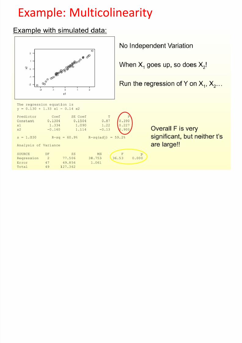
y(strong relationship among explanatory variables themselves)
Variances of regression coefficients are inflated (smaller).
Regression coefficients may be different from their true
values, even signs.
Adding or removing variables produces large changes in
coefficients.
Removing a data point may cause large changes in coefficient
estimates or signs.
In some cases, the F ratio may be significant, R 2 may be
very high despite the all t ratios are insignificant(suggesting no significant relationship).
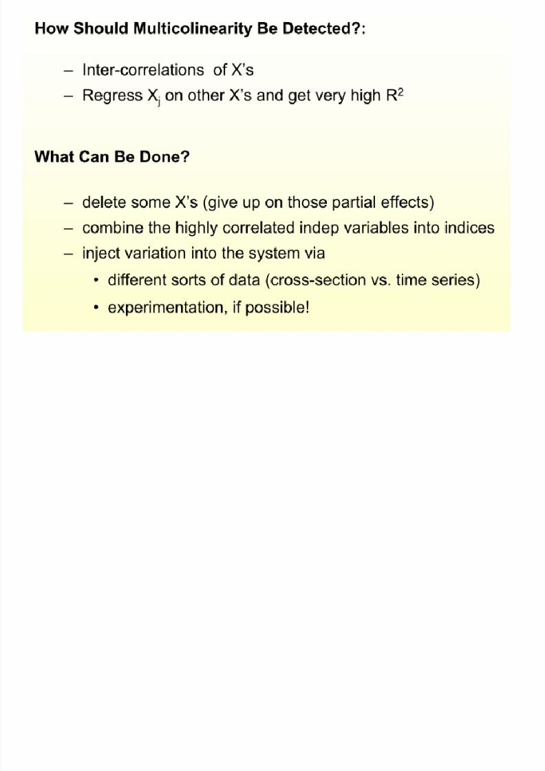
Solutions to the Multicollinearity Problem
8/13/2019 00000chen- Linear Regression Analysis3
http://slidepdf.com/reader/full/00000chen-linear-regression-analysis3 97/252
Solutions to the Multicollinearity Problem
Drop a collinear variable from theregression
Combine collinear variables (e.g. use their
sum as one variable)
Measuring Multicollinearity

8/13/2019 00000chen- Linear Regression Analysis3
http://slidepdf.com/reader/full/00000chen-linear-regression-analysis3 98/252
Measuring Multicollinearity
• The easiest way to measure the extent of multicollinearity
is simply to look at the matrix of correlations between theindividual variables. e.g.
• But another problem: if 3 or more variables are linear
- e.g. x2t + x3t = x4t
• Note that high correlation between y and one of the x’s isnot muticollinearity.
Corr x2 x3 x4
x2 - 0.2 0.8
x3 0.2 - 0.3
x4 0.8 0.3 -
Multicollinearity Diagnostics
8/13/2019 00000chen- Linear Regression Analysis3
http://slidepdf.com/reader/full/00000chen-linear-regression-analysis3 99/252
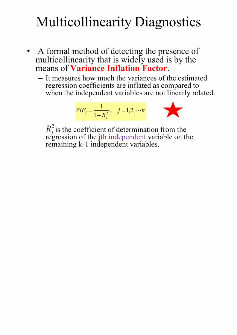
Multicollinearity Diagnostics
• A formal method of detecting the presence ofmulticollinearity that is widely used is by themeans of Variance Inflation Factor. – It measures how much the variances of the estimated
regression coefficients are inflated as compared towhen the independent variables are not linearly related.
– is the coefficient of determination from theregression of the jth independent variable on theremaining k-1 independent variables.
k j R
VIF j
j ,2,1,1
12
2 j R
Multicollinearity Diagnostics
8/13/2019 00000chen- Linear Regression Analysis3
http://slidepdf.com/reader/full/00000chen-linear-regression-analysis3 100/252
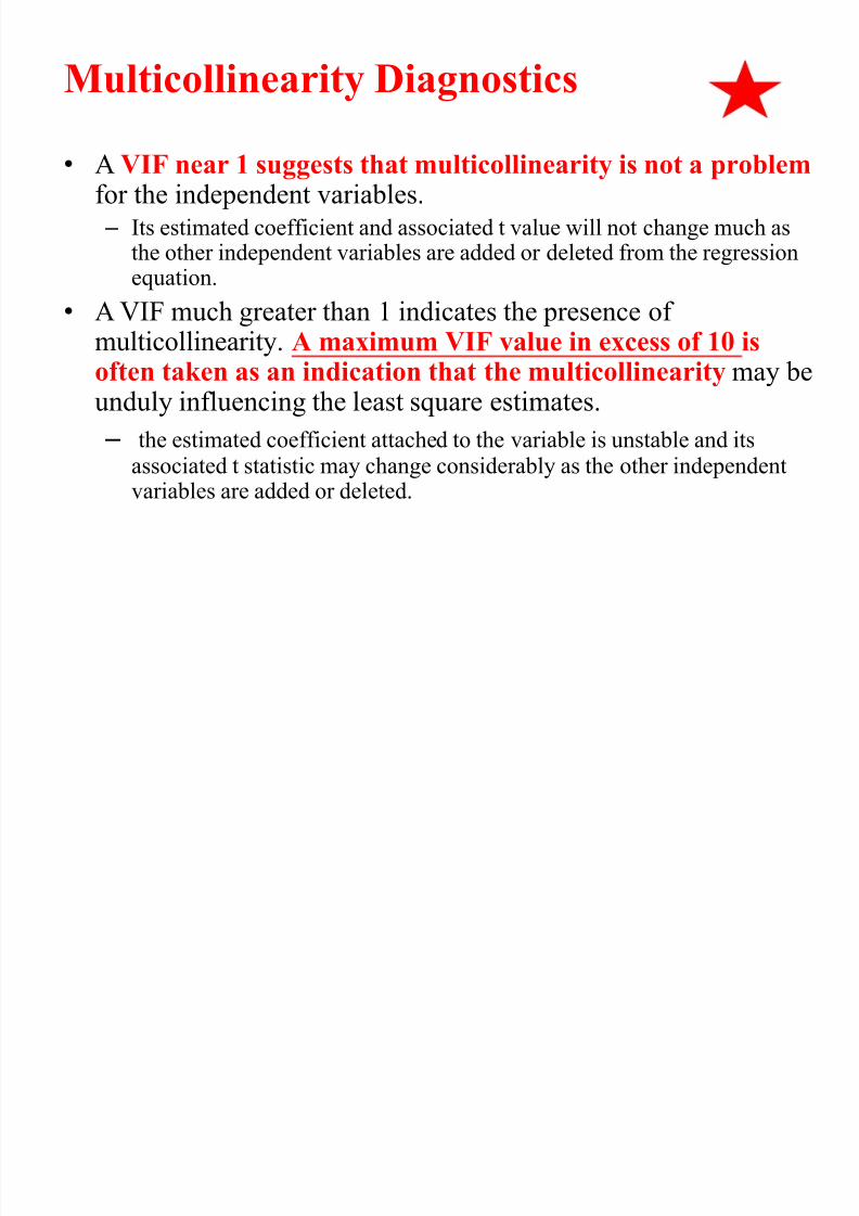
Multicollinearity Diagnostics
• A VIF near 1 suggests that multicollinearity is not a problemfor the independent variables. – Its estimated coefficient and associated t value will not change much as
the other independent variables are added or deleted from the regressionequation.
• A VIF much greater than 1 indicates the presence ofmulticollinearity. A maximum VIF value in excess of 10 isoften taken as an indication that the multicollinearity may beunduly influencing the least square estimates.
– the estimated coefficient attached to the variable is unstable and itsassociated t statistic may change considerably as the other independentvariables are added or deleted.
Multicollinearity Diagnostics

8/13/2019 00000chen- Linear Regression Analysis3
http://slidepdf.com/reader/full/00000chen-linear-regression-analysis3 101/252
Multicollinearity Diagnostics
• The simple correlation coefficient between all pairs ofexplanatory variables (i.e., X1, X2, …, Xk ) is helpfulin selecting appropriate explanatory variables for aregression model and is also critical for examining
multicollinearity.• While it is true that a correlation very close to +1
or – 1 does suggest multicollinearity, it is not true(unless there are only two explanatory variables)
to infer multicollinearity does not exist when thereare no high correlations between any pair ofexplanatory variables.
Example:Sales Forecasting
8/13/2019 00000chen- Linear Regression Analysis3
http://slidepdf.com/reader/full/00000chen-linear-regression-analysis3 102/252
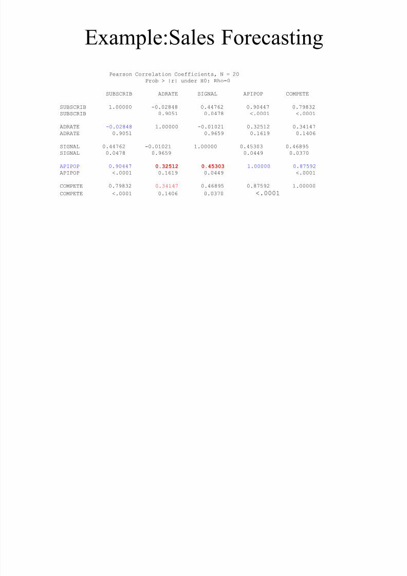
Example:Sales Forecasting
Pearson Correlation Coefficients, N = 20
Prob > |r| under H0: Rho=0
SUBSCRIB ADRATE SIGNAL APIPOP COMPETE
SUBSCRIB 1.00000 -0.02848 0.44762 0.90447 0.79832
SUBSCRIB 0.9051 0.0478 <.0001 <.0001
ADRATE -0.02848 1.00000 -0.01021 0.32512 0.34147
ADRATE 0.9051 0.9659 0.1619 0.1406
SIGNAL 0.44762 -0.01021 1.00000 0.45303 0.46895SIGNAL 0.0478 0.9659 0.0449 0.0370
APIPOP 0.90447 0.32512 0.45303 1.00000 0.87592
APIPOP <.0001 0.1619 0.0449 <.0001
COMPETE 0.79832 0.34147 0.46895 0.87592 1.00000
COMPETE <.0001 0.1406 0.0370 <.0001

8/13/2019 00000chen- Linear Regression Analysis3
http://slidepdf.com/reader/full/00000chen-linear-regression-analysis3 103/252
Example:Sales Forecasting
APIPOP495.0ADRATE25.028.96SUBSCRIBE
COMPETE16.23APIPOP44.0SIGNAL.02-ADRATE27.042.51SUBSCRIBE
COMPETE13.92APIPOP43.0ADRATE26.032.51SUBSCRIBE
Example:Sales Forecasting

8/13/2019 00000chen- Linear Regression Analysis3
http://slidepdf.com/reader/full/00000chen-linear-regression-analysis3 104/252
Example:Sales Forecasting
• VIF calculation: – Fit the model
COMPETE 3210 ADRATESIGNALAPIPOP b b b b
SUMMARY OUTPUT
Regression Statistics
Multiple R 0.878054
R Square 0.770978
Adjusted R Square 0.728036
Standard Error 264.3027
Observations 20
ANOVA
df SS MS F Significance F
Regression 3 3762601 1254200 17.9541 2.25472E-05
Residual 16 1117695 69855.92
Total 19 4880295
Coefficient andard Err t Stat P-value Lower 95% Upper 95%
Intercept -472.685 139.7492 -3.38238 0.003799 -768.9402258 -176.43
Compete 159.8413 28.29157 5.649786 3.62E-05 99.86587622 219.8168
ADRATE 0.048173 0.149395 0.322455 0.751283 -0.268529713 0.364876
Signal 0.037937 0.083011 0.457012 0.653806 -0.138038952 0.213913
Example:Sales Forecasting

8/13/2019 00000chen- Linear Regression Analysis3
http://slidepdf.com/reader/full/00000chen-linear-regression-analysis3 105/252
Example:Sales Forecasting
• Fit the model
SIGNAL 3210 APIPOPADRATECompete b b b b
SUMMARY OUTPUT
Regression Statistics
Multiple R 0.882936
R Square 0.779575
Adjusted R Square 0.738246
Standard Error 1.34954
Observations 20
ANOVA
df SS MS F Significance F
Regression 3 103.0599 34.35329 18.86239 1.66815E-05
Residual 16 29.14013 1.821258
Total 19 132.2
Coefficient andard Err t Stat P-value Lower 95% Upper 95%
Intercept 3.10416 0.520589 5.96278 1.99E-05 2.000559786 4.20776
ADRATE 0.000491 0.000755 0.649331 0.525337 -0.001110874 0.002092
Signal 0.000334 0.000418 0.799258 0.435846 -0.000552489 0.001221
APIPOP 0.004167 0.000738 5.649786 3.62E-05 0.002603667 0.005731
Example:Sales Forecasting

8/13/2019 00000chen- Linear Regression Analysis3
http://slidepdf.com/reader/full/00000chen-linear-regression-analysis3 106/252
Example:Sales Forecasting
• Fit the modelCOMPETE 3210 APIPOPADRATESignal b b b b
SUMMARY OUTPUT
Regression Statistics
Multiple R 0.512244
R Square 0.262394
Adjusted R Square 0.124092
Standard Error 790.8387
Observations 20
ANOVA
df SS MS F Significance F
Regression 3 3559789 1186596 1.897261 0.170774675
Residual 16 10006813 625425.8
Total 19 13566602
Coefficient andard Err t Stat P-value Lower 95% Upper 95%
Intercept 5.171093 547.6089 0.009443 0.992582 -1155.707711 1166.05
APIPOP 0.339655 0.743207 0.457012 0.653806 -1.235874129 1.915184
Compete 114.8227 143.6617 0.799258 0.435846 -189.7263711 419.3718
ADRATE -0.38091 0.438238 -0.86919 0.397593 -1.309935875 0.548109
Example:Sales Forecasting

8/13/2019 00000chen- Linear Regression Analysis3
http://slidepdf.com/reader/full/00000chen-linear-regression-analysis3 107/252
Example:Sales Forecasting
• Fit the model
COMPETE 3210 APIPOPSignalADRATE b b b b
SUMMARY OUTPUT
Regression Statistics
Multiple R 0.399084R Square 0.159268
Adjusted R Square 0.001631
Standard Error 440.8588
Observations 20
ANOVA
df SS MS F Significance F
Regression 3 589101.7 196367.2 1.010346 0.413876018
Residual 16 3109703 194356.5Total 19 3698805
Coefficient andard Err t Stat P-value Lower 95% Upper 95%
Intercept 253.7304 298.6063 0.849716 0.408018 -379.2865355 886.7474
Signal -0.11837 0.136186 -0.86919 0.397593 -0.407073832 0.170329
APIPOP 0.134029 0.415653 0.322455 0.751283 -0.747116077 1.015175
Compete 52.3446 80.61309 0.649331 0.525337 -118.5474784 223.2367
Example:Sales Forecasting

8/13/2019 00000chen- Linear Regression Analysis3
http://slidepdf.com/reader/full/00000chen-linear-regression-analysis3 108/252
Example:Sales Forecasting
• VIF calculation Results:
• There is no significant multicollinearity.
Variable R- Squared VIF
ADRATE 0.159268 1.19
COMPETE 0.779575 4.54
SIGNAL 0.262394 1.36
APIPOP 0.770978 4.36
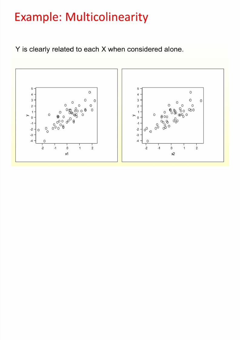
Example: Multicolinearity
8/13/2019 00000chen- Linear Regression Analysis3
http://slidepdf.com/reader/full/00000chen-linear-regression-analysis3 109/252
8/13/2019 00000chen- Linear Regression Analysis3
http://slidepdf.com/reader/full/00000chen-linear-regression-analysis3 110/252

8/13/2019 00000chen- Linear Regression Analysis3
http://slidepdf.com/reader/full/00000chen-linear-regression-analysis3 111/252

8/13/2019 00000chen- Linear Regression Analysis3
http://slidepdf.com/reader/full/00000chen-linear-regression-analysis3 112/252
8/13/2019 00000chen- Linear Regression Analysis3
http://slidepdf.com/reader/full/00000chen-linear-regression-analysis3 113/252
8/13/2019 00000chen- Linear Regression Analysis3
http://slidepdf.com/reader/full/00000chen-linear-regression-analysis3 114/252
8/13/2019 00000chen- Linear Regression Analysis3
http://slidepdf.com/reader/full/00000chen-linear-regression-analysis3 115/252

8/13/2019 00000chen- Linear Regression Analysis3
http://slidepdf.com/reader/full/00000chen-linear-regression-analysis3 116/252
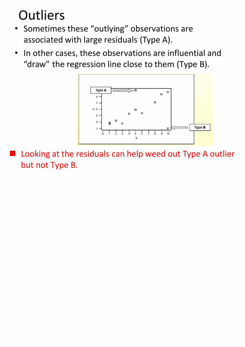
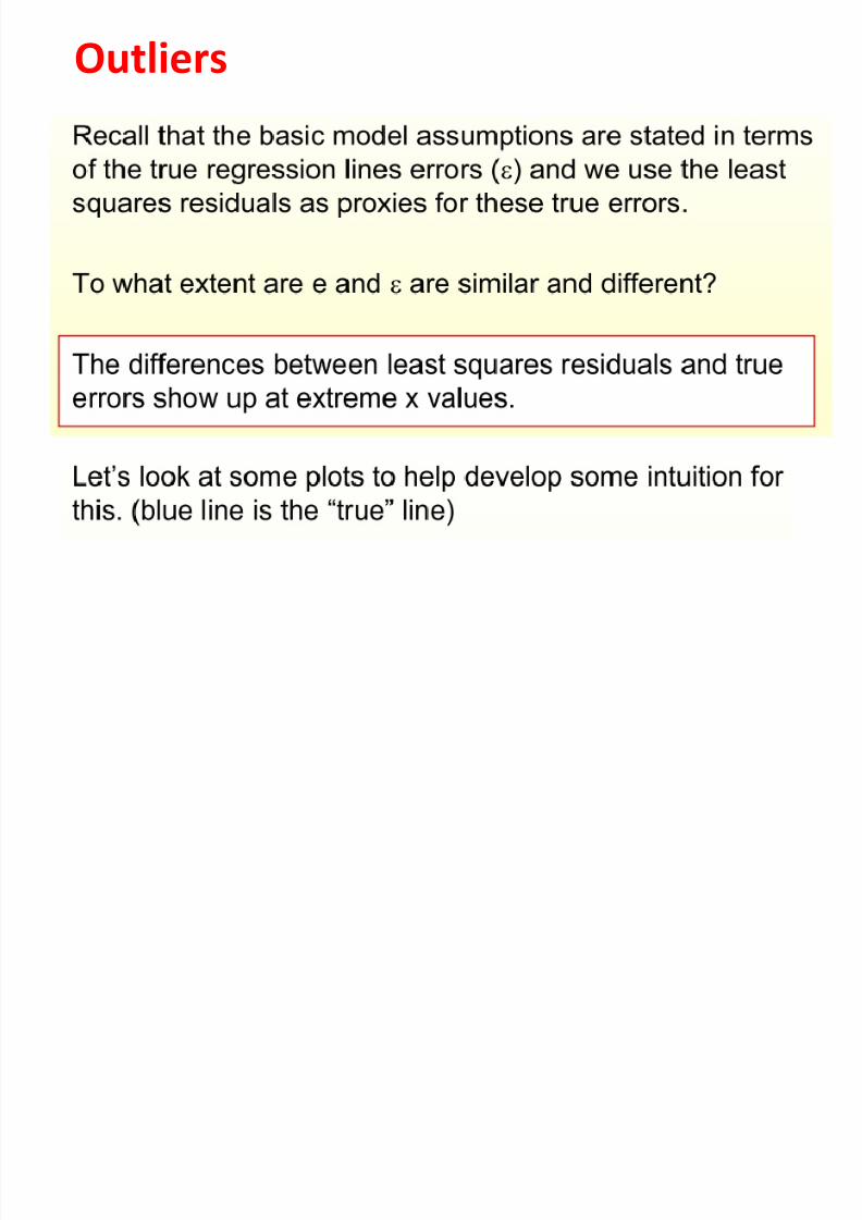
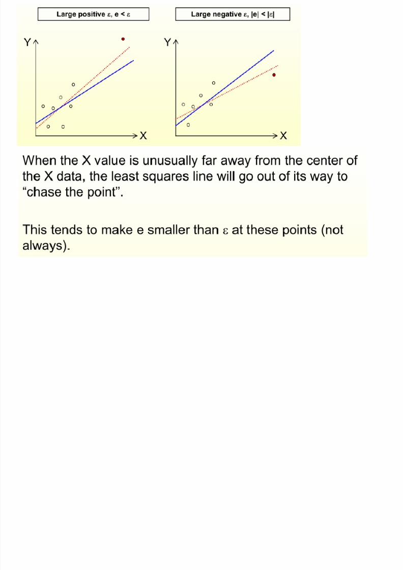
Outliers
Outliers
8/13/2019 00000chen- Linear Regression Analysis3
http://slidepdf.com/reader/full/00000chen-linear-regression-analysis3 117/252

8/13/2019 00000chen- Linear Regression Analysis3
http://slidepdf.com/reader/full/00000chen-linear-regression-analysis3 118/252
8/13/2019 00000chen- Linear Regression Analysis3
http://slidepdf.com/reader/full/00000chen-linear-regression-analysis3 119/252

8/13/2019 00000chen- Linear Regression Analysis3
http://slidepdf.com/reader/full/00000chen-linear-regression-analysis3 120/252
8/13/2019 00000chen- Linear Regression Analysis3
http://slidepdf.com/reader/full/00000chen-linear-regression-analysis3 121/252

8/13/2019 00000chen- Linear Regression Analysis3
http://slidepdf.com/reader/full/00000chen-linear-regression-analysis3 122/252

8/13/2019 00000chen- Linear Regression Analysis3
http://slidepdf.com/reader/full/00000chen-linear-regression-analysis3 123/252
8/13/2019 00000chen- Linear Regression Analysis3
http://slidepdf.com/reader/full/00000chen-linear-regression-analysis3 124/252

8/13/2019 00000chen- Linear Regression Analysis3
http://slidepdf.com/reader/full/00000chen-linear-regression-analysis3 125/252
Outliers = unusual observations
H fi d l b i ?

8/13/2019 00000chen- Linear Regression Analysis3
http://slidepdf.com/reader/full/00000chen-linear-regression-analysis3 126/252
How can we find unusual observations?
cause for outliers

8/13/2019 00000chen- Linear Regression Analysis3
http://slidepdf.com/reader/full/00000chen-linear-regression-analysis3 127/252

8/13/2019 00000chen- Linear Regression Analysis3
http://slidepdf.com/reader/full/00000chen-linear-regression-analysis3 128/252

8/13/2019 00000chen- Linear Regression Analysis3
http://slidepdf.com/reader/full/00000chen-linear-regression-analysis3 129/252

8/13/2019 00000chen- Linear Regression Analysis3
http://slidepdf.com/reader/full/00000chen-linear-regression-analysis3 130/252
8/13/2019 00000chen- Linear Regression Analysis3
http://slidepdf.com/reader/full/00000chen-linear-regression-analysis3 131/252
8/13/2019 00000chen- Linear Regression Analysis3
http://slidepdf.com/reader/full/00000chen-linear-regression-analysis3 132/252

8/13/2019 00000chen- Linear Regression Analysis3
http://slidepdf.com/reader/full/00000chen-linear-regression-analysis3 133/252

8/13/2019 00000chen- Linear Regression Analysis3
http://slidepdf.com/reader/full/00000chen-linear-regression-analysis3 134/252

8/13/2019 00000chen- Linear Regression Analysis3
http://slidepdf.com/reader/full/00000chen-linear-regression-analysis3 135/252

8/13/2019 00000chen- Linear Regression Analysis3
http://slidepdf.com/reader/full/00000chen-linear-regression-analysis3 136/252

8/13/2019 00000chen- Linear Regression Analysis3
http://slidepdf.com/reader/full/00000chen-linear-regression-analysis3 137/252
8/13/2019 00000chen- Linear Regression Analysis3
http://slidepdf.com/reader/full/00000chen-linear-regression-analysis3 138/252
8/13/2019 00000chen- Linear Regression Analysis3
http://slidepdf.com/reader/full/00000chen-linear-regression-analysis3 139/252

8/13/2019 00000chen- Linear Regression Analysis3
http://slidepdf.com/reader/full/00000chen-linear-regression-analysis3 140/252

8/13/2019 00000chen- Linear Regression Analysis3
http://slidepdf.com/reader/full/00000chen-linear-regression-analysis3 141/252

8/13/2019 00000chen- Linear Regression Analysis3
http://slidepdf.com/reader/full/00000chen-linear-regression-analysis3 142/252
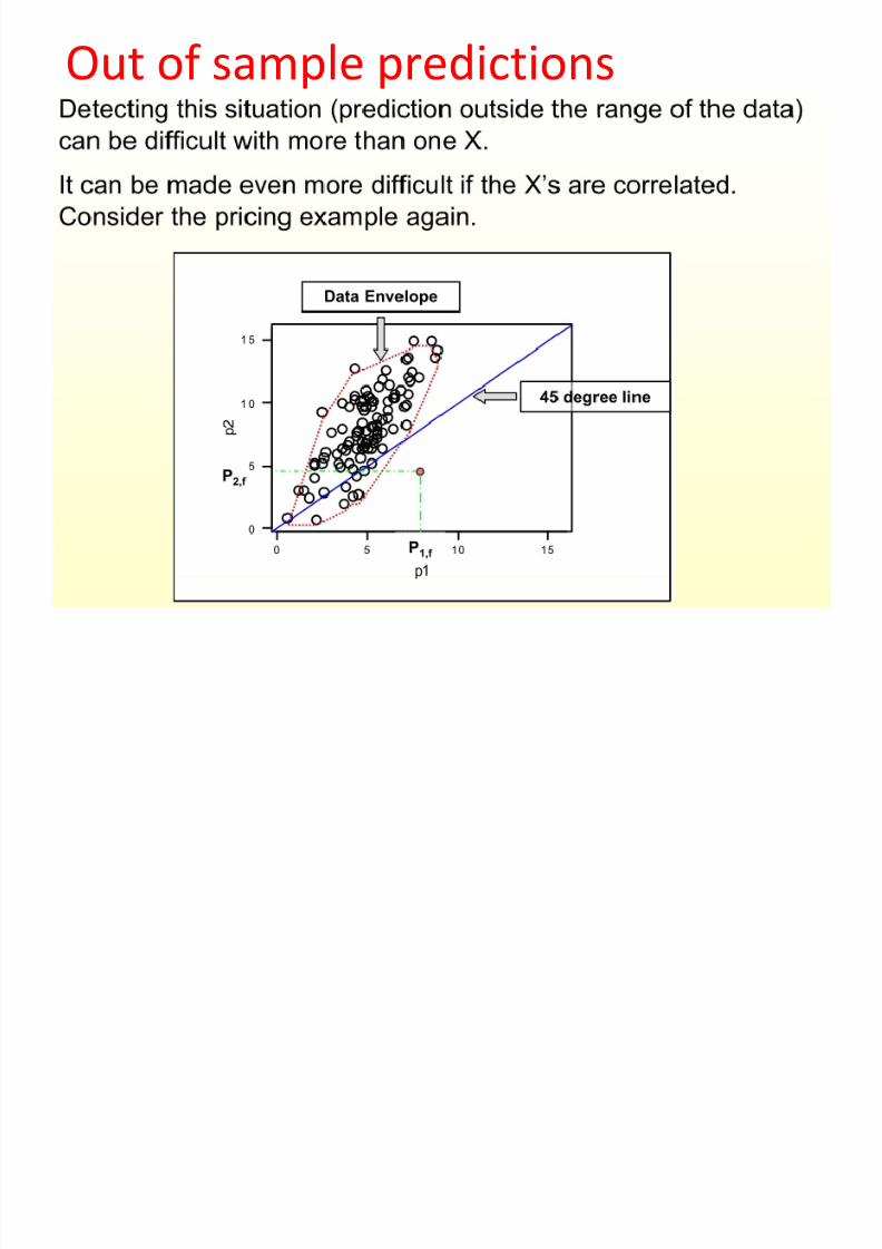
Out of sample predictions

8/13/2019 00000chen- Linear Regression Analysis3
http://slidepdf.com/reader/full/00000chen-linear-regression-analysis3 143/252

8/13/2019 00000chen- Linear Regression Analysis3
http://slidepdf.com/reader/full/00000chen-linear-regression-analysis3 144/252
Out of sample predictions
8/13/2019 00000chen- Linear Regression Analysis3
http://slidepdf.com/reader/full/00000chen-linear-regression-analysis3 145/252
Out of sample-Extrapolation

8/13/2019 00000chen- Linear Regression Analysis3
http://slidepdf.com/reader/full/00000chen-linear-regression-analysis3 146/252
8/13/2019 00000chen- Linear Regression Analysis3
http://slidepdf.com/reader/full/00000chen-linear-regression-analysis3 147/252

8/13/2019 00000chen- Linear Regression Analysis3
http://slidepdf.com/reader/full/00000chen-linear-regression-analysis3 148/252
Non Linear functional forms
• Standard regression model is a linear

8/13/2019 00000chen- Linear Regression Analysis3
http://slidepdf.com/reader/full/00000chen-linear-regression-analysis3 149/252
• Standard regression model is a linear
conditional mean model.• In many situations in practice, it is desirable to
have some flexibility to specify non-linear
regression functions.• The standard linear regression model can be
"tricked" into displaying non-linearity by two
techniques:

8/13/2019 00000chen- Linear Regression Analysis3
http://slidepdf.com/reader/full/00000chen-linear-regression-analysis3 150/252

8/13/2019 00000chen- Linear Regression Analysis3
http://slidepdf.com/reader/full/00000chen-linear-regression-analysis3 151/252

8/13/2019 00000chen- Linear Regression Analysis3
http://slidepdf.com/reader/full/00000chen-linear-regression-analysis3 152/252

8/13/2019 00000chen- Linear Regression Analysis3
http://slidepdf.com/reader/full/00000chen-linear-regression-analysis3 153/252

8/13/2019 00000chen- Linear Regression Analysis3
http://slidepdf.com/reader/full/00000chen-linear-regression-analysis3 154/252

8/13/2019 00000chen- Linear Regression Analysis3
http://slidepdf.com/reader/full/00000chen-linear-regression-analysis3 155/252
8/13/2019 00000chen- Linear Regression Analysis3
http://slidepdf.com/reader/full/00000chen-linear-regression-analysis3 156/252

8/13/2019 00000chen- Linear Regression Analysis3
http://slidepdf.com/reader/full/00000chen-linear-regression-analysis3 157/252
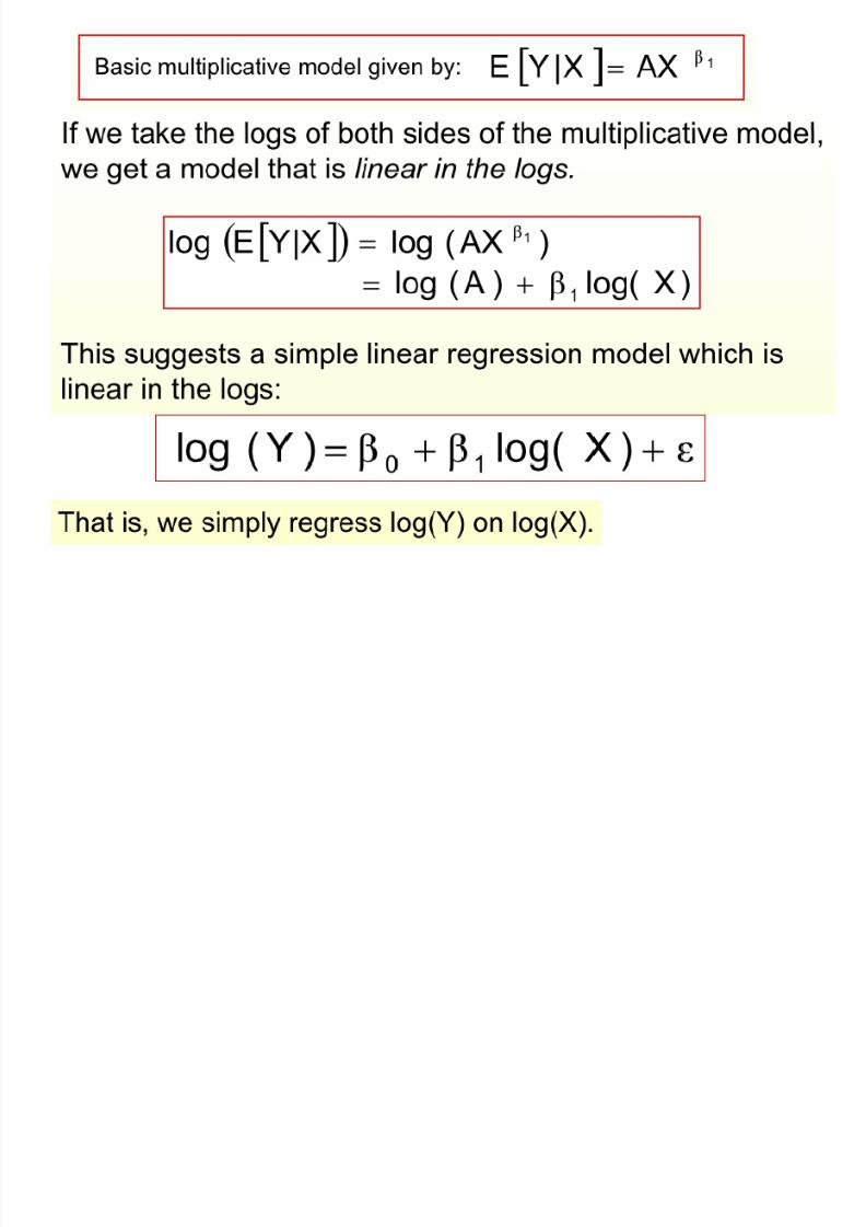
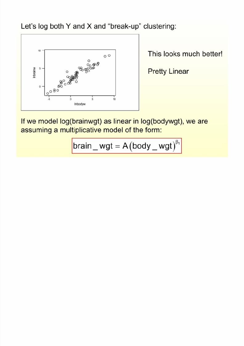
1 1log( ) log( )
Y X
Y X Y X b b
1
log( )log( )
Y
Y Y X X
X
b
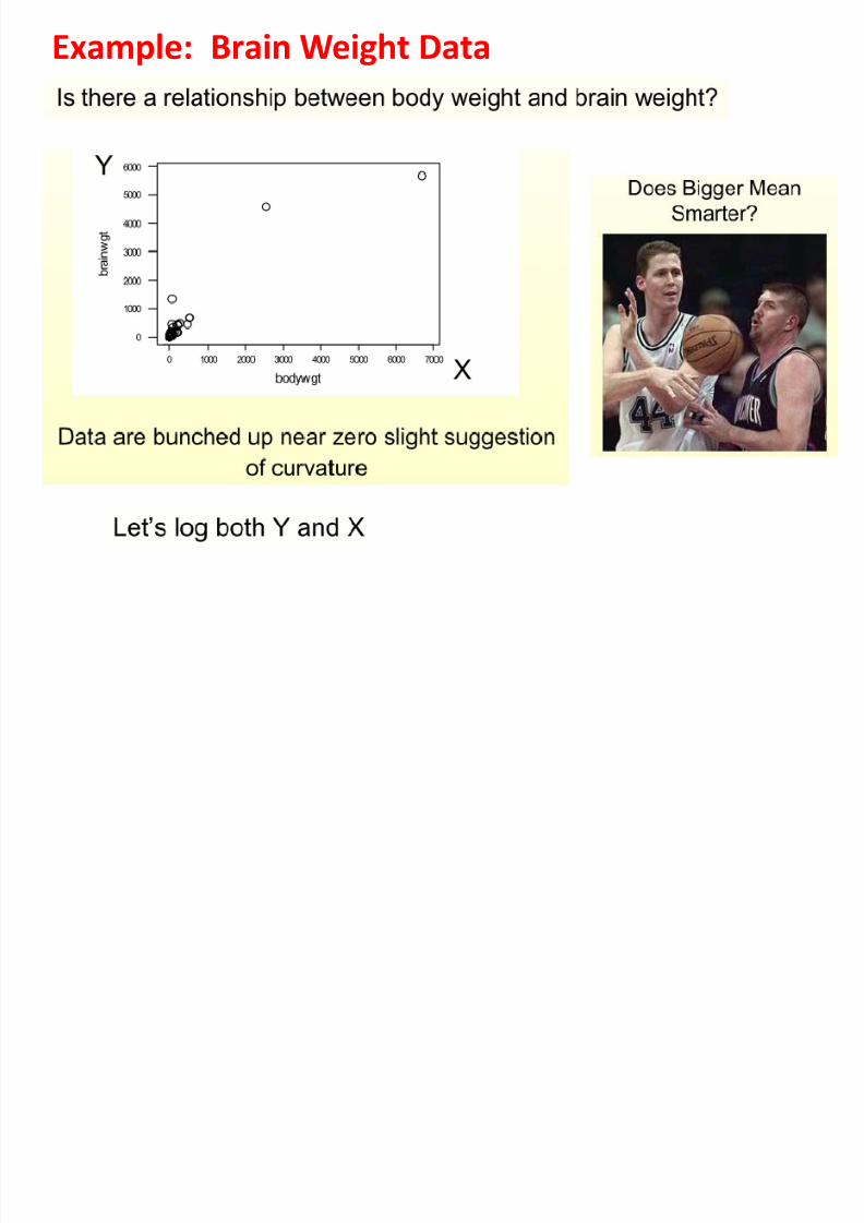
Example: Brain Weight Data
8/13/2019 00000chen- Linear Regression Analysis3
http://slidepdf.com/reader/full/00000chen-linear-regression-analysis3 158/252
8/13/2019 00000chen- Linear Regression Analysis3
http://slidepdf.com/reader/full/00000chen-linear-regression-analysis3 159/252
8/13/2019 00000chen- Linear Regression Analysis3
http://slidepdf.com/reader/full/00000chen-linear-regression-analysis3 160/252

8/13/2019 00000chen- Linear Regression Analysis3
http://slidepdf.com/reader/full/00000chen-linear-regression-analysis3 161/252
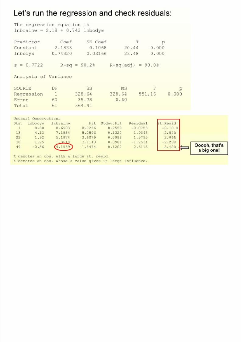
Ln(64)=4.1589
龍貓

8/13/2019 00000chen- Linear Regression Analysis3
http://slidepdf.com/reader/full/00000chen-linear-regression-analysis3 162/252
6.4g<= 64g

8/13/2019 00000chen- Linear Regression Analysis3
http://slidepdf.com/reader/full/00000chen-linear-regression-analysis3 163/252

8/13/2019 00000chen- Linear Regression Analysis3
http://slidepdf.com/reader/full/00000chen-linear-regression-analysis3 164/252

8/13/2019 00000chen- Linear Regression Analysis3
http://slidepdf.com/reader/full/00000chen-linear-regression-analysis3 165/252
Dummy Variables
Categorical Explanatory Variablesin Regression Models

8/13/2019 00000chen- Linear Regression Analysis3
http://slidepdf.com/reader/full/00000chen-linear-regression-analysis3 166/252
166
in Regression Models
• Categorical independent variables can
be incorporated into a regression model
by converting them into 0/1 (“dummy”)
variables
• For binary variables, code dummies “0”
for “no” and 1 for “yes”
Dummy Variables, More than two levels

8/13/2019 00000chen- Linear Regression Analysis3
http://slidepdf.com/reader/full/00000chen-linear-regression-analysis3 167/252
167
For categorical variables with k categories, use
k –1 dummy variables• SMOKE2 has three levels, initially coded
0 = non-smoker , 1 = former smoker, 2 = current smoker
Use k – 1 = 3 – 1 = 2 dummy variables to code
this information like this:

8/13/2019 00000chen- Linear Regression Analysis3
http://slidepdf.com/reader/full/00000chen-linear-regression-analysis3 168/252
Example, cont. • Regress FEV on SMOKE least squares
8/13/2019 00000chen- Linear Regression Analysis3
http://slidepdf.com/reader/full/00000chen-linear-regression-analysis3 169/252
169
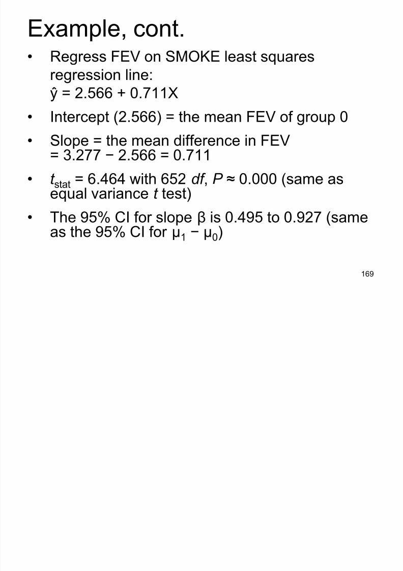
Regress FEV on SMOKE least squares
regression line:ŷ = 2.566 + 0.711X
• Intercept (2.566) = the mean FEV of group 0
• Slope = the mean difference in FEV= 3.277 − 2.566 = 0.711
• t stat = 6.464 with 652 df , P ≈ 0.000 (same asequal variance t test)
• The 95% CI for slope β is 0.495 to 0.927 (sameas the 95% CI for μ1 − μ0)
Dummy Variable SMOKE

8/13/2019 00000chen- Linear Regression Analysis3
http://slidepdf.com/reader/full/00000chen-linear-regression-analysis3 170/252
Basic Biostat 170
Regression linepasses throughgroup means
b = 3.277 – 2.566 = 0.711

8/13/2019 00000chen- Linear Regression Analysis3
http://slidepdf.com/reader/full/00000chen-linear-regression-analysis3 171/252
Multiple RegressionCoefficients

8/13/2019 00000chen- Linear Regression Analysis3
http://slidepdf.com/reader/full/00000chen-linear-regression-analysis3 172/252
172
CoefficientsRely onsoftware to
calculate
multipleregression
statistics

8/13/2019 00000chen- Linear Regression Analysis3
http://slidepdf.com/reader/full/00000chen-linear-regression-analysis3 173/252
Multiple Regression Coefficients, cont.

8/13/2019 00000chen- Linear Regression Analysis3
http://slidepdf.com/reader/full/00000chen-linear-regression-analysis3 174/252
174
• The slope coefficient associated for SMOKE is−0.206, suggesting that smokers have 0.206
less FEV on average compared to non-smokers
(after adjusting for age)
• The slope coefficient for AGE is 0.231,suggesting that each year of age in associated
with an increase of 0.231 FEV units on average
(after adjusting for SMOKE)
Inference About the Coefficients
I f ti l t ti ti l l t d f h

8/13/2019 00000chen- Linear Regression Analysis3
http://slidepdf.com/reader/full/00000chen-linear-regression-analysis3 175/252
175
Coefficientsa
.367 .081 4.511 .000
-.209 .081 -.072 -2.588 .010
.231 .008 .786 28.176 .000
(Constant)
smoke
age
Model
1
B Std. Error
Unstandardized
Coeff icients
Beta
Standardized
Coeff icients
t Sig.
Dependent Variable: feva.
Inferential statistics are calculated for each
regression coefficient. For example, in testing
H 0: β1 = 0 (SMOKE coefficient controlling for AGE)
t stat = −2.588 and P = 0.010
df = n – k – 1 = 654 – 2 – 1 = 651
Inference About the Coefficients
Th 95% fid i t l f thi l f

8/13/2019 00000chen- Linear Regression Analysis3
http://slidepdf.com/reader/full/00000chen-linear-regression-analysis3 176/252
176
The 95% confidence interval for this slope of
SMOKE controlling for AGE is −0.368 to − 0.050.
Coefficientsa
.207 .527
-.368 -.050
.215 .247
(Constant)
smoke
age
Model
1
Lower Bound Upper Bound95% Confidence Interval for B
Dependent Variable: f eva.
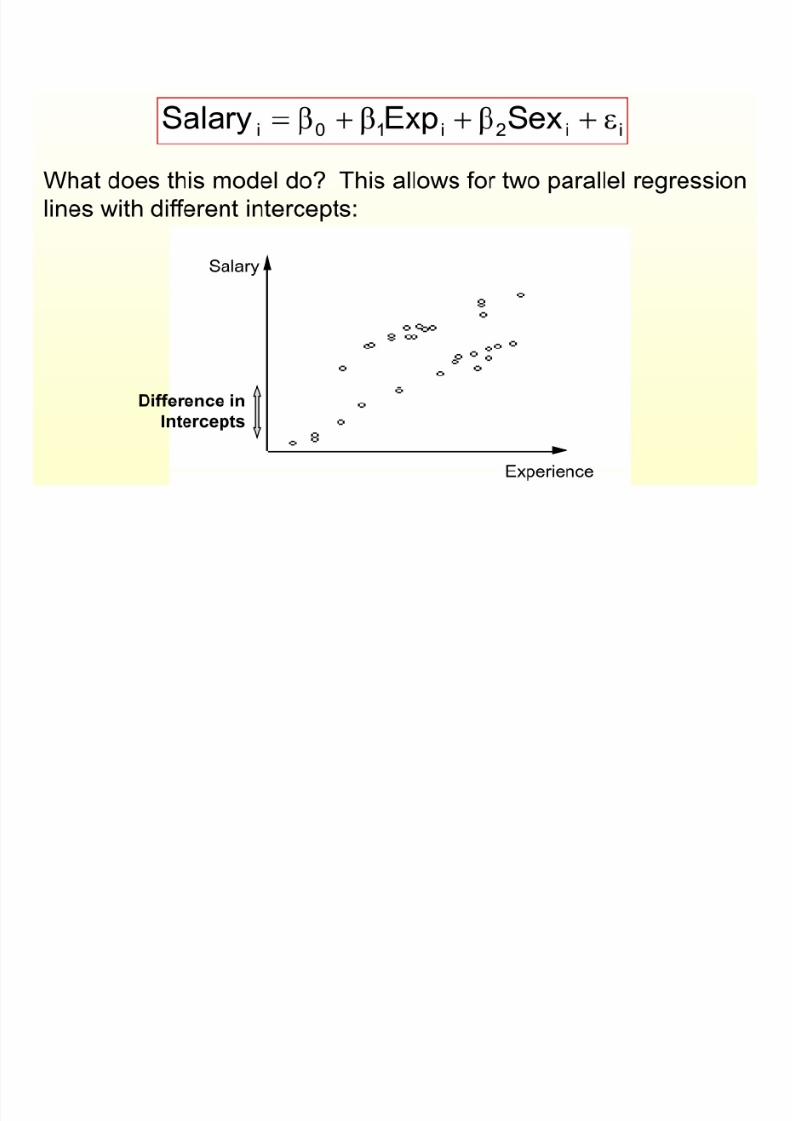
Comparing the Slopes of Two or More Regression Lines
Suppose we have a quantitative explanatory variable, X1, and we have two
possible regression lines: one for situation 1 (location A), the other for situation

8/13/2019 00000chen- Linear Regression Analysis3
http://slidepdf.com/reader/full/00000chen-linear-regression-analysis3 177/252
15-177
Use of dummy (or classification) variables in regression.
y
x1
A)(loc110 x y b b
B)(loc132 x y b b 310 : b b H
200 : b b H
Equal intercepts
Equal slopes
possible regression lines: one for situation 1 (location A), the other for situation
2 (location B).
Reformulate the model.
Define a new variable, x2 such that
x = 0 for situation 1 (Location A)

8/13/2019 00000chen- Linear Regression Analysis3
http://slidepdf.com/reader/full/00000chen-linear-regression-analysis3 178/252
178
x2 = 0 for situation 1 (Location A)
x2 = 1 for situation 2 (Location B)Then use multiple regression.
21322110ˆ x x x x y
When x2=0 we have: 110110ˆ x x y b b
When x2=1 we have:13213120 )()(ˆ x x y b b
Test of 2=0 equivalent to no intercept difference.Test of 3=0 equivalent to no slope difference.
Tests are based on reduction (drop) sums of squares,
as previously defined.
Dummy variable
y y20 and 30 20 and 30
y=0+ 1 x y=0+ 1 x

8/13/2019 00000chen- Linear Regression Analysis3
http://slidepdf.com/reader/full/00000chen-linear-regression-analysis3 179/252
179
x1
x1
y
x1
y
x1
20 and 30 20 and 30
1
y=(0+2)+ (1+3)
x
y=(0+2)+ 1 x
y=0+ 1 x
y=0+ (1+3) x
y=0+ 1 x
y=0+ 1 x

8/13/2019 00000chen- Linear Regression Analysis3
http://slidepdf.com/reader/full/00000chen-linear-regression-analysis3 180/252
Example

8/13/2019 00000chen- Linear Regression Analysis3
http://slidepdf.com/reader/full/00000chen-linear-regression-analysis3 181/252

8/13/2019 00000chen- Linear Regression Analysis3
http://slidepdf.com/reader/full/00000chen-linear-regression-analysis3 182/252
8/13/2019 00000chen- Linear Regression Analysis3
http://slidepdf.com/reader/full/00000chen-linear-regression-analysis3 183/252

8/13/2019 00000chen- Linear Regression Analysis3
http://slidepdf.com/reader/full/00000chen-linear-regression-analysis3 184/252

8/13/2019 00000chen- Linear Regression Analysis3
http://slidepdf.com/reader/full/00000chen-linear-regression-analysis3 185/252

8/13/2019 00000chen- Linear Regression Analysis3
http://slidepdf.com/reader/full/00000chen-linear-regression-analysis3 186/252

8/13/2019 00000chen- Linear Regression Analysis3
http://slidepdf.com/reader/full/00000chen-linear-regression-analysis3 187/252
8/13/2019 00000chen- Linear Regression Analysis3
http://slidepdf.com/reader/full/00000chen-linear-regression-analysis3 188/252
Example

8/13/2019 00000chen- Linear Regression Analysis3
http://slidepdf.com/reader/full/00000chen-linear-regression-analysis3 189/252
8/13/2019 00000chen- Linear Regression Analysis3
http://slidepdf.com/reader/full/00000chen-linear-regression-analysis3 190/252

8/13/2019 00000chen- Linear Regression Analysis3
http://slidepdf.com/reader/full/00000chen-linear-regression-analysis3 191/252

8/13/2019 00000chen- Linear Regression Analysis3
http://slidepdf.com/reader/full/00000chen-linear-regression-analysis3 192/252
Autocorrelation
in the errors
8/13/2019 00000chen- Linear Regression Analysis3
http://slidepdf.com/reader/full/00000chen-linear-regression-analysis3 193/252
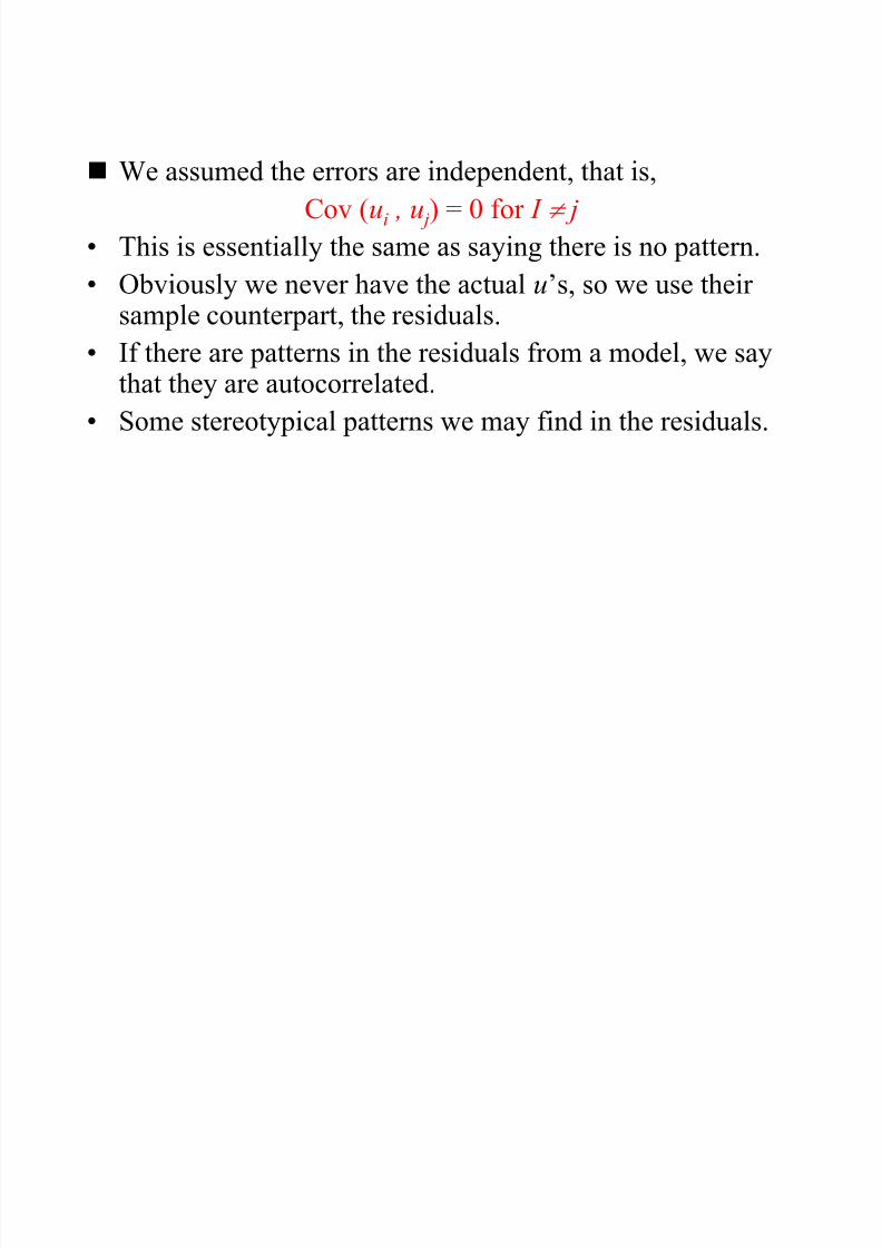
We assumed the errors are independent, that is,Cov (ui , u j) = 0 for I j
• This is essentially the same as saying there is no pattern.
• Obviously we never have the actual u’s, so we use theirsample counterpart, the residuals.
• If there are patterns in the residuals from a model, we saythat they are autocorrelated.
• Some stereotypical patterns we may find in the residuals.
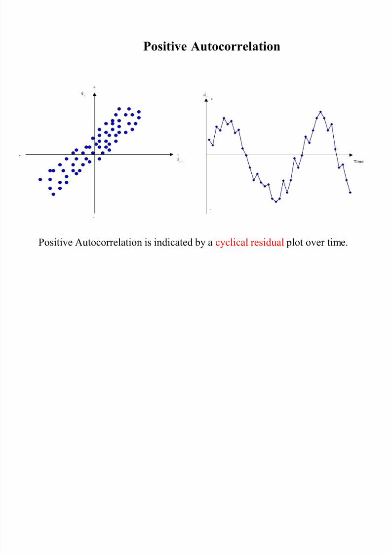
Positive Autocorrelation
8/13/2019 00000chen- Linear Regression Analysis3
http://slidepdf.com/reader/full/00000chen-linear-regression-analysis3 194/252
Positive Autocorrelation is indicated by a cyclical residual plot over time.
+
-
-
t ˆ
+
1ˆ
t
+
-
Time
t u
Negative Autocorrelation

8/13/2019 00000chen- Linear Regression Analysis3
http://slidepdf.com/reader/full/00000chen-linear-regression-analysis3 195/252
Negative autocorrelation is indicated by an alternating pattern where the residuals
cross the time axis more frequently than if they were distributed randomly
+
-
-
t u
+
1ˆ
t u
+
-
t u
Time
No pattern in residuals –
No autocorrelation

8/13/2019 00000chen- Linear Regression Analysis3
http://slidepdf.com/reader/full/00000chen-linear-regression-analysis3 196/252
No pattern in residuals at all: this is what we would like to see
+
t u
-
-
+
1ˆ t
+
t uˆ
Detecting Autocorrelation:
The Durbin-Watson Test
8/13/2019 00000chen- Linear Regression Analysis3
http://slidepdf.com/reader/full/00000chen-linear-regression-analysis3 197/252
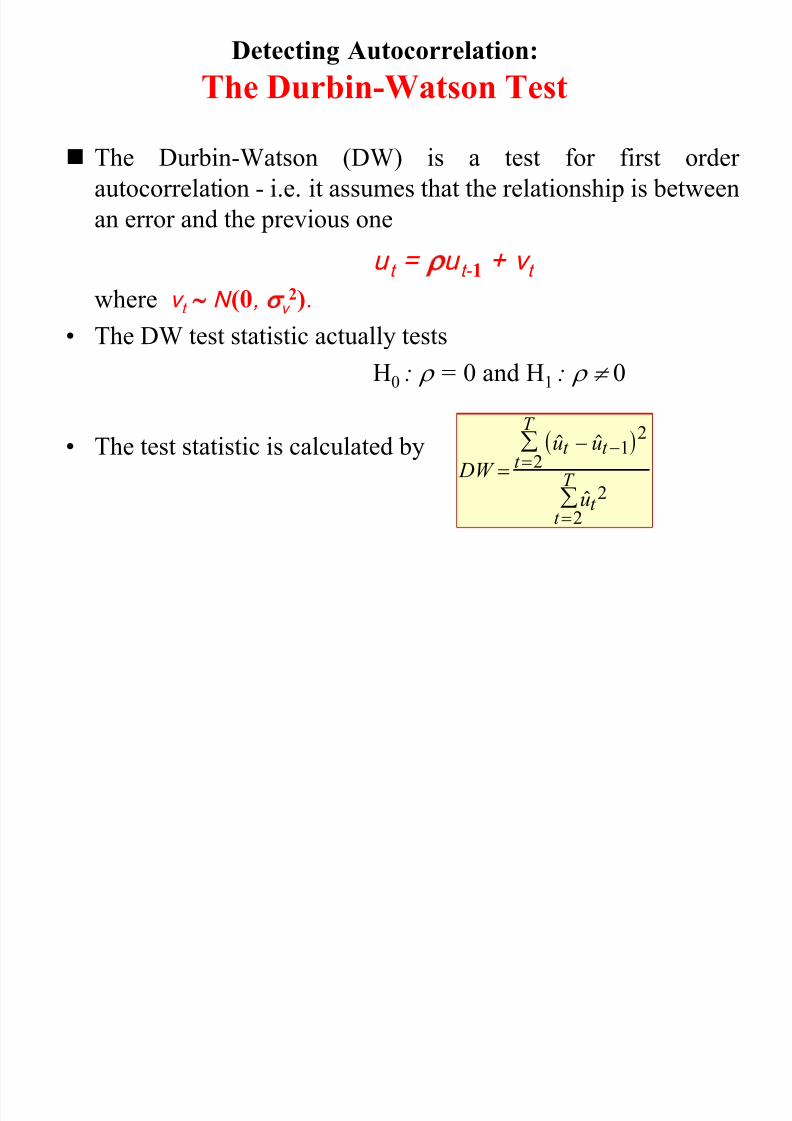
The Durbin-Watson (DW) is a test for first orderautocorrelation - i.e. it assumes that the relationship is between
an error and the previous one
u t = u t- 1 + v t
where v t N (0, v 2).• The DW test statistic actually tests
H0 : = 0 and H1 : 0
• The test statistic is calculated by DW
u u
u
t t t
T
t t
T
1 22
2
2
The Durbin-Watson Test: Critical Values
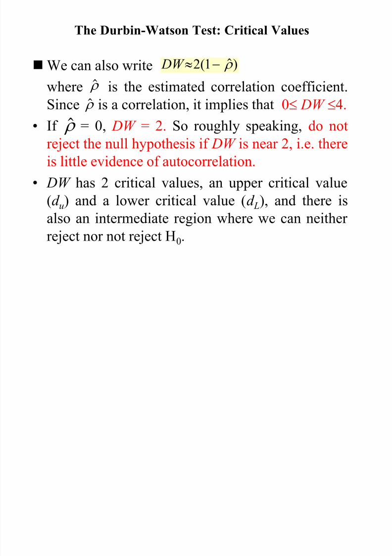
We can also write DW 2 1( )
8/13/2019 00000chen- Linear Regression Analysis3
http://slidepdf.com/reader/full/00000chen-linear-regression-analysis3 198/252
where is the estimated correlation coefficient.Since is a correlation, it implies that 0 DW 4.
• If = 0, DW = 2. So roughly speaking, do not
reject the null hypothesis if DW is near 2, i.e. thereis little evidence of autocorrelation.
• DW has 2 critical values, an upper critical value
(d u) and a lower critical value (d L), and there is
also an intermediate region where we can neitherreject nor not reject H0.
( )
The Durbin-Watson Test: Interpreting the Results
8/13/2019 00000chen- Linear Regression Analysis3
http://slidepdf.com/reader/full/00000chen-linear-regression-analysis3 199/252
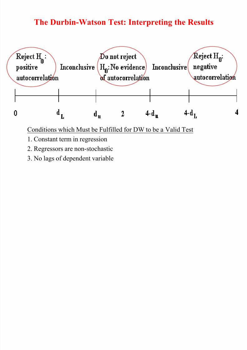
Conditions which Must be Fulfilled for DW to be a Valid Test
1. Constant term in regression
2. Regressors are non-stochastic
3. No lags of dependent variable
Another Test for Autocorrelation:
The Breusch-Godfrey Test

8/13/2019 00000chen- Linear Regression Analysis3
http://slidepdf.com/reader/full/00000chen-linear-regression-analysis3 200/252
• It is a more general test for r th order autocorrelation:
N(0, )
• The null and alternative hypotheses are:
H0 : 1 = 0 and 2 = 0 and ... and r = 0
H1 : 1 0 or 2 0 or ... or r 0• The test is carried out as follows:
1). Estimate the linear regression using OLS and obtain the residuals,
2). Regress on all of the regressors from stage 1 (the x’s) plus
Obtain R2 from this regression.
3). It can be shown that (T-r )R 2 2(r )
• If the test statistic exceeds the critical value from the statistical tables,
reject the null hypothesis of no autocorrelation.
ut
ut
u u u u u v vt t t t r t r t t 1 1 2 2 3 3 ... ,
, ,..., u u ut t t r 1 2
2
v
Consequences of Ignoring Autocorrelation
if it is Present
8/13/2019 00000chen- Linear Regression Analysis3
http://slidepdf.com/reader/full/00000chen-linear-regression-analysis3 201/252
• The coefficient estimates derived using OLS are stillunbiased, but they are inefficient, i.e. they are not BLUE,
even in large sample sizes.
• Thus, if the standard error estimates are inappropriate,
there exists the possibility that we could make the wronginferences.
• R2 is likely to be inflated relative to its “correct” value for
positively correlated residuals.
“Remedies” for Autocorrelation

8/13/2019 00000chen- Linear Regression Analysis3
http://slidepdf.com/reader/full/00000chen-linear-regression-analysis3 202/252
• If the form of the autocorrelation is known, we could use a GLS procedure – i.e. an approach that allows for autocorrelated residualse.g., Cochrane-Orcutt.
• But such procedures that “correct” for autocorrelation requireassumptions about the form of the autocorrelation.
• If these assumptions are invalid, the cure would be more dangerousthan the disease! - see Hendry and Mizon (1978).
• However, it is unlikely to be the case that the form of theautocorrelation is known, and a more “modern” view is that residualautocorrelation presents an opportunity to modify the regression.
Dynamic Models

8/13/2019 00000chen- Linear Regression Analysis3
http://slidepdf.com/reader/full/00000chen-linear-regression-analysis3 203/252
• All of the models we have considered so far have been static, e.g.
yt = b 1 + b 2 x2t + ... + b k xkt + ut
• But we can easily extend this analysis to the case where the current
value of yt
depends on previous values of y or one of the x’s, e.g.
yt = b 1 + b 2 x2t + ... + b k xkt + 1 yt -1 + 2 x2t -1 + … + k xkt -1+ ut
• We could extend the model even further by adding extra lags, e.g.
x2t-2 , yt-3 .
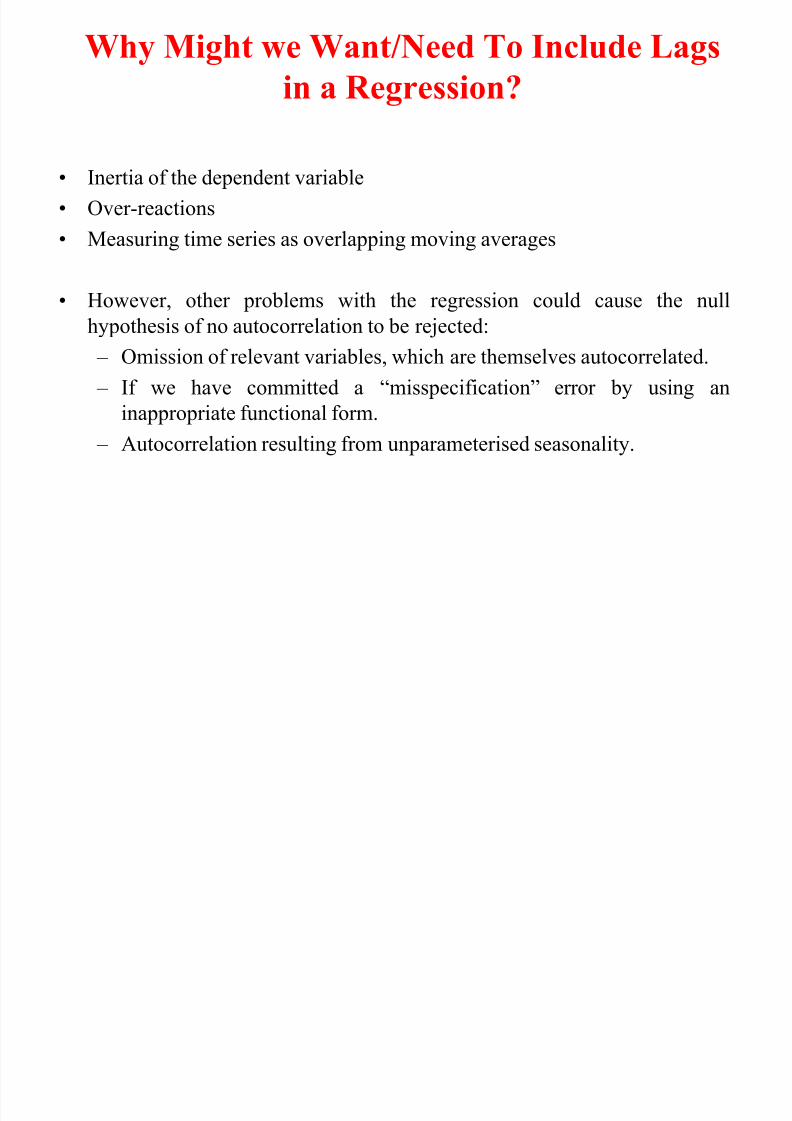
Why Might we Want/Need To Include Lags
in a Regression?
8/13/2019 00000chen- Linear Regression Analysis3
http://slidepdf.com/reader/full/00000chen-linear-regression-analysis3 204/252
• Inertia of the dependent variable
• Over-reactions
• Measuring time series as overlapping moving averages
• However, other problems with the regression could cause the nullhypothesis of no autocorrelation to be rejected:
– Omission of relevant variables, which are themselves autocorrelated.
– If we have committed a “misspecification” error by using an
inappropriate functional form.
– Autocorrelation resulting from unparameterised seasonality.

8/13/2019 00000chen- Linear Regression Analysis3
http://slidepdf.com/reader/full/00000chen-linear-regression-analysis3 205/252

8/13/2019 00000chen- Linear Regression Analysis3
http://slidepdf.com/reader/full/00000chen-linear-regression-analysis3 206/252
The Long Run Static Equilibrium Solution:
An Example

8/13/2019 00000chen- Linear Regression Analysis3
http://slidepdf.com/reader/full/00000chen-linear-regression-analysis3 207/252
If our model is
yt = b 1 + b 2 x2t + b 3 x2t -1 + b 4 yt -1 + ut
then the static solution would be given by0 = b 1 + b 3 x2t -1 + b 4 yt -1
b4 yt -1 = - b 1 - b 3 x2t -1
2
4
3
4
1 x y b b
b b
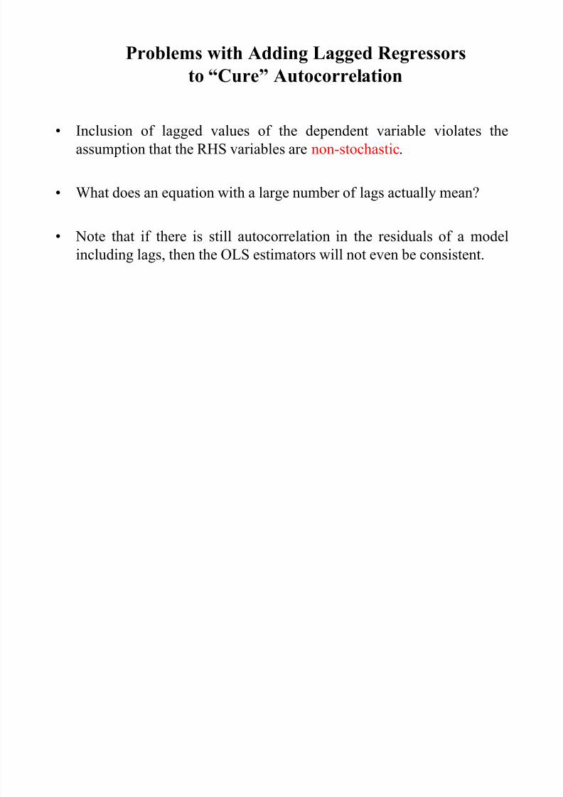
Problems with Adding Lagged Regressors
to “Cure” Autocorrelation
8/13/2019 00000chen- Linear Regression Analysis3
http://slidepdf.com/reader/full/00000chen-linear-regression-analysis3 208/252
• Inclusion of lagged values of the dependent variable violates the
assumption that the RHS variables are non-stochastic.
• What does an equation with a large number of lags actually mean?
• Note that if there is still autocorrelation in the residuals of a model
including lags, then the OLS estimators will not even be consistent.

8/13/2019 00000chen- Linear Regression Analysis3
http://slidepdf.com/reader/full/00000chen-linear-regression-analysis3 209/252

8/13/2019 00000chen- Linear Regression Analysis3
http://slidepdf.com/reader/full/00000chen-linear-regression-analysis3 210/252

8/13/2019 00000chen- Linear Regression Analysis3
http://slidepdf.com/reader/full/00000chen-linear-regression-analysis3 211/252
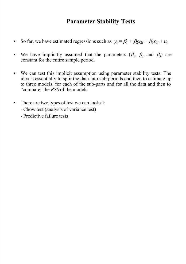
Parameter Stability Tests
Parameter Stability Tests
8/13/2019 00000chen- Linear Regression Analysis3
http://slidepdf.com/reader/full/00000chen-linear-regression-analysis3 212/252
• So far, we have estimated regressions such as
• We have implicitly assumed that the parameters ( b 1, b 2 and b 3) areconstant for the entire sample period.
• We can test this implicit assumption using parameter stability tests. Theidea is essentially to split the data into sub-periods and then to estimate upto three models, for each of the sub-parts and for all the data and then to“compare” the RSS of the models.
• There are two types of test we can look at:- Chow test (analysis of variance test)
- Predictive failure tests
t = b 1 + b 2 x2t + b 3 x3t + ut
The Chow Test

8/13/2019 00000chen- Linear Regression Analysis3
http://slidepdf.com/reader/full/00000chen-linear-regression-analysis3 213/252
• The steps involved are:
1. Split the data into two sub-periods. Estimate the regression over the
whole period and then for the two sub-periods separately (3 regressions).
Obtain the RSS for each regression.
2. The restricted regression is now the regression for the whole period
while the “unrestricted regression” comes in two parts: for each of the sub-
samples.
We can thus form an F-test which is the difference between the RSS ’s.
The statistic is
RSS RSS RSS
RSS RSS T k
k
1 2
1 2
2
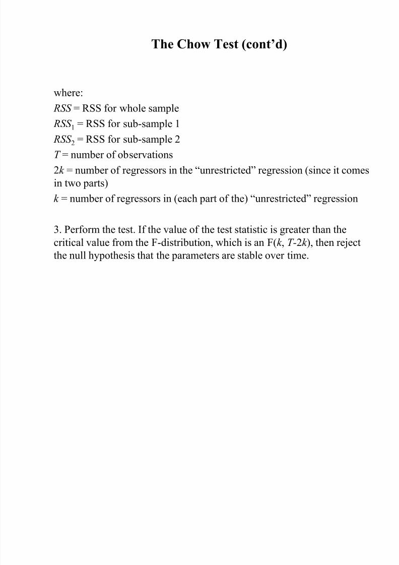
The Chow Test (cont’d)
8/13/2019 00000chen- Linear Regression Analysis3
http://slidepdf.com/reader/full/00000chen-linear-regression-analysis3 214/252
where:
RSS = RSS for whole sample
RSS 1 = RSS for sub-sample 1
RSS 2 = RSS for sub-sample 2
T = number of observations2k = number of regressors in the “unrestricted” regression (since it comes
in two parts)
k = number of regressors in (each part of the) “unrestricted” regression
3. Perform the test. If the value of the test statistic is greater than the
critical value from the F-distribution, which is an F(k , T-2k ), then reject
the null hypothesis that the parameters are stable over time.
A Chow Test Example

8/13/2019 00000chen- Linear Regression Analysis3
http://slidepdf.com/reader/full/00000chen-linear-regression-analysis3 215/252
• Consider the following regression for the CAPM b (again) for the
returns on Glaxo.
• Say that we are interested in estimating Beta for monthly data from
1981-1992. The model for each sub-period is
• 1981M1 - 1987M10
0.24 + 1.2 R Mt T = 82 RSS 1 = 0.03555
• 1987M11 - 1992M12
0.68 + 1.53 R Mt T = 62 RSS 2 = 0.00336
• 1981M1 - 1992M12
0.39 + 1.37 R Mt T = 144 RSS = 0.0434
A Chow Test Example - Results
8/13/2019 00000chen- Linear Regression Analysis3
http://slidepdf.com/reader/full/00000chen-linear-regression-analysis3 216/252
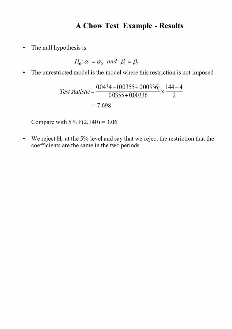
• The null hypothesis is
• The unrestricted model is the model where this restriction is not imposed
= 7.698
Compare with 5% F(2,140) = 3.06
• We reject H0 at the 5% level and say that we reject the restriction that thecoefficients are the same in the two periods.
H and 0 1 2 1 2: b b
Test statistic 00434 00355 000336
0 0355 0 00336
144 4
2
. . .
. .
The Predictive Failure Test

8/13/2019 00000chen- Linear Regression Analysis3
http://slidepdf.com/reader/full/00000chen-linear-regression-analysis3 217/252
• Problem with the Chow test is that we need to have enough data to do theregression on both sub-samples, i.e. T 1>>k , T 2>>k .
• An alternative formulation is the predictive failure test.
• What we do with the predictive failure test is estimate the regression over a “long” sub-period (i.e. most of the data) and then we predict values for the other periodand compare the two.
To calculate the test:
- Run the regression for the whole period (the restricted regression) and obtain the RSS
- Run the regression for the “large” sub-period and obtain the RSS (called RSS 1). Note
we call the number of observations T 1 (even though it may come second).
where T 2 = number of observations we are attempting to “predict”. The test statistic
will follow an F(T 2, T 1-k ).
2
1
1
1StatisticTestT
k T
RSS
RSS RSS
Backwards versus Forwards Predictive Failure Tests

8/13/2019 00000chen- Linear Regression Analysis3
http://slidepdf.com/reader/full/00000chen-linear-regression-analysis3 218/252
• There are 2 types of predictive failure tests:
- Forward predictive failure tests, where we keep the last few
observations back for forecast testing, e.g. we have observations for
1970Q1-1994Q4. So estimate the model over 1970Q1-1993Q4 andforecast 1994Q1-1994Q4.
- Backward predictive failure tests, where we attempt to “back -cast”
the first few observations, e.g. if we have data for 1970Q1-1994Q4,
and we estimate the model over 1971Q1-1994Q4 and backcast1970Q1-1970Q4.

8/13/2019 00000chen- Linear Regression Analysis3
http://slidepdf.com/reader/full/00000chen-linear-regression-analysis3 219/252

8/13/2019 00000chen- Linear Regression Analysis3
http://slidepdf.com/reader/full/00000chen-linear-regression-analysis3 220/252
Omission of an Important Variable or
Inclusion of an Irrelevant Variable

8/13/2019 00000chen- Linear Regression Analysis3
http://slidepdf.com/reader/full/00000chen-linear-regression-analysis3 221/252
Omission of an Important Variable
• Consequence: The estimated coefficients on all the other variables will be biased and inconsistent unless the excluded variable is uncorrelated withall the included variables.
• Even if this condition is satisfied, the estimate of the coefficient on theconstant term will be biased.
• The standard errors will also be biased.
Inclusion of an Irrelevant Variable
• Coefficient estimates will still be consistent and unbiased, but theestimators will be inefficient.
How do we decide the sub-parts to use?
8/13/2019 00000chen- Linear Regression Analysis3
http://slidepdf.com/reader/full/00000chen-linear-regression-analysis3 222/252
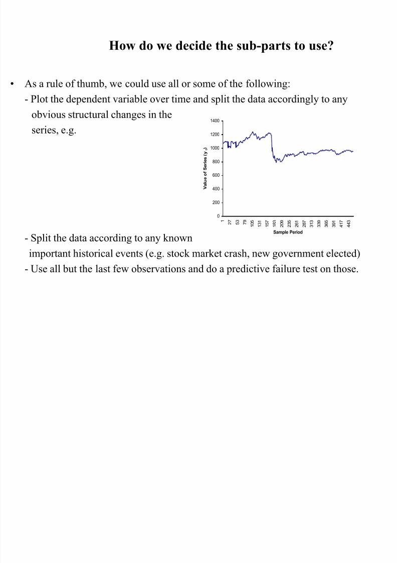
• As a rule of thumb, we could use all or some of the following:- Plot the dependent variable over time and split the data accordingly to any
obvious structural changes in the
series, e.g.
- Split the data according to any known
important historical events (e.g. stock market crash, new government elected)
- Use all but the last few observations and do a predictive failure test on those.
0
200
400
600
800
1000
1200
1400
1 2 7 5 3 7 9
1 0 5
1 3 1
1 5 7
1 8 3
2 0 9
2 3 5
2 6 1
2 8 7
3 1 3
3 3 9
3 6 5
3 9 1
4 1 7
4 4 3
Sample Period
V a l u e o f S e r i e s ( y t )
A Strategy for Building Econometric Models

8/13/2019 00000chen- Linear Regression Analysis3
http://slidepdf.com/reader/full/00000chen-linear-regression-analysis3 223/252
Our Objective:
• To build a statistically adequate empirical model which
- satisfies the assumptions of the CLRM
- is parsimonious
- has the appropriate theoretical interpretation
- has the right “shape” - i.e.
- all signs on coefficients are “correct”
- all sizes of coefficients are “correct”
- is capable of explaining the results of all competing models
2 Approaches to Building Econometric Models

8/13/2019 00000chen- Linear Regression Analysis3
http://slidepdf.com/reader/full/00000chen-linear-regression-analysis3 224/252
• There are 2 popular philosophies of building econometric models: the“specific-to-general” and “general-to-specific” approaches.
• “Specific-to-general” was used almost universally until the mid 1980’s, and involved starting with the simplest model and gradually adding to it.
• Little, if any, diagnostic testing was undertaken. But this meant that allinferences were potentially invalid.
• An alternative and more modern approach to model building is the “LSE”
or Hendry “general-to-specific” methodology.
• The advantages of this approach are that it is statistically sensible and alsothe theory on which the models are based usually has nothing to say aboutthe lag structure of a model.
The General-to-Specific Approach

8/13/2019 00000chen- Linear Regression Analysis3
http://slidepdf.com/reader/full/00000chen-linear-regression-analysis3 225/252
• First step is to form a “large” model with lots of variables on the right handside
• This is known as a GUM (generalised unrestricted model)
• At this stage, we want to make sure that the model satisfies all of the
assumptions of the CLRM
• If the assumptions are violated, we need to take appropriate actions to remedythis, e.g.
- taking logs
- adding lags
- dummy variables
• We need to do this before testing hypotheses
• Once we have a model which satisfies the assumptions, it could be very big
with lots of lags & independent variables
The General-to-Specific Approach:
Reparameterising the Model
8/13/2019 00000chen- Linear Regression Analysis3
http://slidepdf.com/reader/full/00000chen-linear-regression-analysis3 226/252
• The next stage is to reparameterise the model by
- knocking out very insignificant regressors
- some coefficients may be insignificantly different from each other,
so we can combine them.
• At each stage, we need to check the assumptions are still OK.
• Hopefully at this stage, we have a statistically adequate empirical model
which we can use for
- testing underlying financial theories
- forecasting future values of the dependent variable
- formulating policies, etc.
Regression Analysis In Practice - A Further Example:
Determinants of Sovereign Credit Ratings
8/13/2019 00000chen- Linear Regression Analysis3
http://slidepdf.com/reader/full/00000chen-linear-regression-analysis3 227/252
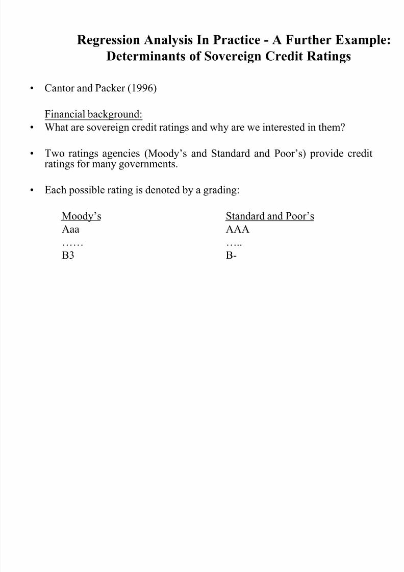
• Cantor and Packer (1996)
Financial background:
• What are sovereign credit ratings and why are we interested in them?
• Two ratings agencies (Moody’s and Standard and Poor’s) provide creditratings for many governments.
• Each possible rating is denoted by a grading:
Moody’s Standard and Poor’s
Aaa AAA…… …..
B3 B-
Purposes

8/13/2019 00000chen- Linear Regression Analysis3
http://slidepdf.com/reader/full/00000chen-linear-regression-analysis3 228/252
- to attempt to explain and model how the ratings agencies arrived at
their ratings.
- to use the same factors to explain the spreads of sovereign yields
above a risk-free proxy
- to determine what factors affect how the sovereign yields react to
ratings announcements
Determinants of Sovereign Ratings
• Data

8/13/2019 00000chen- Linear Regression Analysis3
http://slidepdf.com/reader/full/00000chen-linear-regression-analysis3 229/252
Data
Quantifying the ratings (dependent variable): Aaa/AAA=16, ... , B3/B-=1
• Explanatory variables (units of measurement):
- Per capita income in 1994 (thousands of dollars)
- Average annual GDP growth 1991-1994 (%)
- Average annual inflation 1992-1994 (%)
- Fiscal balance: Average annual government budget surplus as a
proportion of GDP 1992-1994 (%)
- External balance: Average annual current account surplus as a proportion
of GDP 1992-1994 (%)
- External debt Foreign currency debt as a proportion of exports 1994 (%)
- Dummy for economic development
- Dummy for default history
Income and inflation are transformed to their logarithms.
The model: Linear and estimated using OLS

8/13/2019 00000chen- Linear Regression Analysis3
http://slidepdf.com/reader/full/00000chen-linear-regression-analysis3 230/252
Dependent Variable
Explanatory VariableExpected
signAverageRating
Moody’sRating
S&PRating
Moody’s / S&PDifference
Intercept ? 1.442(0.663)
3.408(1.379)
-0.524(-0.223)
3.932**(2.521)
Per capita income + 1.242***(5.302)
1.027***(4.041)
1.458***(6.048)
-0.431***(-2.688)
GDP growth + 0.151(1.935)
0.130(1.545)
0.171**(2.132)
-0.040(0.756)
Inflation - -0.611***(-2.839)
-0.630***(-2.701)
-0.591***(2.671)
-0.039(-0.265)
Fiscal Balance + 0.073(1.324)
0.049(0.818)
0.097*(1.71)
-0.048(-1.274)
External Balance + 0.003(0.314)
0.006(0.535)
0.001(0.046)
0.006(0.779)
External Debt - -0.013***(-5.088)
-0.015***(-5.365)
-0.011***(-4.236)
-0.004***(-2.133)
Development dummy + 2.776***
(4.25)
2.957***
(4.175)
2.595***
(3.861)
0.362
(0.81)Default dummy - -2.042***
(-3.175)-1.63**(-2.097)
-2.622***(-3.962)
1.159***(2.632)
Adjusted R2 0.924 0.905 0.926 0.836 Notes: t -ratios in parentheses; *, **, and *** indicate significance at the 10%, 5% and 1% levelsrespectively. Source: Cantor and Packer (1996). Reprinted with permission from Institutional Investor .
Interpreting the Model

8/13/2019 00000chen- Linear Regression Analysis3
http://slidepdf.com/reader/full/00000chen-linear-regression-analysis3 231/252
From a statistical perspective • Virtually no diagnostics
• Adjusted R2 is high
• Look at the residuals: actual rating - fitted rating
From a financial perspective
• Do the coefficients have their expected signs and sizes?
Do Ratings Add to Publicly Available Available Information?• Now dependent variable is
- Log (Yield on the sovereign bond - yield on a US treasury bond)
Do Ratings Add to Publicly Available Available
Information? Results
Dependent Variable: Log (yield spread)
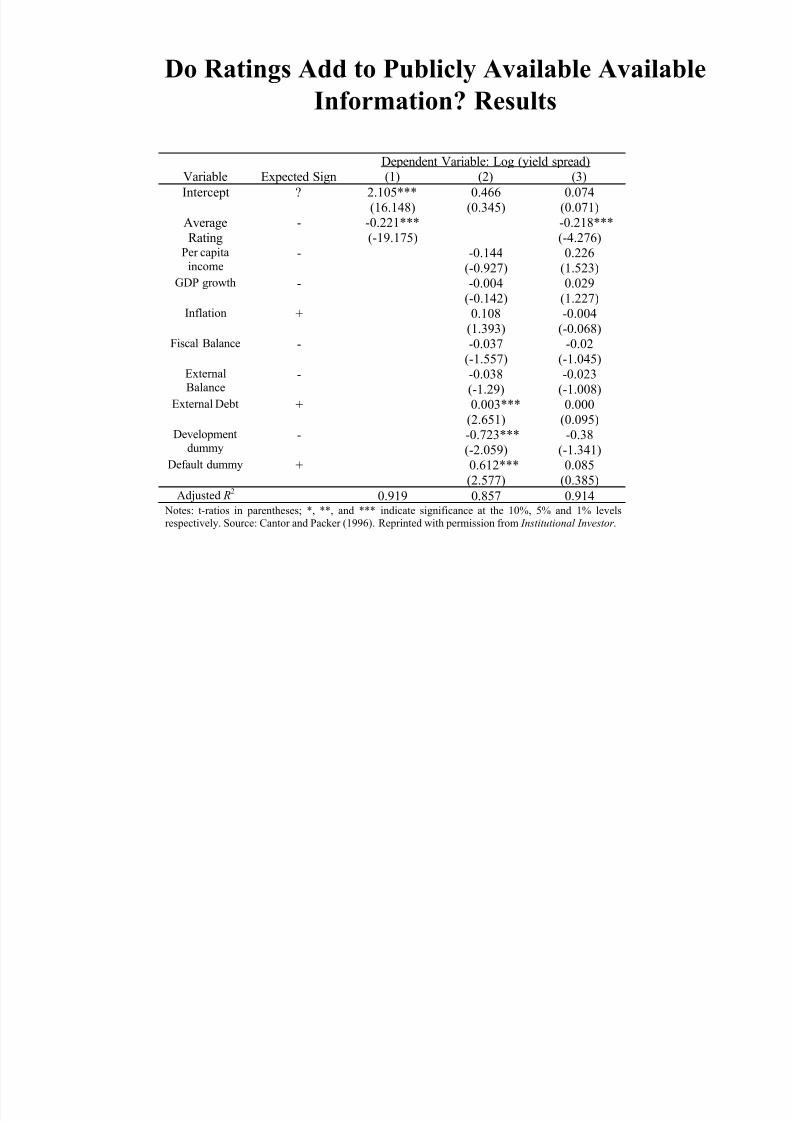
8/13/2019 00000chen- Linear Regression Analysis3
http://slidepdf.com/reader/full/00000chen-linear-regression-analysis3 232/252
p g (y p )
Variable Expected Sign (1) (2) (3)Intercept ? 2.105***
(16.148)
0.466
(0.345)
0.074
(0.071)
Average
Rating
- -0.221***
(-19.175)
-0.218***
(-4.276)Per capita
income- -0.144
(-0.927)
0.226
(1.523)GDP growth - -0.004
(-0.142)
0.029
(1.227)Inflation + 0.108
(1.393)
-0.004
(-0.068)Fiscal Balance - -0.037
(-1.557)
-0.02
(-1.045)ExternalBalance
- -0.038
(-1.29)
-0.023
(-1.008)External Debt + 0.003***
(2.651)
0.000
(0.095)Development
dummy- -0.723***
(-2.059)
-0.38
(-1.341)Default dummy + 0.612***
(2.577)
0.085
(0.385)Adjusted R
20.919 0.857 0.914
Notes: t-ratios in parentheses; *, **, and *** indicate significance at the 10%, 5% and 1% levels
respectively. Source: Cantor and Packer (1996). Reprinted with permission from Institutional Investor .
What Determines How the Market Reacts
to Ratings Announcements?
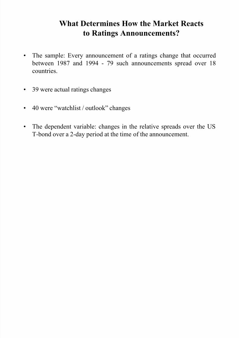
8/13/2019 00000chen- Linear Regression Analysis3
http://slidepdf.com/reader/full/00000chen-linear-regression-analysis3 233/252
• The sample: Every announcement of a ratings change that occurred
between 1987 and 1994 - 79 such announcements spread over 18
countries.
• 39 were actual ratings changes
• 40 were “watchlist / outlook” changes
• The dependent variable: changes in the relative spreads over the US
T-bond over a 2-day period at the time of the announcement.
What Determines How the Market Reacts
to Ratings Announcements? Explanatory variables.

8/13/2019 00000chen- Linear Regression Analysis3
http://slidepdf.com/reader/full/00000chen-linear-regression-analysis3 234/252
0 /1 dummies for
- Whether the announcement was positive
- Whether there was an actual ratings change
- Whether the bond was speculative grade
- Whether there had been another ratings announcement in the previous 60 days.
and
- The change in the spread over the previous 60 days.
- The ratings gap between the announcing and the other agency
What Determines How the Market Reacts
to Ratings Announcements? Results

8/13/2019 00000chen- Linear Regression Analysis3
http://slidepdf.com/reader/full/00000chen-linear-regression-analysis3 235/252
Dependent Variable: Log Relative SpreadIndependent variable Coefficient (t -ratio)
Intercept -0.02(-1.4)
Positive announcements 0.01(0.34)
Ratings changes -0.01(-0.37)
Moody’s announcements 0.02(1.51)
Speculative grade 0.03**
(2.33)Change in relative spreads from day – 60 to day -1 -0.06
(-1.1)
Rating gap 0.03*(1.7)
Other rating announcements from day – 60 to day -1 0.05**(2.15)
Adjusted R2 0.12
Note: * and ** denote significance at the 10% and 5% levels respectively. Source: Cantor and Packer
(1996). Reprinted with permission from Institutional Investor .
Conclusions

8/13/2019 00000chen- Linear Regression Analysis3
http://slidepdf.com/reader/full/00000chen-linear-regression-analysis3 236/252
• 6 factors appear to play a big role in determining sovereign credit
ratings - incomes, GDP growth, inflation, external debt, industrialised
or not, and default history.
• The ratings provide more information on yields than all of the macro
factors put together.
• We cannot determine well what factors influence how the markets will
react to ratings announcements.
Comments on the Paper

8/13/2019 00000chen- Linear Regression Analysis3
http://slidepdf.com/reader/full/00000chen-linear-regression-analysis3 237/252
• Only 49 observations for first set of regressions and 35 for yield
regressions and up to 10 regressors
• No attempt at reparameterisation
• Little attempt at diagnostic checking
• Where did the factors (explanatory variables) come from?

8/13/2019 00000chen- Linear Regression Analysis3
http://slidepdf.com/reader/full/00000chen-linear-regression-analysis3 238/252

8/13/2019 00000chen- Linear Regression Analysis3
http://slidepdf.com/reader/full/00000chen-linear-regression-analysis3 239/252
Example:• Simple Regression Results
Coefficients tandard Erro t Stat F-Value 9.89

8/13/2019 00000chen- Linear Regression Analysis3
http://slidepdf.com/reader/full/00000chen-linear-regression-analysis3 240/252
• Multiple Regression Results
• Check the size and significance level of the
coefficients, the F-value, the R-Square, etc. Youwill see what the “net of “ effects are.
Intercept (b0) 165.0333581 16.50316094 10.000106
Lotsize (b1) 6.931792143 2.203156234 3.1463008
Adjusted R Square 0.108
Standard Error 36.34
Coefficients Standard Error t Stat Intercept 59.32299284 20.20765695 2.935669
Lotsize 3.580936283 1.794731507 1.995249
Rooms 18.25064446 2.681400117 6.806386
F-Value 31.23Adjusted R Square 0.453
Standard Error 28.47
Using The Equation to Make Predictions
• Predict the appraised value at average lot size
(7.24) and average number of rooms (7.12).

8/13/2019 00000chen- Linear Regression Analysis3
http://slidepdf.com/reader/full/00000chen-linear-regression-analysis3 241/252
• What is the total effect from 2000 sf increase in
lot size and 2 additional rooms?
$215,180or 215.18
)18.25(7.12(7.24)3.5859.32. App.Val
in app. value
(3.58)(2000) (18.25)(2)
$43,660
Increse
Coefficient of Multiple Determination, r2 and
Adjusted r2
• Reports the proportion of total variation in Y

8/13/2019 00000chen- Linear Regression Analysis3
http://slidepdf.com/reader/full/00000chen-linear-regression-analysis3 242/252
explained by all X variables taken together (the
model)
• Adjusted r2
• r2 never decreases when a new X variable is added to
the model
– This can be a disadvantage when comparing models
squaresof sumtotal
squaresof sumregression
SST
SSRr 2 k..12.Y
• What is the net effect of adding a new variable? – We lose a degree of freedom when a new X variable is added
– Did the new X variable add enough explanatory power to offset
the loss of one degree of freedom?

8/13/2019 00000chen- Linear Regression Analysis3
http://slidepdf.com/reader/full/00000chen-linear-regression-analysis3 243/252
• Shows the proportion of variation in Y explainedby all X variables adjusted for the number of X
variables used
(where n = sample size, k = number of independent variables)
– Penalize excessive use of unimportant independent
variables
– Smaller than r2
– Useful in comparing among models
1k n
1n
)r 1( 1r
2
k ..12.Y
2
adj
Multiple Regression Assumptions• Assumptions:

8/13/2019 00000chen- Linear Regression Analysis3
http://slidepdf.com/reader/full/00000chen-linear-regression-analysis3 244/252
• The errors are normally distributed• Errors have a constant variance
• The model errors are independent
• Errors (residuals) from the regression model:
ei = (Yi – Yi)
• These residual plots are used in multiple regression:
– Residuals vs. Yi
– Residuals vs. X1i
– Residuals vs. X2i
– Residuals vs. time (if time series data)
Two variable model
Y
bbbˆ

8/13/2019 00000chen- Linear Regression Analysis3
http://slidepdf.com/reader/full/00000chen-linear-regression-analysis3 245/252
X1
X2
22110 X b X bbY Yi
Yi<
x2i
x1i
The best fit equation, Y ,
is found by minimizing the
sum of squared errors, e2
<
Sample
observation
Residual = ei =
(Yi – Yi)<
Are Individual Variables Significant?
• Use t-tests of individual variable slopes

8/13/2019 00000chen- Linear Regression Analysis3
http://slidepdf.com/reader/full/00000chen-linear-regression-analysis3 246/252
• Shows if there is a linear relationship between the
variable Xi and Y; Hypotheses:
• H0: βi = 0 (no linear relationship)
• H1: βi ≠ 0 (linear relationship does exist between Xi and Y)
• Test Statistic:
• Confidence interval for the population slope βi
ib
i1k n
S
0bt
ib1k ni S t b
Is the Overall Model Significant?
• F-Test for Overall Significance of the Model
h f h l l h b ll f h

8/13/2019 00000chen- Linear Regression Analysis3
http://slidepdf.com/reader/full/00000chen-linear-regression-analysis3 247/252
• Shows if there is a linear relationship between all of the X variables considered together and Y
• Use F test statistic; Hypotheses:
H0: β
1 = β
2 = … = β
k = 0 (no linear relationship)
H1: at least one βi ≠ 0 (at least one independentvariable affects Y)
• Test statistic:
1k n
SSE
k
SSR
MSE
MSR F
Testing Portions of the Multiple RegressionModel
f d f l f d d l j
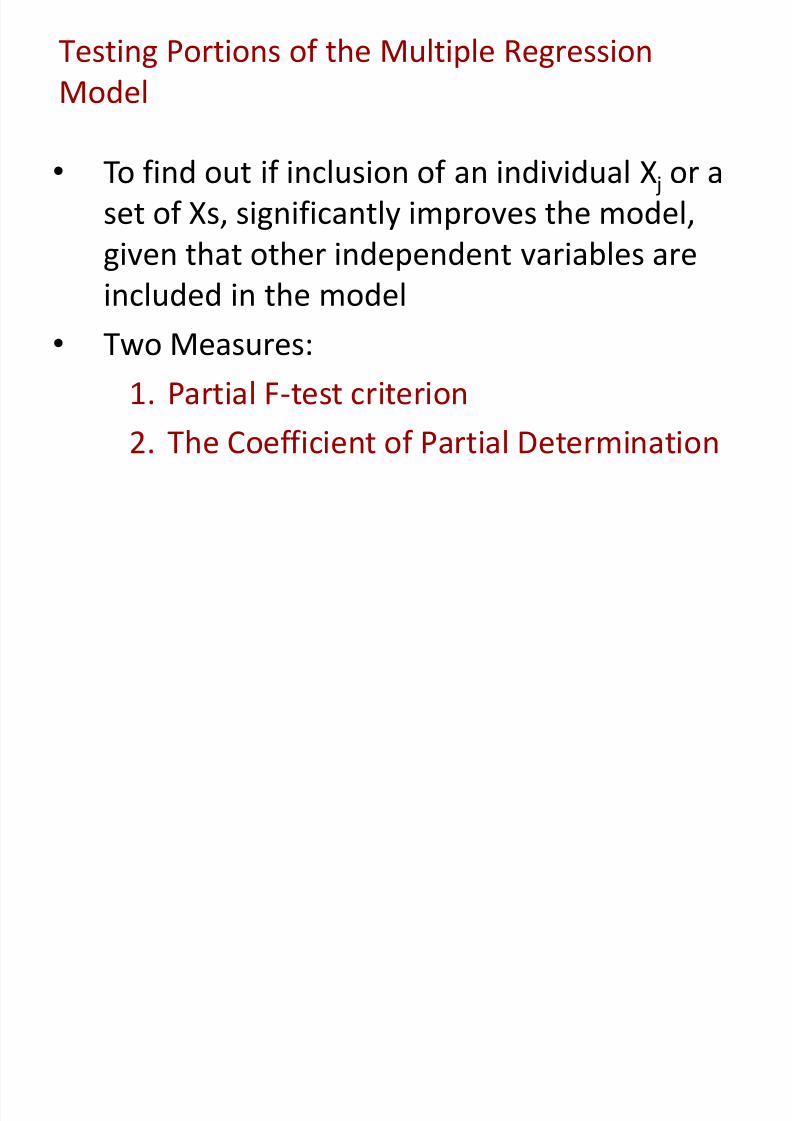
8/13/2019 00000chen- Linear Regression Analysis3
http://slidepdf.com/reader/full/00000chen-linear-regression-analysis3 248/252
• To find out if inclusion of an individual X j or aset of Xs, significantly improves the model,
given that other independent variables are
included in the model• Two Measures:
1. Partial F-test criterion
2. The Coefficient of Partial Determination
Contribution of a Single Independent
Variable X j
SSR(Xj | ll i bl Xj)

8/13/2019 00000chen- Linear Regression Analysis3
http://slidepdf.com/reader/full/00000chen-linear-regression-analysis3 249/252
SSR(X j | all variables except X j)= SSR (all variables) – SSR(all variables except X j)
• Measures the contribution of X j in explaining the total
variation in Y (SST)
• consider here a 3-variable model:SSR(X1 | X2 and X3)
= SSR (all variablesX1-x3) – SSR(X2 and X3)
SSRUR
Model
SSRR
Model
The Partial F-Test Statistic• Consider the hypothesis test:
H0: variable Xj does not significantly improve the model after all

8/13/2019 00000chen- Linear Regression Analysis3
http://slidepdf.com/reader/full/00000chen-linear-regression-analysis3 250/252
0other variables are included
H1: variable Xj significantly improves the model after all other
variables are included
1)-k - /(nSSE MSE
n)restrictioof number )/(df SSR-(SSR F
UR
RUR
Note that the numerator is the contribution of X j to the regression.
If Actual F Statistic is > than the Critical F, then
Conclusion is: Reject H0; adding X1 does improve model
Coefficient of Partial Determination for one or aset of variables
• Measures the proportion of total variation in the dependent
i bl (SST) th t i l i d b X hil t lli f

8/13/2019 00000chen- Linear Regression Analysis3
http://slidepdf.com/reader/full/00000chen-linear-regression-analysis3 251/252
variable (SST) that is explained by X j while controlling for(holding constant) the other explanatory variables
RUR
RUR2
j)except variablesYj.(all
SSRSST SSR-SSRr

8/13/2019 00000chen- Linear Regression Analysis3
http://slidepdf.com/reader/full/00000chen-linear-regression-analysis3 252/252
Too complicated
by hand!
Why & How it works?